On the persistence of output fluctuations in high technology sectors

On The Persistence of Output Fluctuations

In High Technology Sectors

by

Marta Aloi,1 Laurence Lasselle,2,* David McMillan2

Abstract

Fatás (2000) argues that in a cross-section analysis of countries there exists a positive correlation between long-term growth rates and the persistence of output fluctuations. The current paper extends this line of research by examining manufacturing sectors of an economy which can be characterised by two levels of technology; a low level and a high level. Analysis of the data reveals a positive correlation between long-term growth rates and the persistence of output fluctuations in ‘high-tech’ sectors. This empirical analysis is further supported by reformulating the model of Matsuyama (1999b) in a stochastic environment. Within this framework the model is able to capture the two main theories of growth, namely; the Solow model and the Romer model. The stochastic nature of the long run output trend is endogenous and based on technological shocks. Despite the cyclical nature of the shocks we are able to show that output fluctuations are more persistent in ‘high-tech’ sectors.

JEL classification: E32, D43

Keywords: Persistence, Growth, Endogenous Fluctuations, Stochastic Trends

1 _{Department of Economics, University of Nottingham, Nottingham, NG7 2RD.}

2

Department of Economics, University of St. Andrews, St. Andrews, Fife, KY16 9AL, U.K.

1.

Introduction

Explaining the occurrence and duration of business cycles has been a recurrent theme in macrodynamic research. Regardless of the theoretical framework in which the model is set, the existence of output fluctuations is recognised. In a stochastic environment the

explanation for such fluctuations is often connected to real business cycle theory (Kydland and Prescott, 1982). Stochastic fluctuations are the result of exogenous shocks

to the fundamentals of the economy (for example, technology). Whilst in a deterministic framework, endogenous fluctuations may appear once agents’ expectations are specified (Grandmont, 1985). However, a central issue that remains concerns whether these

fluctuations persist over time.

According to real business cycle theory, business cycles, in themselves, do not change the long run output trend of the economy in a stochastic framework. It is thought

that the occurrence of a technological shock causes output fluctuations that are transitory in nature. However, this conclusion has recently been put in question. In particular, Fatás

(2000) finds a positive correlation between the persistence of business cycle fluctuations and the level of growth in a cross-country analysis. This empirical finding is then supported by the use of a stylised endogenous growth model with exogenous cyclical

shocks. The conjecture being that growth dynamics are an important element in the persistence of output fluctuations, which requires further study in other economic

settings.

fluctuations may be correlated at a sectoral level. If industries are characterised by different levels of technology, e.g. ‘high-tech’ and ‘low-tech’, it is likely that these

industries will also experience different levels of growth. Typically, innovation occurs in ‘high-tech’ industries which also show rapid growth, whereas growth in traditional less

innovative manufacturing sectors is usually low. If this is the case, then transitory technology shocks will not exert the same effect across industries, and indeed will be more persistent the higher the level of technology used in production. This in turn implies

that economies characterised by a high proportion of ‘high-tech’ industries may display persistent fluctuations and rapid growth, whereas economies based on ‘low-tech’

traditional manufacturing industries are more likely to show low growth and highly transitory fluctuations. From a macroeconomic point of view we can also explain how a given economy may experience different growth dynamics and cyclical fluctuations over

different periods of time depending on its industrial structure.

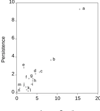
In the analysis presented here empirical evidence on US manufacturing sector

supports our initial intuition. A positive and high correlation can be clearly seen in Figure 1 between the persistence of cyclical fluctuations and the level of growth in ‘high-tech’ sectors. While the persistence of fluctuations is less significant in ‘low-tech’ sectors

characterised by low growth. From a theoretical point of view, this evidence seems to fit with the framework introduced by Matsuyama (1999b) in which growth equilibrium

The remainder of the paper is organised as follows. Section 2 presents the empirical evidence, Section 3 presents the theoretical model, Section 4 is devoted to

discussion of this model, while Section 5 summarises and concludes.

2.

Empirical evidence

Monthly data is taken from the US Governments Federal Reserve - Board of Governors Industrial Production series for the period 1967:1 to 2000:3. The series include output

for: advanced processing; aerospace; chemicals; computers, communications and semiconductors; durable manufacturing; electrical machinery; industrial machinery and

equipment; iron and steel; mining; motor vehicles and parts; non-durable manufacturing; textile mill products; transportation equipment; and utilities. Within this data set sectors such as computers, communications and semiconductors, industrial and electrical

machinery, chemicals and advanced processing can be seen as relatively ‘high-tech’ sectors, compared to ‘lower-tech’ sectors such as iron and steel, mining and textiles, with

the remaining sectors being less obviously classified. All data are presented in logarithms.

Following Fatás (2000) we present, in Figure 1, a plot comparing the degree of

persistence in output, measured against the average annual growth rate in output for each of our series. The measure of persistence used is that of Cochrane (1988), whose variance

ratio measure is given by the following:1

1

) x x ( var

) x x ( var (1/J) = V

1 -t t

J -t t J

where J is the ‘window’ or lag length over which persistence is measured. In the analysis conducted here J is equal to 60, which represents 5 years, and is thus the same time horizon as used in Fatás. The resultant plot is presented in Figure 1, and suggests a

positive correlation between average annual growth rate and persistence of output growth to shocks. Higher growth sectors (the identified ‘high-tech’ sectors of computers,

communications and semiconductors, electrical and industrial machinery and advanced processing) also exhibit a higher degree of persistence, while the ‘low-tech’ sectors (mining, iron and steel, and textiles) which have low growth exhibit low persistence of

output fluctuations.

This graphical analysis is further complemented by a simple cross-section

regression of the following form:

ε α

α0 1 i i

i = + Average Growth +

e Persistenc

where i indexes each industrial sector. The results show a positive and significant relationship between persistence and growth, with the coefficient estimates being -0.4158

(-1.0469) and 0.5687 (8.2667) on α₀ and α₁ respectively (heteroscedasticity robust

standard errors in parentheses). In addition, with the R2 of above regression being 0.8713, this suggests a high explanatory power of average growth rates for output

persistence.

In the following section we present a model that is capable of generating this observed correlation. Growth is driven by investment in physical capital, and uncertainty

3.

The model: a theoretical explanation

3.1.The model under certainty (Matsuyama, 1999b)2

The model contains an infinitively-agent framework with inelastic labour supply. Time is discrete and goes from zero to infinity. There is a final good, taken as numeraire, which is

competitively produced and is either consumed or invested. Let us first highlight that K_t

denotes the capital stock available at the end of period t. It is equal to the amount of the

final good left unconsumed in period t and carried over to period t+1. Therefore, the

capital stock used in period t+1 is denoted by K_t. We assume that there is a positive

amount of capital stock in the first period, i.e. K₀>0.

3.1.1. Preferences

In period t the income of the representative agent takes two forms: the capital income,

t t K

r₋₁ , and the wage income, w_tL. This income allows the agent to consume an amount

t

C of the final good that results from the intertemporal utility function:

( )

t 0

C ln

∑ = ∞

=

t t t

C

U Max

t

β

(where 10< β < is the discount rate) subject to the flow budget constraint:

t t

t Y C

K = − . (1)

The intertemporal solvency condition, which rules out a Ponzi-scheme:

0 lim

1

≥ Π

= ∞ →

t t

r K τ τ

The optimal consumption path is then characterised by the Euler equation:

0 1

1 1 _>

=

+ +

t t

t C

r

C β (2)

and the binding intertemporal solvency condition:

0 lim

lim

1

= =

Π →∞

= ∞

→ _τ

τ τ

τ τ

τ β C

K

r K

t t

.

3.1.2. Production

The final good, Y_t, is competitively produced, and is either consumed or invested. The

part invested is converted into a variety of differentiated intermediate products, and associated with labour (exogenously fixed) according to a Cobb-Douglas technology. The intermediate products are aggregated into a symmetric CES technology. Therefore, the

final goods production function is given by:

( )

σ

( )

σ 1 1

0 1

−

    

   ∫

= Nt t

t A L x z dz

Y

where x_t

( )

z is the intermediate input of variety z∈

[

0,N_t

]

and σ∈

( )

1,∞ is the elasticity

of substitution between each pair of intermediates3 and

[

0,N_t

]

represents the range of

intermediates available at period t.

Define xc as the intermediate input produced in the competitive sector (with no

innovation), and xm the intermediate input produced in the monopolistic innovative

2 _{Sections (3.1.1-3.1.2) largely follow Matsuyama (1999b).}

3

sector. In the sector with no innovation, firms are price takers and there are constant

returns to scale of production. These intermediates are in the range

[

0,N_t−1

]

. They are produced by a units of capital into one unit of an intermediate. The ‘new’ intermediates

are in the range of

[

N_t−1,N_t

]

and may be introduced and sold by innovators in period t. These require F units of capital to innovate and a units of capital per output. There is no barrier to entry. Demands for intermediate inputs come from maximisation of the final

good producers’ profit function, taking into account that all the intermediates enter

symmetrically into the production of the final good, i.e. x_t

( )

z ≡x_tc for z∈

[

0,N_t−1

]

and

( )

m t t z x

x ≡ for z∈

[

N_t−1,N_t

]

. Under these assumptions,

θ σ

σ

≡       − =        

= 1 1 −

m t

c t m t

c t

p p x

x

where θ∈

(

1,e≅2.7183

)

is a parameter related to the monopoly margin of the innovator

(i.e. 1

(

σ−1

)

). Thus, θ =1 when σ is close to one, and θ =e as σ →∞. Which implies

that the demand for each intermediate input reads as:

(

a F

)

x_tc =1 θσ and x_tm =

(

σ−1

)

F a.

By use of these relationships and the economy’s resource constraint on capital in period t,

we have:

(

N N

)

(

ax F

)

x

a N

K_t−1= _{t−1 t}c + _t − _{t−1 t}m+

which implies:

{

1

}

min 1

1 F k_t-1,

a x

a _tc =θσ

   

σ −

= −σ , where

t t t

FN K k

and

(

)

{

1

} ( )

1 1

1 1

1 _{− −}

− = + t − = t

t

t _{Max , k k}

N N

ψ

θ .

Total output is equal to:

( )

( )

(

)

( )

_ 

 _{+ −}

= σ ₋ − σ ₋1 1−1σ

1 1 1

1 m

t t t c

t t

t Aˆ L N x N N x

Y

which can be rewritten as:

( )

{

}

( )

1

1 1 1

− −

−

− = t = t

t

t _{Max A k ,A A k}

K Y

φ

σ _where σ

θσ

1

    ≡

F aL a Aˆ

A .

Before proceeding, let us simplify the notation by assuming a=1, 1L= and F =1

( )

θσ .

Therefore, k_t ≡K_t N_t and A≡Aˆ.

When 1k_t−1< , no innovation can take place. The resource available in the economy is too small relative to the number of products. In this case, we can say that the

economy is in the Solow regime. When k_t−1>1, there is enough resource in the economy to create new products. We can then say that the economy is in the Romer regime. The

critical level of k that separates the two regimes is 1.

3.1.3. Dynamics

The dynamical system governing this economy is derived as follows. First, rewrite the flow budget constraint (1) as:

( ) ( )

t t

t t t

t _k

k k k A N C

− =

− − −

1 1 1 _ψ

φ

1 1 1 1 + + + + = t t t t t t t N C r N N C N β

in addition we know that in equilibrium Y_t =w_tL+r_tK_t−1 and

(

)

t

(

) ( )

t t

t K Y A k

r ₋₁= 1−1σ = 1−1σ φ . Therefore, (2) becomes:

( )

( )

( )

t

(

( )

t

) ( )

t

( )

t t t t t t t k k k A k k A k k k A k k ψ φ φ σ β ψ φ ψ 1 1 1 1

1 1 1

+ − − − − − − = −

which is equivalent to:

( )

( )

(

(

( )

)

) ( )

(

(

) ( )

( ) ( )

)

1

( )

1 1 1 1 1 1 1 − − − + = + − − − t t t t t t t t t t t t k k k A k k A A k k k A k k Ak k ψ ψ φ φ σ β ψ φ σ β ψ φ .

This is a second-order difference equation in k_t, k_t−1 that can be rewritten as a system of two first order difference equations by a simple change of variables (h_t+1=k_t). Let us denote G≡Aβ

(

1−1σ

)

, we then obtain:

(

) ( )

( )

( ) ( )

( ) ( )

    − + = = + + t t t t t t t t t t t h k h k AGh k k k G A k k h ψ ψ φ φ ψ φ 1 1

3.1.4 Steady state analysis4

Steady state values can be easily computed from the Euler equation. A steady state k is

such that k_t =k_t+1. Therefore, we have ψ

( )

k =Gφ

( )

k . In the Solow regime, i.e. k_t <1, then k =Gσ . The economy does not grow. In the Romer regime, i.e. k_t >1, then

4

1 1₊

− =

θ

G

k . In this steady state, new products are introduced and K and N grow at the

same rate, which is the balanced growth path:

( )

1

1 1

1

> = =

=

= ∞

− −

−

G k N

N K

K Y

Y

t t t

t t

t _{ψ .}

3.2. Uncertainty and dynamics

We now introduce uncertainty in the model and assume exogenous transitory technology

shocks. For this purpose a new variable Z_t+1 is introduced into the production function to capture the state of technology at the outset of period t. The production function is now given by:

     

≥ =

≤ =

− −

− −

− −

1 if

1 if

1 1

1 1

1 1

t t

t t

t t

t t

t

k Z

A K

Y

k k

Z K

Y _σ

Following Fatás (2000) we assume that uncertainty originates in Z_t which follows a

stochastic process with the Wold representation:

( )

t t C L

zˆ = ε .

For simplicity we assume that the steady state value of Z_t is 1. C

( )

L is a lag polynomial,

( )

= + + 2 +!

2 1

1 c L c L L

C where all roots are assumed to be less than one to ensure

stationarity of the stochastic process. Stationarity of zˆ allows us to refer to this process

(

X −X

)

X ≈dlogX in the neighborhood of X , the ‘hat’ notation is used to denote log

deviations from the steady state.

Let us now evaluate the FOC of the maximization of the expected utility function, i.e. the Euler equation of the model under uncertainty:

( )

( )

₋ −

( )

₋ = _

( )

−+ ₊

( )

_ − − t t t t t t t t t t t k k k A k r E k k k A k k ψ φ β ψ φ ψ 1 1 1 1 1 1 (3)

Equation (3) together with the flow-budget constraint describes the new equilibrium dynamics of the model. The solution of this system of equations is found by

log-linearisation around the steady state. A few computations (see Appendix B) yields:

1 1

1 + +

− = +

+

+ t t t t t t

t ckˆ akˆ E kˆ dE zˆ

zˆ

b (4)

where

(

)

       ≥ − = − + = − = − = ≤ − = + − = − = − = 1 if 1 1 1 1 if 1 1 1 1 1 1 t-k d , G A c , G A b , G A a k d , G A c , G A b , a θ θ σ β

Let us assume that zˆ_t follows an AR(1) process:

t t t zˆ

zˆ =ρ ₋₁+ε

Equation (4) can be then rewritten as:

(

)

t

(

)

t

t b d zˆ c kˆ

kˆ

a ₋₁+ − ρ = ρ−

t t zˆ c aL b d kˆ     + − − = ρ ρ (5)

We now need to substitute this solution into the log-differentiated production function and the log-differentiated flow-budget constraint (see Appendix C) to find an expression for the deviations of output growth from its steady state value, that is:

(

)

t t

(

(

)

) ( )

t

t L zˆ Lzˆ L C L

y

ˆ = − +ω = − −ω ε

∆ 1 1 1

where

(

)

        ≥       + − −       _{− +}       − = ≤       + − −     ₋       −       + = − − 1 if 1 1 1 if 1 1 1 1 2 1 t t k L c aL b d G A G A k L c aL b d G A G A ρ ρ θ ω ρ ρ σ ω

This expression can be used to evaluate the stochastic properties of output, and is similar

to the expression found by Fatás (2000). Let X ≡ β

(

1−1σ

)

=G A and assume

1

0<ω < .

Proposition

0

> ∂

∂ω A if 0< L< X .

Proof: See Appendix D.

4.

Discussion

Following Fatás (2000), we now turn to the measure of persistence. As highlighted in Section 2 the measure of persistence we have chosen is that proposed by Cochrane

(1988). While, our model generates a unit-root output process as long as ω ≠0. Recall

that V can be written as:

( )

(

ρ

)

(

ω

(

ρ

)(

ω

)

)

ρ ω

− − + −

− =

1 1 2 1

1

2 2

2 2

V

A straightforward computation shows that V is increasing in ω which is increasing in A.

Therefore, ‘high-tech’ sectors will have a higher steady state growth rate and a higher ω.

Since V is increasing in ω, this explains the positive correlation between persistence and long-term growth rates, as shown in Figure 1.

4.2 Analysis

Let us consider a multi-sector economy, whose sectors can be characterised by different

levels of technology. No innovation takes place in the ‘low-tech’ sectors, while innovation takes place in the ‘high-tech’ sectors. Assume that the whole economy is

affected by an exogenous transitory technological shock. Our findings show that in sectors with low technology, the correlation is empirically very small and, if we associate the ‘low-tech’ sectors to the Solow Regime, should be theoretically nil. ‘High-tech’

sectors show persistent fluctuations because of the positive correlation between persistence and rates of growth. In our model presented here, the higher is the rate of

growth, the higher is the prospect of fluctuations and the higher is their persistence. We can further point out that in a stochastic setting, the model exhibits fluctuations for the same parameter values as in the deterministic setting (see Appendix

ways. First, the business cycles in these ‘high-tech’ sectors overbalance what is happening in the ‘low-tech’ sectors. Second, as shown by Matsuyama (1999a, 1999b)

there exists a link between the two regimes. This model explains how in a deterministic setting the economy can oscillate between two phases of growth. Assume that the

economy is initially at the stationary balanced growth path (i.e. the Romer regime). If the steady state loses its stability endogenous fluctuations can appear such that it becomes possible for the economy to cycle between phases of high investment-low innovation and

low-investment-high innovation. Recall from Section 3 that when more resource are available in the economy, innovation takes place, new goods are introduced and

innovators enjoy their monopoly rents. The economy can then steadily grow at the rate defined in the Romer regime. This, however, is just a temporary phenomenon since there are no barriers to entry. The economy will then return to a phase of no innovation where

it grows solely by capital accumulation, and so forth. This analysis allows us to explain the rise of the total output in the overall economy thanks to a switch between the sectors,

one sector driving the other sector. Periods of high investment are followed by periods of high innovation. Both regimes are then alternatively leading to make the economy grow faster. But recall that in this model the ‘high-tech’ sectors are the more responsive to

5.

Concluding comments

Recent research has suggested that a positive correlation may exist between the persistence of output fluctuations and long-run growth rates of output for industrialised economies, which can be explained through a stylised endogenous growth model. This

paper seeks to extend that research by examining sectoral data for a single country. The empirical evidence again supports a positive correlation between the persistence of output

fluctuations and long-run growth rates for individual sectors. Further, we extend the theoretical framework by reformulating the model of Matsuyama (1999b) in a stochastic framework. Considering a multi-sector economy this model captures the different engines

of growth, and allows us to study the effects of transitory technological shocks on the dynamics of growth. We are able to show that in a stochastic framework cyclical

fluctuations experienced by ‘high-tech’ industries have a positive impact upon growth, while similar fluctuations experienced by ‘low-tech’ sectors have little or no effects on growth. Thus, the model explains why economies experience different growth dynamics

and cyclical fluctuations depending on their industrial structure.

The model presented here, we believe, provides an interesting first step for future research. A natural extension of this work would be to evaluate the impact of a subsidy to these ‘high-tech’ industries when the overall economy is performing poorly. Since these

sectors appear to be more responsive to fluctuations, it would be of interest to study if the implementation of such a policy improves the state of the overall economy and its

welfare, the consequences of implementing of a redistributive tax on the 'high-tech' industries to the 'low-tech' industries.

References

Fatás, A. (2000). "Endogenous growth and stochastic trends," Journal of Monetary Economics 45, 107-128.

Grandmont, J.M. (1985). "On endogenous competitive business cycles," Econometrica

53, 995-1046.

Kydland, F.E. and Prescott, E.C. (1982). "Time to build and aggregate fluctuations,"

Econometrica 50, 1345-1370.

Matsuyama, K. (1999a). "Growing through cycles," Econometrica 67, 335-347.

Matsuyama, K. (1999b). "Growing through cycles in an infinitely-lived agent economy,"

Northwestern University, DP No. 1280.

Appendix

The appendices below describe the techniques used in this paper. Appendix A contains

the computation of the Hessian Matrix of the system in the deterministic case. Appendix B contains the log-linearisation of the Euler equation that helps us to find the solution of

the model. Appendix C resumes the different steps to find the expression for the deviations of output growth from its steady state value. Appendix D explains the different

Appendix A: Stability properties of the steady state in the deterministic case

In the Solow regime the Hessian matrix evaluated at the steady state is equal to:

 

  





 _{− + −}

0 1

1 1

1

β

σ G

A

The trace is equal to 1− σ1 +A G. The determinant is equal to 1 β . Recall that the

characteristic polynomial is: p(λ)=λ2 −trace

( )

λ +determinant. After straightforward

computations, we obtain: λ

( )

1 >0 and λ

( )

−1 <0. Therefore, the steady is a saddle.

In the Romer regime the Hessian matrix evaluated at the steady state is equal to:

(

)

    

 

 − + −

0 1

1 1

2

G A G

A θ

θ

The trace is equal to

(

1−θ +A

)

Gand the determinant is A

(

θ −1

)

G2. One eigenvalue of

the characteristic polynomial is always greater than 1. The other eigenvalue is always

negative, but can be less or greater than -1. Therefore,

If 1− <−1

G

θ

, the other eigenvalue is less than –1. The steady state is a source.

If −1<1− <0

G

θ

, the other eigenvalue is greater than –1. The steady state is a saddle.

Appendix B

and obtain a linear difference equation in the logs of k and the exogenous technological

shock Z. Second, we find a solution of this expression, rewriting equation (3) as:

(

)

₍

₎

_      = + + + − 1 1 1 1 t t t t t t t t k , k , Z g r E k , k , Z f β where

(

)

_{( )}

( )

_{( )}

1 1 1 1 1 − − − − − ≡ ₋ t t t t t t t t t k k k AZ k k k , k , Z f ψ φ ψ and

(

Zt ,kt,kt

)

ktAZt

( )

kt kt

( )

kt

g _{+1 +1} ≡ ₊₁φ − ₊₁ψ .

Assume that the random variable on the right-hand side of (3) is log-normally distributed

with a conditional variance that is constant over time. By use of the properties of log-normal random variables, (3) can then be written as:

(

)

( )

(

(

)

)

₍

[ ]

₎

                    + − = + + + + + + − 1 1 1 1 1 1

1 Var log

2 1 log log exp t t t t t t t t t t t t k , k , Z g r k , k , Z g r E k , k , Z f β

taking logs of both sides yields:

(

)

₍

[ ]

₎

( )

1

(

(

1 1

)

)

1

1 1

1 Var log log log

2 1 log

log _{+ + +}

+ + + − + −      +

= _{t t t t t t}

t t t t t t

t E r E g Z ,k ,k

k , k , Z g r k , k , Z f β

Since

[ ]

(

)

o

t t t t k , k , Z g r χ ≡       + + + 1 1 1 log Var 2 1

is a constant and the steady state interest rate

equals 1 β this equation can be expressed in terms of deviations from the steady state as:

(

Zt,kt ,kt

)

Et

( )

rt Et

(

g

(

Zt ,kt,kt

)

)

o

Since we are interested in the system’s dynamic response to shocks, we omit the constant

0

χ and we totally differentiate the approximate Euler equation around the steady states

(recall that Z =1):

( )

( )

( ) ( )

(

)

( ) ( )

( )

(

( ) ( )

( ) ( )

)

( )

1

1 − − − ₋ + ₋ − ′ + ₋ − ′ ′ t t t t kˆ k k A k k k k k A kˆ k k A k zˆ k k A k k k A kˆ k k k ψ φ ψ φ φ ψ φ ψ ψ φ φ ψ

( )

( ) ( )

(

)

( )

( ) ( )

(

( ) ( )

( ) ( )

)

( )

(

)

( )

(

)

( )

(

)

(

(

(

)

)

( )

( )

)

t

t t t t t t t t t t t t t t t t t t t t t kˆ k Z AE k Z AE k zˆ E k Z AE k A kˆ k k Z AE k k k k k Z AE kˆ E k k Z AE k zˆ E k k Z AE k A φ σ φ σ φ σ φ σ ψ φ ψ φ φ ψ φ ψ ψ φ φ 1 1 1 1 1 1 1 1 1 1 1 1 1 1 1 1 1 1 + + + + + + + + + + − ′ − + − − + − ′ − + ′ − − + − − =

By substituting the value of the different functions at the steady state values into this

latter expression we obtain:

1 1

1 ˆ ˆ

ˆ 1 ˆ 1

1

ˆ  − ₋ =− ₊ + ₊

     _{− +} +

− t kt kt Etzt Etkt

G A z G A β

σ if 1kt−1≤

(

)

1 1 1 2 1 1 + + − =− +     − +       + − +

− t t kˆt Etzˆt Etkˆt

G A kˆ G A zˆ G

A θ θ

if k_t−1≥1

Appendix C

Here we derive an expression that describes the deviations of output growth from its steady state value. This computation is performed in two steps. First, we log-linearise the

production function around its steady states values. Second, we approximate the budget flow constraint equation around the steady states values in order to evaluate the

The production function is linear in logs and therefore needs no approximation.

( )

1

1 −

−

= _{t t t}

t AK Z k

Y φ with K_t−1=k_t−1N_t−1

which is equivalent to

( )

t

_{( )}

( )

t t t zˆ k k k kˆ k kˆ y ˆ +     ′ + − + = _{− −} φ φ ψ 1 1 1 ⇔

(

)

   ≥ − + + = ≤ + − = − − − − 1 if 1 1 if 1 1 1 1 1 1 t t t t t t t t k G zˆ kˆ y ˆ k zˆ kˆ y ˆ σ

To log-linearise the budget-flow constraint around the steady states we first use the

production function to substitute for Yand then we totally differentiate the result:

( )

( )

( ) ( ) ( ) ( )

_{[ ]}

_{( )}

₂ 1

(

1

)

1 − −  − −      −         _{′ − ′} + =

∆ _{t t t} cˆ_t nˆ_t kˆ_t

k N C kˆ k k k k k k A zˆ k k A kˆ ψ ψ φ ψ φ ψ φ ⇔

(

)

      ≥       _{− +}       − = ∆ ≤     ₋       −       + = ∆ − − − − 1 if 1 1 1 if 1 1 1 1 1 2 1 1 t t t t t t t t k kˆ G A zˆ G A kˆ k kˆ G A zˆ G A kˆ θ σ

The expression of the deviation of the output around the steady states values is then easy

to compute. We just need first to replace kˆ_t−1 by expression (5) into ∆kˆ_t and then implement ∆kˆ_t−1 into ∆ˆy_t.

Appendix D

(

)

      ≥       + − −       _{− +}       − = ≤       + − −       ₋       −       + = − − 1 if 1 1 1 if 1 1 1 1 2 1 t t k L c aL b d G A G A k L c aL b d G A G A ρ ρ θ ω ρ ρ σ ω

We do not study the case of the Solow regime since ∂ω ∂A=0. Turning to the analysis

of the Romer regime, computations yield to the two following remarks:

Remark 1: if X AX

(

X

)

<L

− − −

1 1

θ then 0 − + <1 − < aL c b d ρ ρ

Remark 2: if

(

)

(

(

X

)(

L

)

)

L X X A L L + − + < − < + 2 2 1 1 1 1 4 1 θ

then 0<ω <1.

Proof of the proposition:ω is increasing in A.

(

)

(

)

(

(

)

(

)

)

(

)

(

)

_              + − − − −       + −       −     + − −    _{− − + +} − = ∂ ∂ 2 2 2 1 1 1 1 1 1 1 c aL b d L A G G G A c aL b d G G G L A ρ ρ θ θ ρ ρ θ ω

The first term of this expression into brackets is always negative since Remark 1, θ >1,

1

>

G , and L>0. The last expression into brackets is always positive if G A>L.

Therefore the whole expression is always positive.

Q.E.D.

[image:23.612.138.487.120.507.2]

Figure 1:

Persistence and average annual growth rate

0

2

4

6

8

10

0

5

10

15

20

Average Growth

Persistence

a

b

c

d

e

f g

h

i

j

k

l

m

n

Source: US Governments Federal Reserve, Board of Governors Industrial Production series; 1967:1 to 2000:3

Legenda:

a: computers, communications and semiconductors h:durable manufacturing b: electrical machinery i: utilities

c: industrial machinery and equipment j: textile mill products

d: chemicals k: transportation equipment

e: aerospace l: motor vehicles and parts