Fault detection and diagnostics of a three phase separator

*Corresponding author. Tel +447770149747

E-mail addresses: [email protected], [email protected], [email protected],

[email protected]

Fault detection and diagnostics of a three-phase separator

Marius Vileiniskis*, Rasa Remenyte-Prescott, Dovile Rama and John Andrews

Centre for Risk and Reliability Engineering, University of Nottingham, NG7 2RD, Nottingham, United Kingdom

Abstract

A high demand of oil products on daily basis requires oil processing plants to work with maximum efficiency. Oil, water and gas separation in a three-phase separator is one of the first operations that are performed after crude oil is extracted from an oil well. Failure of the components of the separator introduces the potential hazard of flammable materials being released into the environment. This can escalate to a fire or explosion. Such failures can also cause downtime for the oil processing plant since the separation process is essential to oil production. Fault detection and diagnostics techniques used in the oil and gas industry are typically threshold based alarm techniques. Observing the sensor readings solely allows only a late detection of faults on the separator which is a big deficiency of such a technique, since it causes the oil and gas processing plants to shut down.

A fault detection and diagnostics methodology for three-phase separators based on Bayesian Belief Networks (BBN) is presented in this paper. The BBN models the propagation of oil, water and gas through the different sections of the separator and the interactions between component failure modes and process variables, such as level or flow monitored by sensors installed on the separator. The paper will report on the results of the study, when the BBNs are used to detect single and multiple failures, using sensor readings from a simulation model. The results indicated that the fault detection and diagnostics model was able to detect inconsistencies in sensor readings and link them to corresponding failure modes when single or multiple failures were present in the separator.

Keywords

Three-phase separator, fault detection, fault diagnostics, Bayesian Belief Networks, BBN

1 Introduction

Three-phase separators (TPS) are one of the key components of offshore processing facilities. A failure in the TPS can cause the whole oil processing plant to be stopped. Thus, a timely detection of failing components in the TPS is necessary.

Faults in the TPS and other processing units in the oil and gas industry are commonly detected by using either thresholds of the process variables2 (e.g. oil level, water level and etc.), statistical analysis of the process variables3-6 or precise mathematical models7-10 simulating the operation of the TPS and then comparing its outputs with the readings obtained from the actual separator. The first approach usually detects failures when their effect is already critical and prevention of the separator shut down is unavoidable. Moreover, observing the readings from individual sensors and comparing them to threshold values might hide certain failure modes (level transmitters stuck on the last reading) unless comparison between several sensors is not performed. The second approach needs historical data of the process variables under fault free and faulty operation, which might not always be available in practice, especially for the hazardous failure modes. Finally, the detailed mathematical model approach needs a very good understanding of the process conditions and usually requires extensive modifications if operating conditions change.

A novel fault detection and diagnostic methodology for TPS is proposed in this study. It can give an early warning of a failure in the system and has an ability to be easily adapted for the specific system. The methodology was built using the Bayesian Belief Network (BBN) technique. Such an approach was chosen due to several reasons, including the graphical representation of the modelled system, inclusion of expert knowledge about failure modes of the system, ability to model uncertainties in a probabilistic way, ability to build the model in a structured and modular way and update the prior knowledge about occurrence of certain failure modes without altering the structure of the model.

2 Three-phase separator

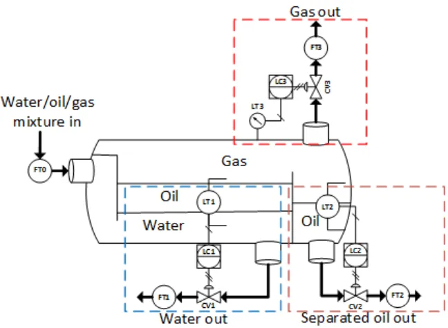
Figure 1. Horizontal three-phase separator schematic of configuration with weir A schematic diagram of a typical horizontal three-phase gravity separator with a weir can be seen in Figure 1. The whole vessel can be roughly divided into three sections:

1. The gravity settling section (or the liquid separation section), where the separation of water and oil takes place (the section to the left of the weir). 2. The separated oil section, where the separated oil flows from the liquid

separation section (the section to the right of the weir).

3. The remaining space of the vessel is left for the gas phase (separated gas section).

The main components to monitor and control the horizontal three-phase separator given in Figure 1 are summarised in Table 1.

Table 1. Components to monitor and control three-phase separator11 Name Component Purpose

FT0 Flow rate transmitter

Measures the multiphase flow (water, oil and gas individually) coming to the separator from the upstream equipment. Provides the information to predict the water, oil and gas level changes in the separator.

LT1 Level transmitter

Measures the levels of water and oil in the gravity settling section. Provides the information to control the water-oil interface level for the safe and efficient use of the separator.

Name Component Purpose

level transmitter.

CV1 Control valve Provides a way to control the water-oil interface level in the gravity settling section by opening/closing when the corresponding command is received from the controller LC1. FT1 Flow rate

transmitter

Measures the flow of the liquid allowed by the opening of the control valve CV1 to monitor the outflowing water from the separator.

LT2 Level transmitter

Measures the level of oil in the separated oil section. Provides the information to control the oil level for the safe and efficient use of the separator.

LC2 PI controller Provides a control command to keep the control valve CV2 at the necessary opening so that the separated oil is maintained at the desired level. Receives the information from the LT2 level transmitter.

CV2 Control valve Provides a way to control the oil level in the separated oil section by opening/closing when the corresponding command is received from the controller LC2.

FT2 Flow rate transmitter

Measures the flow of the liquid allowed by the opening of the control valve CV2 to monitor the outflowing separated oil from the separator.

LT3 Pressure transmitter

Measures the pressure in the separator. Provides the information to control the pressure inside the vessel for the safe and efficient use of the separator.

LC3 PI controller Provides a control command to keep the control valve CV3 at the necessary opening so that the pressure is maintained at the desired level. Receives the information from the LT3 level transmitter.

CV3 Control valve Provides a way to control the pressure inside the separator by opening/closing when the corresponding command is received from the controller LC3.

FT3 Flow rate transmitter

Measures the flow of the gas allowed by the opening of the control valve CV3 to monitor the outflowing gas from the separator.

2.1 Simulation model of a three-phase separator

used in practice, since building a test system can be costly. Moreover, testing using such a system usually takes more time, since all the effects of failures have to be removed from the system before another failure can be induced in the system. It might even be unsafe to induce certain failure modes, which might lead to the damage of the system.

The second option – system models – are favoured, since they can capture the main operating conditions of real systems and are cheap to implement. Furthermore, the data from the models is easily obtainable and even hazardous failure modes can be easily tested. The cost of developing models, the time taken to get the data and the ease of modelling different failures are the most important factors making the system models a preferred option for testing and validating fault detection and diagnostic techniques. The latter approach was also used in the study performed.

Software with a graphical user interface for modelling the operation of a TPS under both normal operating conditions and those affected by faults was written in C++. A simplified model of a TPS was considered. If necessary, the complexity of the simulation model can be increased by modifying the model assumptions. The assumptions used for the TPS modelling are as follows:

1) The separation process is assumed to be perfect. All of the incoming mixture is completely separated into three different phases, i.e. water, oil and gas, and the separation occurs instantly.

2) The layers of the different phases are formed on top of each other and do not mix, just separate.

3) There are no leaks in the separator.

4) The volume of internal components (e.g. inlet diverter, weir) is not considered.

5) The maximum inflow is twice as high as the average inflow. Control valves are designed to allow the same maximum outflow rates as those of the maximum inflows, when the valves are fully open. When outlet valves are half opened, an amount corresponding to an average inflow is released from the vessel.

6) The precision of level transmitters is 1 cm, the precision of the flow rate transmitters is 0.001 m3 (1 litre) and the precision of the pressure transmitter is 1 kPa.

7) Control valves can be opened with a 5% precision ranging from being fully closed (opened 0%) to fully opened (opened 100%).

8) A control command sent from the controller to a control valve is recalculated every 5 seconds, while levels of water, oil and gas are monitored every second.

9) There is no dead time between time points when the level of each phase is measured and sent from the transmitter to the controller; and then the control command is sent from the controller to the control valve.

10) Selected PI control parameters 𝐶𝑂𝑏 (controller bias value), 𝐾𝐶 (controller

gain) and 𝑇𝑖 (integral time) are such that they do not cause a disruption to

the operation of the TPS when all of the control components are working. 11) Physical design parameters of the separator (e.g. weir height, separator

set point, oil level set point), given in Table 3 are assumed to be chosen appropriately.

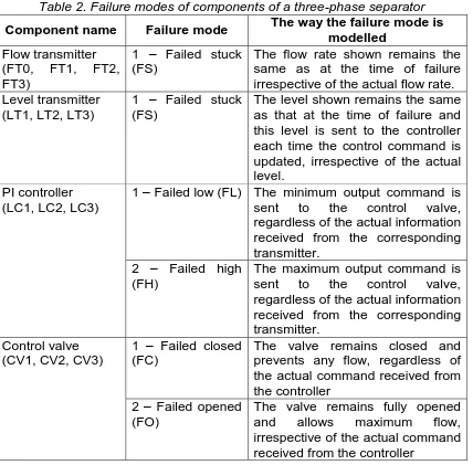
12) Selected failure modes given in Table 2 are only considered for the simulation model.

Table 2. Failure modes of components of a three-phase separator

Component name Failure mode The way the failure mode is modelled

Flow transmitter (FT0, FT1, FT2, FT3)

1 – Failed stuck (FS)

The flow rate shown remains the same as at the time of failure irrespective of the actual flow rate. Level transmitter

(LT1, LT2, LT3)

1 – Failed stuck (FS)

The level shown remains the same as that at the time of failure and this level is sent to the controller each time the control command is updated, irrespective of the actual level.

PI controller (LC1, LC2, LC3)

1 – Failed low (FL) The minimum output command is sent to the control valve, regardless of the actual information received from the corresponding transmitter.

2 – Failed high (FH)

The maximum output command is sent to the control valve, regardless of the actual information received from the corresponding transmitter.

Control valve (CV1, CV2, CV3)

1 – Failed closed (FC)

The valve remains closed and prevents any flow, regardless of the actual command received from the controller

2 – Failed opened (FO)

The valve remains fully opened and allows maximum flow, irrespective of the actual command received from the controller

13) Discrete 1 second time steps are used to model the operation of the TPS. Table 3. Parameters of the three-phase separator model

Parameter Value

Separator radius 2 m

Gravity settling section length 7 m Separated oil section length 3 m

Weir height 2 m

Water-oil interface set point 1 m

Oil level set point 1 m

Pressure set point 500 kPa

Maximum flow through valve CV3 0.15 m3/s

Initial water level 1 m

Initial oil level 1 m

Initial pressure level 500 kPa

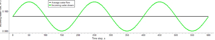
The inflows of oil, gas and water are modelled as oscillating flows with a sine function. The minimum and maximum values of flow, 𝐿𝐵 and 𝑈𝐵 respectively, have to be specified together with a number of full sine waves, 𝑁𝑤𝑎𝑣𝑒𝑠, throughout the

simulation duration, 𝑁𝑠𝑖𝑚. Then the flow can be simulated with a given equation:

𝑓𝑙𝑜𝑤(𝑡) =1

2(sin(𝑥) + 1)(𝑈𝐵 − 𝐿𝐵) + 𝐿𝐵, 2.1

where 𝑓𝑙𝑜𝑤(𝑡) is the simulated flow at time 𝑡 and 𝑥 is defined as follows:

𝑥 =2 ∙ 𝑁𝑤𝑎𝑣𝑒𝑠

𝑁𝑠𝑖𝑚 ∙ 𝑡 ∙ 𝜋, 2.2

where 𝑁_{𝑤𝑎𝑣𝑒𝑠} is the number of full sine waves occurring during the simulation.

Using equations 2.1 and 2.2, the simulated flow is ensured to have a selected number, 𝑁𝑤𝑎𝑣𝑒𝑠, of full sine waves throughout the simulation duration 𝑁𝑠𝑖𝑚. The flow

values range from 𝐿𝐵 to 𝑈𝐵. An example of such flow is given in Figure 2, where

𝑁_{𝑤𝑎𝑣𝑒𝑠}= 3, 𝑁_𝑠𝑖𝑚= 600, 𝐿𝐵 = 0 𝑚3/𝑠 and 𝑈𝐵 = 0.15 𝑚3/𝑠.

Figure 2. Oscillating water inflow as modelled with a TPS simulation model Flows of liquid and gas in the separator are modelled at discrete time steps of 1 second. Even though the movement of materials in the vessel happens simultaneously, it is modelled through discrete changes in their levels in the following order:

1. With the incoming fluid, the levels of liquids and the volume of gas in the gravity settling section are increased accordingly, i.e. the level of water gravity settling section, the level of oil in the gravity settling section and the volume of gas in the separator.

2. The water is the first to leave the separator through valve CV1 and the water level and the total liquid level in the gravity settling section are adjusted accordingly.

4. The oil leaves the separator through valve CV2 and the oil level in the separated oil section is adjusted accordingly.

5. The volume of gas in the separator is calculated.

6. The gas leaves the separator through valve CV3 and the pressure is adjusted accordingly.

This process is repeated at each time step of the simulation.

3 Proposed methodology

3.1 Problem definition and proposed approach

The problem, considered in this study, is to perform fault detection and diagnostics of the components of the TPS given the sensor readings about the undergoing processes in the separator. The idea of the methodology proposed for fault detection and diagnostics is to split the operation period of the TPS into time intervals and then compare sensor readings recorded during several successive time intervals (called time slices in this study) with the expected ones. Irregularities in the readings are considered as a sign of failure of one or more of the TPS components.

A probabilistic model which utilises a Bayesian Belief Network (BBN) is developed in a modular way to replicate the way that water, oil and gas propagate through each section before they leave the separator. This model is used to predict the most likely outcomes of the sensor readings. Modelling the TPS in such a way can overcome the limitations of using threshold values on the process variables, which ignores the interactions between them. Since the three sections of the separator are highly dependent on one another, a failure in one section will usually have a noticeable impact on the other sections. This can be detected if the measuring equipment has not failed in the remaining sections.

Actual sensor readings and several combinations of sensor readings (addition or subtraction of values) from the TPS are then used as input data into a three-phase separator BBN model to identify the readings that do not correspond to the predicted sensor readings from a fault-free system. Effects of the component failures on the sensor readings are modelled in the BBN and given the irregular sensor readings, the probabilities of the failures of components are updated. The probabilities that breach a small threshold value indicate that a certain component failure has occurred in the TPS. The next sections give a brief overview of the BBN technique and the BBNs that were developed for the fault detection and diagnostics of the TPS. 3.2 Bayesian Belief Networks

 A set of variablesand a set of directed edges between variables.

 Each variable has a finite set of mutually exclusive states.

 The variables together with the directed edges form an acyclic directed graph (abbreviated DAG). A directed graph is acyclic if there is no directed path

𝐴₁ → ⋯ → 𝐴_𝑛 so that 𝐴1 = 𝐴𝑛.

 A conditional probability table (CPT) 𝑃(𝐴|𝐵1, … , 𝐵𝑛) is attached to each

variable 𝐴 with parents 𝐵1, … , 𝐵𝑛. If 𝐴 has no parents, then the table reduces

to the unconditional probability table 𝑃(𝐴).

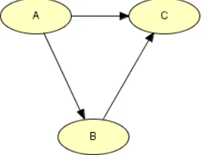
A BBN lends itself to a graphical representation. An example BBN is given in Figure 3.

Figure 3. Example of a BBN

The BBN variables are represented as nodes 𝐴, 𝐵 and 𝐶, which are connected with the directed edges. The direction of an edge identifies the causal relationship enabling the parent and child nodes to be identified from the graphical representation of the BBN. For example, 𝐵 and 𝐶 are child nodes of 𝐴, while 𝐴 is the parent node of

𝐵 and 𝐶. Moreover, 𝐵 is the parent node of 𝐶, thus 𝐶 has two parent nodes. To define the BBN completely, an unconditional probability table 𝑃(𝐴) and conditional probability tables 𝑃(𝐵|𝐴) and 𝑃(𝐶|𝐵, 𝐴) have to be specified. BBNs are usually built using expert knowledge.

The conditional probability of variable A given variable B, P(A|B), can be expressed as:

𝑃(𝐴|𝐵) =𝑃(𝐵|𝐴)𝑃(𝐴)

𝑃(𝐵) =

𝑃(𝐵, 𝐴)

∑ 𝑃(𝐵, 𝐴)_𝐴 , 3.1

In order to show how the information is propagated in the BBN a calculus example is considered for the BBN given in Figure 3.

Table 4. Unconditional probability table for variable A

A a1 0.25

a2 0.75

Table 5. CPT for variable B, P(B|A) A a1 a2

B b1 0.8 0.1

Table 6. CPT for variable C, P(C|A,B)

A a1 a2

B b1 b2 b1 b2

C c1 0.9 0.6 0.4 0

c2 0.1 0.4 0.6 1

The three probability tables given above define the causal relationships between variables A, B and C in this example BBN.

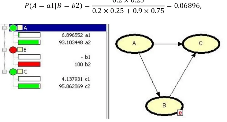
Say, we know that the variable B is in the state ‘b2’, then, given this knowledge, we can update the probability of variable A being in the state ‘a1’, using equation 3.1 in the following way:

𝑃(𝐴 = 𝑎1|𝐵 = 𝑏2) =𝑃(𝐵 = 𝑏2|𝐴 = 𝑎1)𝑃(𝐴 = 𝑎1)

𝑃(𝐵 = 𝑏2) =

= 𝑃(𝐵 = 𝑏2|𝐴 = 𝑎1)𝑃(𝐴 = 𝑎1)

𝑃(𝐵 = 𝑏2|𝐴 = 𝑎1)𝑃(𝐴 = 𝑎1) + 𝑃(𝐵 = 𝑏2|𝐴 = 𝑎2)𝑃(𝐴 = 𝑎2),

3.2

We get the conditional probabilities 𝑃(𝐵 = 𝑏2|𝐴 = 𝑎1), 𝑃(𝐵 = 𝑏2|𝐴 = 𝑎2) from Table 5 and probabilities 𝑃(𝐴 = 𝑎1), 𝑃(𝐴 = 𝑎2) from Table 4 and insert them into the equation 3.2:

𝑃(𝐴 = 𝑎1|𝐵 = 𝑏2) = 0.2 × 0.25

0.2 × 0.25 + 0.9 × 0.75= 0.06896, 3.3

Figure 4. Evidence B=b2 inserted in the BBN 3.3 Fusion of sensor readings

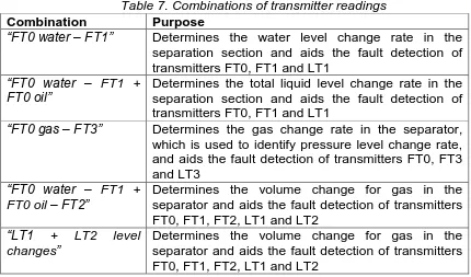
and failure of one of the transmitters can be detected. Combinations of the transmitter readings (addition or subtraction of values) considered in this study are listed in Table 7.

Table 7. Combinations of transmitter readings Combination Purpose

“FT0 water – FT1” Determines the water level change rate in the separation section and aids the fault detection of transmitters FT0, FT1 and LT1

“FT0 water – FT1 + FT0 oil”

Determines the total liquid level change rate in the separation section and aids the fault detection of transmitters FT0, FT1 and LT1

“FT0 gas – FT3” Determines the gas change rate in the separator, which is used to identify pressure level change rate, and aids the fault detection of transmitters FT0, FT3 and LT3

“FT0 water – FT1 +

FT0 oil – FT2” Determines the volume change for gas in the separator and aids the fault detection of transmitters FT0, FT1, FT2, LT1 and LT2

“LT1 + LT2 level

changes” Determines the volume change for gas in the separator and aids the fault detection of transmitters FT0, FT1, FT2, LT1 and LT2

The use of the listed combinations of transmitter readings improves the accuracy of fault detection. For example, if “LT1 + LT2 level changes” and “FT0 water – FT1 + FT0 oil – FT2” readings differ, it indicates that one of the components FT0, FT1, FT2, LT1 or LT2 might have failed.

In the next subsections, the BBNs created for control loops and individual sections are introduced together with a BBN that merges the section BBNs into a BBN for the whole TPS and then the final BBN that was used for fault detection and diagnostics of TPS is presented.

3.4 BBN for a control loop

The main idea behind the proposed methodology is to create a fault detection and diagnostics BBN in a modular way, so that when certain physical characteristics of the TPS change it would be easy to adjust the BBN without redeveloping the whole structure of the BBN. When BBNs are built in this way (using BBNs as a part of another BBN), they are referred to as Object Oriented Bayesian Networks (OOBN)14. The TPS was divided into three sections, each of which contains a control loop (e.g. water-oil interface level control loop in the separation section). A generic BBN built for the control loop, is given in Figure 5. The BBN propagates the information flow in an analogous way to the physical system. For example, sensor LT reads the information about the level of the liquid or gas (“Level transmitter LTi information on

what CVi openness has to be” node) and depending on the condition of the sensor

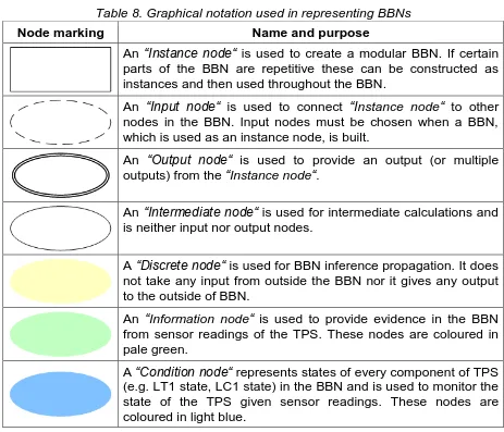
paper. The light blue nodes represent the states of every component in the BBN and will be referred to as “Condition nodes”. The graphical notation used in the BBNs is summarised in Table 8.

Table 8. Graphical notation used in representing BBNs

Node marking Name and purpose

An “Instance node“ is used to create a modular BBN. If certain parts of the BBN are repetitive these can be constructed as instances and then used throughout the BBN.

An “Input node“ is used to connect “Instance node“ to other nodes in the BBN. Input nodes must be chosen when a BBN, which is used as an instance node, is built.

An “Output node“ is used to provide an output (or multiple outputs) from the “Instance node“.

An “Intermediate node“ is used for intermediate calculations and is neither input nor output nodes.

A “Discrete node“ is used for BBN inference propagation. It does not take any input from outside the BBN nor it gives any output to the outside of BBN.

An “Information node“ is used to provide evidence in the BBN from sensor readings of the TPS. These nodes are coloured in pale green.

A “Condition node“ represents states of every component of TPS (e.g. LT1 state, LC1 state) in the BBN and is used to monitor the state of the TPS given sensor readings. These nodes are coloured in light blue.

Note that, the nodes that are not “Condition nodes” are expressed through relative openness of a corresponding valve (for example the state “40 < CV <60” of the node

“Level transmitter LTi information on what CVi openness has to be” indicates a

necessary relative openness of CVi (it has to be opened between 40% and 60% of

Figure 5. BBN “FTi given level LTi” for a control loop

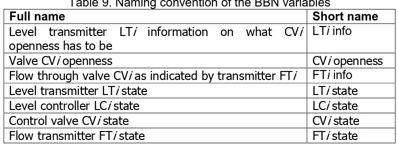
Note that shorter names for the variables used in this BBN will be used in the following sections, when the BBN is used as an instance of other BBNs. The shorter names will be as given in Table 9, where i will correspond to a particular component, for example “LT1 info”.

Table 9. Naming convention of the BBN variables

Full name Short name

Level transmitter LTi information on what CVi openness has to be

LTi info

Valve CVi openness CVi openness

Flow through valve CVi as indicated by transmitter FTi FTi info

Level transmitter LTi state LTi state

Level controller LCi state LCi state

Control valve CVi state CVi state

Flow transmitter FTi state FTi state

3.5 BBN for the separation section

transmitter readings node “FT1 info”, which takes output from node “FTi info” in the control loop BBN. The separation section is considered to have two liquids (water and oil) flowing into the section and two liquids flowing out of the section (water leaving the TPS through valve CV1 and separated oil flowing to the separated oil section). The total liquid amount in this section as well as the amount of separated oil that is flowing into the next section is limited by the weir. The sensor readings providing information on the changes of liquid levels in the separation section (represented by nodes “Water level change rate indicated by LT1”, “Total liquid level change rate in the separation section indicated by LT1”, “FT0 water – FT1 + FT0 oil” and “FT0 water – FT1”) are compared to the sensor readings about the inflowing and outflowing liquids (represented by nodes “Water inflow into separation section indicated by FT0” and “Oil inflow into separation section indicated by FT0”). The light blue nodes in the BBN given in Figure 9 represent the condition of components FT0, LT1, LC1, CV1 and FT1. The pale green nodes are the nodes where the sensor readings are entered as evidence in the BBN. Note that there are two information nodes “FT0 water – FT1 + FT0 oil” and “FT0 water – FT1” which represent the fusion of sensor readings, as explained in section 3.3. The yellow nodes are additional nodes that help to model the liquid flow and changes in the separation section.

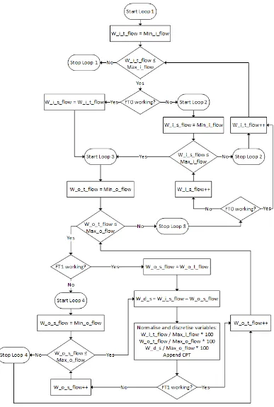
The CPTs for the nodes are derived following the arithmetic operations that have to be performed on the parent node information. For example, the CPT for the node “FT0 water – FT1” was derived by looping through all of the possible water inflow and outflow values (starting with a minimum inflow/outflow value and gradually increasing it with a selected step value until a maximum inflow/outflow value is reached) and calculating the difference between them. If both transmitters FT0 and FT1 are working, the shown information about the inflow/outflow will be the same as the true inflow/outflow. If one or both transmitters are considered to be in a failed state (failed stuck on a single reading) an additional loop is used to loop through all of the possible inflow/outflow values that the transmitter can get stuck on. This algorithm is shown in Figure 6.

Figure 6. Algorithm to generate the CPT for the node “FT0 water – FT1”

W_o_t_flow is incremented by a step value of 0.00375 and the next iteration can be started.

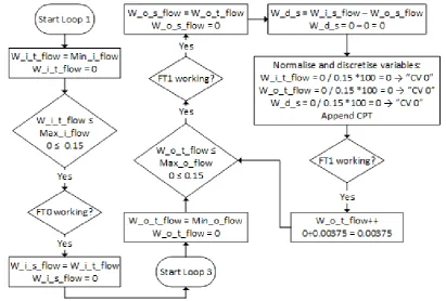
Figure 7. First iteration of the algorithm to generate the CPT for the node “FT0 water – FT1” when both transmitters are working

In the second iteration, the algorithm stays in Loop 3, where the W_o_t_flow value has just been incremented to 0.00375 and the algorithm continues as shown in Figure 8. The discrete bands of the nodes “Water inflow into separation section”, “Water outflow from separator” and “FT0 water – FT1” are found to be “CV 0”, “0 < CV ≤ 20” and “-20 ≤ CV < 0” and the corresponding entry in the CPT is incremented by +1 (see Table 10, +1 in bold italic underlined).

The W_o_t_flow is incremented by a step value of 0.00375 and the algorithm is continued until condition W_o_t_flow ≤ Max_o_flow holds. Loop 3 stops when this condition breaks and the algorithm goes back to Loop 1 where value of W_i_t_flow gets incremented by a step value. The algorithm finally terminates, when the codition W_i_t_flow > Max_i_flow is met. At each iteration, a corresponding entry in the CPT gets updated by counting the total number of times a certain discrete state of “FT0 water – FT1” is achieved given the discrete states of “Water inflow into separation section”, “Water outflow from separator”, “FT0 condition” and “FT1 condition”.

Figure 8. Second iteration of the algorithm to generate the CPT for the node “FT0 water – FT1” when both transmitters are working

For example, when both transmitters FT0 and FT1 are working and the “Water inflow into separation section” is in state “0 < CV ≤ 20” and the “Water outflow from separator” is in state “20 < CV ≤ 40”, the algorithm calculates that there are 28 differences “Water inflow into separation section – Water outflow from separator” such that the node “FT0 water – FT1” is in state “-40 ≤ CV < -20” and 36 differences when the node is in state “-20 ≤ CV < 0”. These numbers are then normed to the total number of possible differences to obtain the conditional probabilities. For instance, this gives the probability for a node “FT0 water – FT1” to be in state “-40 ≤ CV < -20” as ₂₈₊₃₆28 = 0.4375, given the states of parent nodes, as seen in Table 10. All of the CPTs in this and following BBNs are generated using the same idea.

Table 10. Part of the CPT for the node “FT0 water – FT1” for a few iterations and after algorithm finishes

Single iteration After algorithm finishes

„FT0 condition“ FT W FT W

„FT1 condition“ FT W FT W

„Water inflow into separation

section“

CV 0 CV 0 0 < CV ≤ 20

„Water outflow

from separator“ CV 0 0 < CV ≤20 20 < CV ≤ 40 CV

0 0 < CV ≤ 20 20 < CV ≤ 40 CV 0 0 < CV ≤ 20 20 < CV ≤ 40 -40 ≤ CV < -20 0 0 0 0 0 8 (1.0) 0 0 28 (0.4375)

-20 ≤ CV < 0 0 +1 0 0 8 (1.0) 0 0 28 (0.4375) 36 (0.5625)

CV 0 +1 0 0 1 0 0 0 8 (0.125) 0

3.6 BBN for the separated oil section

The separated oil section contains only separated oil flowing into the section and the separated oil outflow through valve CV2. Thus the BBN to model the control loop of separated oil level and several additional nodes to model the changes of the separated oil level in the section are used to build the BBN for the separated oil section. The light blue nodes in the BBN given in Figure 10 represent the condition of the separated oil control loop components: level transmitter LT2, controller LC2, control valve CV2 and flow transmitter FT2. The pale green nodes represent the readings obtained from transmitters LT2 and FT2. The CPTs for the “Oil level change rate in the separated oil section” and “Oil level change rate in the separated oil section indicated by LT2” are obtained using the same algorithm as described in section 3.5. Only in this case the arithmetic operations are performed with nodes “Oil inflow from the separation section” and “Oil outflow from separator” and the effect of node “LT2 state” representing the state of transmitter LT2 is considered.

Figure 10. BBN “Separated oil section” to model liquid propagation in separated oil section

3.7 BBN for the gas section

green nodes represent the readings obtained from transmitters LT3, FT0, FT3 and the combination of the two latter “FT0 gas – FT3”, as explained in section 3.3.

Figure 11. BBN “Gas section” to model gas propagation in the separator 3.8 BBN for the interactions between the sections of the TPS

The BBNs that were created previously for the individual sections of the TPS (in sections 3.5, 3.6 and 3.7) are then used as instance BBNs (identified by red rectangle for gas section, blue rectangle for separation section and brown rectangle for separated oil section in Figure 12) to create a BBN for the interactions between these sections and form a BBN for the whole TPS. Note that all of the light blue shaded nodes in Figure 12 are identical to the ones that were created for the individual sections, as well as the majority of pale green shaded nodes.

The newly created information nodes “LT1 + LT2 level changes”, “FT0 water – FT1 + FT0 oil – FT2” are used to input information into the BBN on how the volume available for the gas in the separator changes. Other information nodes “FT0 readings varied”, “FT1 readings varied”, “FT2 readings varied”, “FT3 readings varied” are used to input information into the BBN on whether there was any variability in flow transmitter readings throughout time. The individual sections are then connected in the following way:

 “Separation section” is connected to “Separated oil section” by making the output node “Flow over weir” (from “Separation section”) as a parent node of an input node “Oil inflow from the separation section” (from “Separated oil section”).

parent nodes of an input node “Change of volume for gas in the separator” in “Gas section”.

The BBN created is called “Single time slice” since it relates to the sensor readings observed during a time interval, which is called a time slice, as explained in section 3.1. Multiple instances of the “Single time slice” BBN are then joined (see section 3.9) to form a final OOBN for fault detection and diagnostics of the TPS. The number of time slices and the length of a time slice should be considered individually based on the physical properties of the separator and available computing resources. For example, if a chosen time slice is too long, by the time the failure is detected it is not possible to prevent the hazardous event. However, if a chosen time slice is too short, no changes in the readings of level transmitters can be observed for a long time due to the operating conditions of the TPS. An example of triple time slice BBN structure, which is used in the case study, is given in the next section.

Figure 12. BBN “Single time slice” for interactions between the sections of three-phase separator

Note that output nodes from BBNs “Separation section”, “Separated oil section” and “Gas section” that are not parents of any other nodes in the BBN “Single time slice” are omitted in Figure 12 due to a less complex graphical representation.

3.9 Triple time slice OOBN for fault detection and diagnostics of the TPS

“t-1=>t” which indicates the time slice number (for example “FT0 state t-3=>t-2”, “FT0 state t-3=>t-2” and “FT0 state t-1=>t”).

The instances of the single time slice BBNs are joined by connecting the condition nodes from consecutive time slices, i.e. the condition node of transmitter FT0 from a time slice t-3=>t-2 (“FT0 state t-3=>t-2” in Figure 13) is made a parent node of the identical condition node in the consecutive time slice BBN (“FT0 state t-2=>t-1” in Figure 13). This is done by assigning probabilities close to 1 (e.g. 0.99999) for the nodes to stay in the same state and probabilities close to 0 (e.g. 10-5) for the nodes to change states. For example, when the node “FT0 state t-3=>t-2” is made a parent node of “FT0 state t-2=>t-1”, a probability of 0.99999 for the node “FT0 state t-2=>t-1” to be in state “FT0 working” is set if the node “FT0 state t-3=>t-2” is in state “FT0 working”. A small probability set for the condition nodes to change states from failed to working states between time slices allows the BBN to recover from wrongly detecting a failed state of the component if new evidence provided to the BBN contradicts the current findings. An example CPT for connecting the condition nodes (“FT0 state t-3=>t-2” and “FT0 state t-2=>t-1”) between the time slices is given in Table 11.

Table 11. CPT for variable “FT0 state 2=>1”, P(“FT0 state 2=>1”| “FT0 state t-3=>t-2”)

FT0 state t-3=>t-2 FT0 working FT0 failed stuck

FT0 state t-2=>t-1 FT0 working 0.99999 0.00001

FT0 failed stuck 0.00001 0.99999

This way, the knowledge about the condition of components of TPS can be transferred through the time slices and a strong correlation can be kept for the states between the time slices.

The structure of the “Triple time slice” OOBN is given in Figure 14, indicating how the instances of BBNs are used to combine the whole OOBN. Note that the shapes in Figure 14 indicate the BBNs with identical structures.

Figure 14. Structure of the “Triple time slice” BBN for fault detection and diagnostics of three-phase separator

The OOBN created for the fault detection and diagnostics of the TPS components is used in the following way:

Step 1. Enter the sensor readings into the OOBN. If any sensor readings are present in the OOBN, shift sensor readings in information nodes back by one time slice when new sensor readings become available. For example, sensor readings entered in information node “FT1 info t-1=>t” are shifted to information node “FT1 info t-2=>t-1”.

Step 2. Update the posterior probabilities throughout the OOBN given new sensor readings.

Step 3. Track how the posterior probabilities of the condition nodes in the most recent time slice changes (nodes with a suffix “t-1=>t”) in order to detect and identify failures of components. A certain threshold has to be set for posterior probabilities so that failure modes could be detected and identified. The threshold of posterior probabilities for failure detection and diagnostics was chosen as 0.1 after several experiments with different values, thus it is a bit arbitrary and might not indicate the optimal value. It was chosen to reduce the number of false alarms, which might occur if there is a slight increase in the posterior probability, even when no failure is present.

Step 4. Check if the posterior probabilities of the condition nodes differ from the prior probabilities (set according to expert knowledge) of the same condition nodes in adjacent time slices. A certain threshold can be set in order to ignore very small differences between the prior and posterior probabilities. For example, if the posterior probabilities of condition node “FT0 state t-2=>t-1” differ only slightly from the prior probabilities of condition node “FT0 state t-3=>t-2”, the difference is ignored. The threshold for the difference of posterior and prior probabilities of the same node in two adjacent time slices was set as 0.01. Once again, this was done after several experiments with different values and might not be an optimal value. If this threshold was not exceeded, no updating of prior probabilities was performed for the particular node.

Step 5. If the difference between posterior and prior probabilities found in Step 4 is significant, make posterior probabilities of the condition nodes as prior probabilities of the condition nodes in a previous time slice For example, the posterior probabilities of condition node “FT0 state t-2=>t-1” are set as prior probabilities of condition node “FT0 state t-3=>t-2”.

Figure 15. A flowchart of fault detection and diagnostics process with OOBN Such an approach allows conditions of components of the TPS to be monitored once sensor readings become available for all three time slices following the initial start of the monitoring.

4 Case study

To show the capabilities of the fault detection and diagnostics methodology developed, several scenarios are presented, when a simulation model of a TPS (see section 2.1) is used to generate sensor readings with failures present in the TPS. Results of the selected scenarios are presented by plotting the posterior probabilities of states of condition nodes, which relate to the failure mode considered. Moreover, if additional failures are falsely detected by the OOBN, the posterior probabilities of the states of the condition nodes representing these failures are also plotted. The posterior probabilities of a condition node are plotted as a stacked column bar chart, where the posterior probability of a certain state of condition node (representing a certain failure mode of component or working mode) is represented by an individual colour. A scenario, when a single failure mode of control valve CV2 failing closed is presented next.

4.1 Scenario 1 – Control valve CV2 failed closed

was inserted) from the start of the simulated operation of the separator. Figure 16 and Figure 17 show that the OOBN has identified two possible failure modes (CV2 failed closed and LC2 failed low), based on the readings provided. The posterior probability of CV FC failure mode of valve CV2 increased to 0.5, as can be seen in Figure 16, at the same time as the failure was inserted in the simulation model. Identical behaviour was observed for the controller LC2 (see Figure 17). This can be explained since these failure modes have the same effect (LC2 failed low and CV2 failed closed) on the operation of the separator. In both cases, valve CV2 is fully closed and prevents the oil flow out of the separator. Even though the OOBN cannot isolate the exact failure cause it detects a fault in the separator immediately, i.e. as soon as the information from the sensor readings of the TPS simulation model with the failure presence is passed on to the OOBN.

Figure 16. Posterior probabilities of the states of the node labelled “CV2 state t-1 => t”

Figure 17. Posterior probabilities of the states of the node labelled “LC2 state t-1 => t”

In the following examples the plots for the level controller failure are omitted, due to the reason that it is always identified as a possible failure mode if a control valve fails and vice versa.

4.2 Scenario 2 – Level transmitter LT1 failed stuck and control valve CV1 failed opened

Failures of level transmitter LT1 failed stuck and control valve CV1 failed open are considered in this scenario. Both failures are inserted at the same time (60 seconds after the start of the simulation) in the simulation model. The posterior probabilities of the failure modes that were identified by the OOBN are given in Figure 18 and Figure 19.

Figure 18. Posterior probabilities of the states of the node labelled “LT1 state t-1 => t”

The failure of LT1 has been identified with a slight delay, as can be seen from Figure 18 (failure occurred at 60 seconds, the posterior probability of failure mode LT FS of level transmitter LT1 increased to 1 at 80 seconds). This was due to the fact that when the failure occurred the water level was above its set point (thus associated valve CV1 was kept opened to release the excess of water) and the water inflow was the same as the maximum outflow possible through CV1. For this reason, the actual water level was not changing and therefore no change was expected in the LT1 readings. However, when the water inflow decreased, a change in LT1 reading was expected and thus the failure of LT1 being stuck was identified.

The failure of CV1 failed opened has not been identified as can be seen from Figure 19 (the posterior probability of valve CV1 being in state CV W was 1 throughout the testing duration), since the failure of the LT1 transmitter forced the valve CV1 to be fully opened and the maximum flow was expected through CV1. Thus the failure mode of CV1 becomes a hidden failure and can only be detected when the failure of LT1 is rectified.

The same two failure modes are considered next, however in this case the failure of the level transmitter occurs 60 seconds after the failure of the control valve CV1 fails open has been introduced. The posterior probabilities for these failure modes can be seen in Figure 20 and Figure 21.

Figure 20. Posterior probabilities of the states of the node labelled “LT1 state t-1 => t”

This time, the failure of LT1 has been identified as soon as it was introduced (see Figure 20, red circle is the time of the failure) since the water level was expected to decrease given the water inflow and outflow. Moreover, this time the failure of CV1 failed open has been detected (posterior probability of failure mode CV FO increased to 0.59 at 90 seconds), as can be seen from Figure 21. This can be explained by the fact that level transmitter LT1 sent a water level reading to controller LC1, which indicated that control valve CV1 has to be opened less than the maximum opening of this valve.

4.3 Scenario 3 – Control valve CV1 failed opened and level transmitter LT3 failed stuck

In the third scenario, the failures of CV1 open and LT3 stuck were inserted in the simulation model (both 60 seconds after the start of the simulation). The posterior probabilities for the states of nodes CV1 failure and LT3 failure calculated by the OOBN after the sensor readings from the simulation model were input to the OOBN are plotted in Figure 22 and Figure 23.

Figure 22. Posterior probabilities of the states of the node labelled “CV1 state t-1 => t”

As previously, the CV1 failed open was identified by the OOBN with a time lag compared to the time when it was inserted in the simulation model. As can be seen from Figure 22 the failure occurred at 60 seconds and the posterior probability of CV FO increased to 0.59 at 90 seconds. This happened for the same reason as in the previous example, i.e. the water level was above the set point and valve CV1 was expected to be fully open. As soon as such expectation has changed, the CV1 open failure mode was identified.

Figure 23. Posterior probabilities of the states of the node labelled “LT3 state t-1 => t”

5 Conclusions and future work

In this study, several novel aspects were proposed for the fault detection and diagnostics of a three-phase separator. The proposed methodology using the OOBN model includes detection and diagnostics of multiple failure modes, which is a major improvement in comparison to the previously proposed approaches. Moreover, combinations of transmitter readings were proposed in order to obtain supplementary data about the processes in the separator without a need to install additional equipment.

The monitoring of the condition of the TPS components was performed by monitoring the posterior probabilities of the condition node states in the OOBN model throughout the operation of the three-phase separator. Such an approach enabled the user to be aware of the condition of the components detected earlier in the operation of the TPS.

Three scenarios of different complexities of failure present in the TPS were presented. The proposed methodology diagnosed single and multiple failures, however given certain operating conditions the model failed to detect all of the failure modes. Hidden faults were the biggest challenge, which was observed for multiple failure scenario 2 (see section 4.2). This occurred when the effects of one fault on the operation of three-phase separator cannot be observed because another component fault has happened before. In order to detect such faults additional sensors would need to be used in the system.

The research performed in this study showed the potential of the Bayesian Belief Network technique to be used as a fault detection and diagnostic tool. However, further developments of the proposed methodology would be advantageous in order to use it in practical applications.

Another important feature that has to be taken into account for the fault detection and diagnostics of the three-phase separator is the leak detection. Leaks in different places of the separator might have different effects on the liquid or pressure levels in the separator and in some cases might be a critical failure of the separator. Thus, the inclusion of the leak modelling in the BBN is recommended.

Moreover, an extensive false alarm analysis should be performed in order to find the optimal values for the two thresholds used in this study: one that is used to detect and diagnose faults and the other that is used to ignore small differences between the prior and posterior probabilities of condition nodes.

Further applications of the proposed methodology can be investigated. The proposed methodology can also be used to build BBN models for the fault detection of similar systems, for example, two inter-connected separators, free water knockout systems, desalters and other vessel based systems (having similar components: controllers, transmitters, valves) used in the oil and gas industry. It would require slight adjustment of the BBN model to the specific needs of the considered system. Acknowledgments

Dr Rasa Remenyte-Prescott is the Lloyd’s Register Foundation* Lecturer in Risk and Reliability Engineering at the University of Nottingham. Dr Dovile Rama is the Network Rail Research Fellow in Asset management. John Andrews is the Royal Academy of Engineering and Network Rail Professor of Infrastructure Asset Management. He is also Director of Lloyd's Register Foundation* for Risk and Reliability Engineering at the University of Nottingham. They gratefully acknowledge the support of these organizations.

References

1. U.S. Energy Information Administration. International Energy Statistics. 2013.

2. Chan CW. An expert decision support system for monitoring and diagnosis of petroleum production and separation processes. Expert Syst Appl. 2005; 29: 131-43.

3. Roverso D. Plant diagnostics by transient classification: The ALADDIN approach. International Journal of Intelligent Systems. 2002; 17: 767-90.

4. Omana M and Taylor JH. Fault Detection and Isolation Using the Generalized Parity Vector Technique in the Absence of an a Priori Mathematical Model. Control Applications, 2007 CCA 2007 IEEE

International Conference on. 2007, p. 970-5.

5. Taylor JH and Omana M. Fault Detection, Isolation and Accommodation Using the Generalized Parity Vector Technique. In: Chung MJ and Misra P, (eds.). Proceedings of the 17th IFAC World Congress, 2008. COEX, South Korea 2008, p. 1914-21.

6. Gao Q, Han M, Hu S-l and Dong H-j. Design of Fault Diagnosis System of FPSO Production Process Based on MSPCA. Information

Assurance and Security, 2009 IAS '09 Fifth International Conference on.

2009, p. 729-33.

7. Dias AC, Bhaya A and Kaszkurewicz E. Fault Diagnosis in an Oil Production Plant Prototype Using a Diagnostic Model Processor. American

Control Conference, 1993. 1993, p. 107-11.

8. Afonso PAFNA, Ferreira JML and Castro JAAM. Sensor Fault Detection and Identification in a Pilot Plant Under Process Control.

Chemical Engineering Research and Design. 1998; 76: 490-8.

9. Kinnaert M, Vrančić D, Denolin E, Juričić Đ and Petrovčić J. Model-based fault detection and isolation for a gas–liquid separation unit.

Control Engineering Practice. 2000; 8: 1273-83.

10. Al-Hajri EM and Rossiter JA. A unified frame work for oil producing stations using Petri nets. Control 2010, UKACC International Conference on. 2010, p. 1-8.

11. Arnold K and Stewart M. Chapter 5 - Three-Phase Oil and Water Separation. In: Stewart KA, (ed.). Surface Production Operations (Third

Edition). Burlington: Gulf Professional Publishing, 2008, p. 244-315.

12. Svrcek WY, Mahoney DP and Young BR. A Real-Time Approach to

Process Control. John Wiley \\& Sons, 2006.

13. Jensen FV and Nielsen TD. Bayesian Networks and Decision Graphs. Second Edition ed.: Springer, 2007.

14. Koller D and Pfeffer A. Object-oriented Bayesian networks.

Proceedings of the Thirteenth conference on Uncertainty in artificial