Back Propagation Network

(1)

RC Chakraborty, www.myreaders.info

Back Propagation Network : Soft Computing Course Lecture 15 – 20, notes, slides www.myreaders.info/ , RC Chakraborty, e-mail [email protected] , Aug. 10, 2010 http://www.myreaders.info/html/soft_computing.html

Back Propagation Network

Soft Computing

www.myreaders.info

Return to Website

Back-Propagation Network, topics : Background, what is back-prop network ? learning AND function, simple learning machines - Error measure , Perceptron learning rule, Hidden Layer, XOR problem.

Back-Propagation Learning : learning by example, multi-layer feed-forward back-propagation network, computation in input, hidden and output layers, error calculation. Back-propagation algorithm for training network - basic loop structure, step-by-step procedure, numerical example.

(2)

Back Propagation Network Soft Computing

Topics

(Lectures 15, 16, 17, 18, 19, 20 6 hours) Slides 1. Back-Propagation Network - Background

What is back-prop network ?; Learning : AND function; Simple learning machines - Error measure , Perceptron learning rule ; Hidden Layer , XOR problem.

03-11

2. Back-Propagation Learning - learning by example

Multi-layer Feed-forward Back-propagation network; Computation of Input, Hidden and Output layers ; Calculation of Error.

12-16

3. Back-Propagation Algorithm

Algorithm for training Network - Basic loop structure, Step-by-step procedure; Example: Training Back-prop network, Numerical example.

17-32

4. References ³³

02

(3)

Back-Propagation Network

What is BPN ?

• A single-layer neural network has many restrictions. This network can accomplish very limited classes of tasks.

Minsky and Papert (1969) showed that a two layer feed-forward network can overcome many restrictions, but they did not present a solution to the problem as "how to adjust the weights from input to hidden layer" ?

• An answer to this question was presented by Rumelhart, Hinton and Williams in 1986. The central idea behind this solution is that the errors for the units of the hidden layer are determined by back-propagating the errors of the units of the output layer.

This method is often called the Back-propagation learning rule.

Back-propagation can also be considered as a generalization of the delta rule for non-linear activation functions and multi-layer networks.

• Back-propagation is a systematic method of training multi-layer artificial neural networks.

03

(4)

SC - NN - BPN – Background 1. Back-Propagation Network – Background

Real world is faced with a situations where data is incomplete or noisy.

To make reasonable predictions about what is missing from the information available is a difficult task when there is no a good theory available that may to help reconstruct the missing data. It is in such situations the Back-propagation (Back-Prop) networks may provide some answers.

• A BackProp network consists of at least three layers of units : - an input layer,

- at least one intermediate hidden layer, and - an output layer.

• Typically, units are connected in a feed-forward fashion with input units fully connected to units in the hidden layer and hidden units fully connected to units in the output layer.

• When a BackProp network is cycled, an input pattern is propagated forward to the output units through the intervening input-to-hidden and hidden-to-output weights.

• The output of a BackProp network is interpreted as a classification decision.

[Continued in next slide]

04

(5)

SC - NN - BPN –Background [Continued from previous slide]

• With BackProp networks, learning occurs during a training phase.

The steps followed during learning are :

− each input pattern in a training set is applied to the input units and then propagated forward.

− the pattern of activation arriving at the output layer is compared with the correct (associated) output pattern to calculate an error signal.

− the error signal for each such target output pattern is then back-propagated from the outputs to the inputs in order to appropriately adjust the weights in each layer of the network.

− after a BackProp network has learned the correct classification for a set of inputs, it can be tested on a second set of inputs to see how well it classifies untrained patterns.

• An important consideration in applying BackProp learning is how well the network generalizes.

05

(6)

SC - NN - BPN – Background 1.1 Learning :

AND function

Implementation of AND function in the neural network.

AND X1 X2 Y

0 0 0 0 1 0 1 0 0 1 1 1

W1

Input I₁

Output O W2

Input I₂

AND function implementation

− there are 4 inequalities in the AND function and they must be satisfied.

w10 + w20 < θ , w1 0 + w2 1 < θ , w11 + w20 < θ , w1 1 + w2 1 > θ

− one possible solution :

if both weights are set to 1 and the threshold is set to 1.5, then (1)(0) + (1)(0) < 1.5 assign 0 , (1)(0) + (1)(1) < 1.5 assign 0 (1)(1) + (1)(0) < 1.5 assign 0 , (1)(1) + (1)(1) > 1.5 assign 1

Although it is straightforward to explicitly calculate a solution to the AND function problem, but the question is "how the network can learn such a solution". That is, given random values for the weights can we define an incremental procedure which will cover a set of weights which implements AND function.

06

B

C A

(7)

SC - NN - BPN – Background

• ^{Example 1}

AND Problem

Consider a simple neural network made up of two inputs connected to a single output unit.

AND X1 X2 Y

0 0 0 0 1 0 1 0 0 1 1 1

W1

Input I₁

Output O W2

Input I₂

Fig A simple two-layer network applied to the AND problem

− the output of the network is determined by calculating a weighted sum of its two inputs and comparing this value with a threshold θ.

− if the net input (net) is greater than the threshold, then the output is 1, else it is 0.

− mathematically, the computation performed by the output unit is net = w1 I1 + w2 I2 if net > θ then O = 1, otherwise O = 0.

• Example 2

Marital status and occupation In the above example 1

− the input characteristics may be : marital Status (single or married) and their occupation (pusher or bookie).

− this information is presented to the network as a 2-D binary input vector where 1st element indicates marital status (single = 0, married = 1) and 2nd element indicates occupation ( pusher = 0, bookie = 1 ).

− the output, comprise "class 0" and "class 1".

− by applying the AND operator to the inputs, we classify an individual as a member of the "class 0" only if they are both married and a bookie; that is the output is 1 only when both of the inputs are 1.

07

B

C A

(8)

SC - NN - BPN – Background 1.2 Simple Learning Machines

Rosenblatt (late 1950's) proposed learning networks called Perceptron. The task was to discover a set of connection weights which correctly classified a set of binary input vectors. The basic architecture of the perceptron is similar to the simple AND network in the previous example.

A perceptron consists of a set of input units and a single output unit.

As in the AND network, the output of the perceptron is calculated by comparing the net input net = wi Ii and a threshold θ.

If the net input is greater than the threshold θ , then the output unit is turned on , otherwise it is turned off.

To address the learning question, Rosenblatt solved two problems.

− first, defined a cost function which measured error.

− second, defined a procedure or a rule which reduced that error by appropriately adjusting each of the weights in the network.

However, the procedure (or learning rule) required to assesses the relative contribution of each weight to the total error.

The learning rule that Roseblatt developed, is based on determining the difference between the actual output of the network with the target output (0 or 1), called "error measure" which is explained in the next slide.

08

i=1

Σ

n

(9)

SC - NN - BPN – Background

• Error Measure ( learning rule )

Mentioned in the previous slide, the error measure is the difference

between actual output of the network with the target output (0 or 1).

― If the input vector is correctly classified (i.e., zero error), then the weights are left unchanged, and

the next input vector is presented.

― If the input vector is incorrectly classified (i.e., not zero error), then there are two cases to consider :

Case 1 : If the output unit is 1 but need to be 0 then

◊ the threshold is incremented by 1 (to make it less likely that the output unit would be turned on if the same input vector was presented again).

◊ If the input Ii is 0, then the corresponding weight Wi is left unchanged.

◊ If the input Ii is 1, then the corresponding weight Wi is decreased by 1.

Case 2 : If output unit is 0 but need to be 1 then the opposite changes are made.

09

(10)

SC - NN – BPN – Background

• Perceptron Learning Rule : Equations

The perceptron learning rules are govern by two equations,

− one that defines the change in the threshold and

− the other that defines change in the weights, The change in the threshold is given by

∆ θ = - (tp - op) = - dp

where p specifies the presented input pattern, op actual output of the input pattern Ipi

tp specifies the correct classification of the input pattern ie target, dp is the difference between the target and actual outputs.

The change in the weights are given by ∆ wi = (tp - op) Ipi = - dp Ipi

10

(11)

SC - NN - BPN – Background 1.3 Hidden Layer

Back-propagation is simply a way to determine the error values in hidden layers. This needs be done in order to update the weights.

The best example to explain where back-propagation can be used is the XOR problem.

Consider a simple graph shown below.

− all points on the right side of the line are +ve, therefore the output of the neuron should be +ve.

− all points on the left side of the line are –ve, therefore the output of the neuron should be –ve.

With this graph, one can make a simple table of inputs and outputs as shown below.

AND X1 X2 Y

1 1 1 1 0 0 0 1 0 0 0 0

Training a network to operate as an AND switch can be done easily through only one neuron (see previous slides)

But a XOR problem can't be solved using only one neuron.

If we want to train an XOR, we need 3 neurons, fully-connected in a feed-forward network as shown below.

XOR X1 X2 Y

1 1 0 1 0 1 0 1 1 0 0 0

X1 X2

Y

X2 X1

11

X2

+ +

― + + +

― ― + + +

― ― + +

―

― X1

― ― ― ― ―

― ― ― ―

―

B

C A

(12)

SC - NN – Back Propagation Network 2. Back Propagation Network

Learning By Example

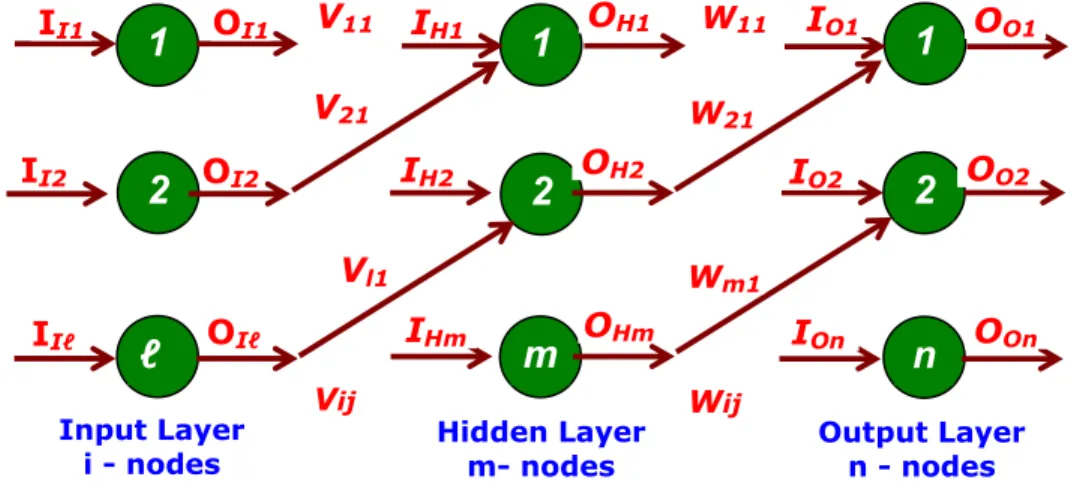
Consider the Multi-layer feed-forward back-propagation network below.

The subscripts I, H, O denotes input, hidden and output neurons.

The weight of the arc between i ^th input neuron to j ^th hidden layer is Vij . The weight of the arc between i ^th hidden neuron to j ^th out layer is W_ij

Fig Multi-layer feed-forward back-propagation network The table below indicates an 'nset' of input and out put data.

It shows ℓ inputs and the corresponding n output data.

Table : 'nset' of input and output data

No Input Ouput

I₁ I₂ . . . . _Iℓ O₁ O₂ . . . . O_n

1 0.3 0.4 . . . . 0.8 0.1 0.56 . . . . 0.82

2 : nset

In this section, over a three layer network the computation in the input, hidden and output layers are explained while the step-by-step implementation of the BPN algorithm by solving an example is illustrated in the next section.

12

Input Layer

i - nodes Hidden Layer

m- nodes Output Layer n - nodes

1 1 1

2 2 2

ℓ m n

IO1

OI1

II1 V11 IH1 OH1 W11 OO1

IO2

OI2

II2 IH2 OH2 OO2

IOn

OIℓ IHm OHm

IIℓ OOn

Wm1

Vl1

V21 W₂₁

Wij

Vij

(13)

SC - NN – Back Propagation Network 2.1 Computation of Input, Hidden and Output Layers

(Ref.Previous slide, Fig. Multi-layer feed-forward back-propagation network)

• Input Layer Computation

Consider linear activation function.

If the output of the input layer is the input of the input layer and the transfer function is 1, then

{ O }I = { I }I

ℓ x 1 ℓ x 1 (denotes matrix row, column size)

The hidden neurons are connected by synapses to the input neurons.

- Let V_ij be the weight of the arc between i^th input neuron to j^th hidden layer.

- The input to the hidden neuron is the weighted sum of the outputs of the input neurons. Thus the equation

IHp = V1p OÎ1 + V2p OÎ2 + . . . . + V1p OÎℓ where (p =1, 2, 3 . . , m) denotes weight matrix or connectivity matrix between input neurons and a hidden neurons as [ V ].

we can get an input to the hidden neuron as ℓ x m { I }H = [ V ]^T { O }I

m x 1 m x ℓ ℓ x 1 (denotes matrix row, column size)

13

(14)

SC - NN – Back Propagation Network

• Hidden Layer Computation

Shown below the p^th neuron of the hidden layer. It has input from the output of the input neurons layers. If we consider transfer function as sigmoidal function then the output of the p^th hidden neuron is given by

where ^O^Hp is the output of the p^th hidden neuron, IHp is the input of the p^th hidden neuron, and θHP is the threshold of the p^th neuron;

Note : a non zero threshold neuron, is computationally equivalent to an input that is always held at -1 and the non-zero threshold becomes the connecting weight value as shown in Fig. below.

Fig. Example of Treating threshold in hidden layer

Note : the threshold is not treated as shown in the Fig (left); the outputs of the hidden neuron are given by the above equation.

Treating each component of the input of the hidden neuron separately, we get the outputs of the hidden neuron as given by above equation .

The input to the output neuron is the weighted sum of the outputs of the hidden neurons. Accordingly, Ioq the input to the q^th output neuron is given by the equation

Ioq = W1q OH1 +W2q OH2 +. . . . + Wmq OHm , where (q =1, 2, 3 . . , n)

It denotes weight matrix or connectivity matrix between hidden neurons and output neurons as [ W ], we can get input to output neuron as

{ I }O = [ W]^T { O }H

n x 1 n x m m x 1 (denotes matrix row, column size)

14

1 OHp =

( 1 + e ^-λ^(I^HP^{– θ}^HP⁾)

1 { O }H =

( 1 + e ^{-λ (I}^HP^{– θ}^HP⁾)

– – – –

θHP

V3p

V2p

Vℓp

V1p

p

OI1

II1 1

OI2

II2 2

OI3

II3 3

OIℓ

IIℓ ℓ

OIO = -1 IIO = -1

O

(15)

SC - NN – Back Propagation Network

• Output Layer Computation

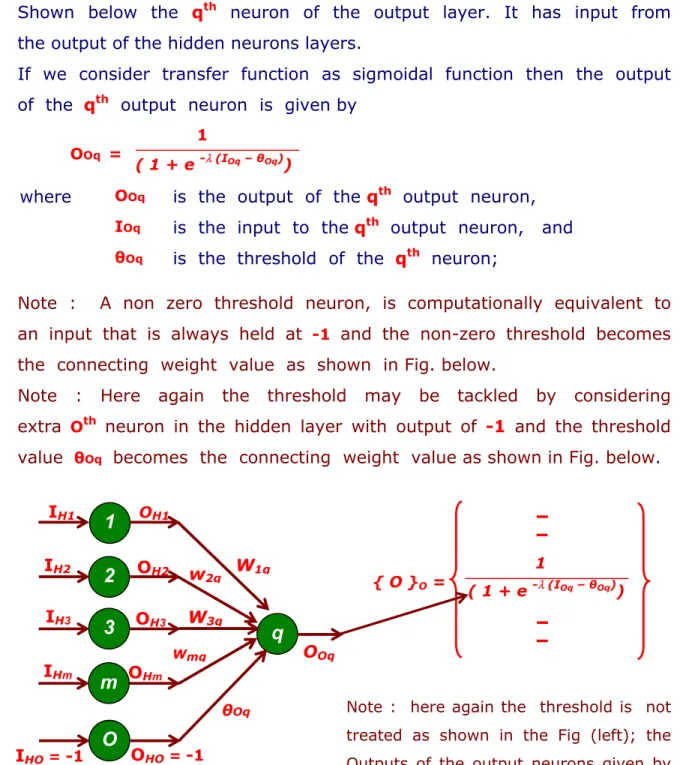
Shown below the q^th neuron of the output layer. It has input from the output of the hidden neurons layers.

If we consider transfer function as sigmoidal function then the output of the q^th output neuron is given by

where ^O^Oq is the output of the q^th output neuron, IOq is the input to theq^th output neuron, and θOq is the threshold of the q^th neuron;

Note : A non zero threshold neuron, is computationally equivalent to an input that is always held at -1 and the non-zero threshold becomes the connecting weight value as shown in Fig. below.

Note : Here again the threshold may be tackled by considering extra O^th neuron in the hidden layer with output of -1 and the threshold value θOq becomes the connecting weight value as shown in Fig. below.

Fig. Example of Treating threshold in output layer

Note : here again the threshold is not treated as shown in the Fig (left); the Outputs of the output neurons given by the above equation.

15

1 OOq =

( 1 + e ^{-λ (I}^Oq^{– θ}^Oq⁾)

1 { O }O =

( 1 + e ^{-λ (I}^Oq^{– θ}^Oq⁾)

– – – –

q

θOq

W3q

w2q

W_mq

W1q

OOq

OH1

IH1 1

OH2

IH2 2

OH3

IH3 3

OHm

IHm m

OHO = -1

IHO = -1 O

(16)

SC - NN – Back Propagation Network 2.2 Calculation of Error

(refer the earlier slides - Fig. "Multi-layer feed-forward back-propagation network"

and a table indicating an 'nset' of input and out put data for the purpose of training)

Consider any r^th output neuron. For the target out value T, mentioned in the table- 'nset' of input and output data" for the purpose of training, calculate output O .

The error norm in output for the r^th output neuron is E¹^r = (1/2) e²^r = (1/2) (T –O)²

where E¹^r is 1/2 of the second norm of the error e^r in the r^th neuron for the given training pattern.

e²^r is the square of the error, considered to make it independent of sign +ve or –ve , ie consider only the absolute value.

The Euclidean norm of errorE¹ for the first training pattern is given by E¹ = (1/2) (T^or - O^or )²

This error function is for one training pattern. If we use the same technique for all the training pattern, we get

E (V, W) = E ^j (V, W, I)

where E is error function depends on m ( 1 + n) weights of [W] and [V].

All that is stated is an optimization problem solving, where the objective or cost function is usually defined to be maximized or minimized with respect to a set of parameters. In this case, the network parameters that optimize the error function E over the 'nset' of pattern sets [I ^nset , t^nset ] are synaptic weight values [ V ] and [ W ] whose sizes are

[ V ] and [ W ] ℓ x m m x n

16

r=1

Σ

n

r=1

Σ

nset

(17)

SC - NN - BPN – Algorithm 3. Back-Propagation Algorithm

The benefits of hidden layer neurons have been explained. The hidden layer allows ANN to develop its own internal representation of input-output mapping. The complex internal representation capability allows the hierarchical network to learn any mapping and not just the linearly separable ones.

The step-by-step algorithm for the training of Back-propagation network is presented in next few slides. The network is the same , illustrated before, has a three layer. The input layer is with ℓ nodes, the hidden layer with m nodes and the output layer with n nodes. An example for training a BPN with five training set have been shown for better understanding.

17

(18)

SC - NN - BPN – Algorithm 3.1 Algorithm for Training Network

The basic algorithm loop structure, and the step by step procedure of Back- propagation algorithm are illustrated in next few slides.

• Basic algorithm loop structure Initialize the weights

Repeat

For each training pattern "Train on that pattern"

End

Until the error is acceptably low.

18

(19)

SC - NN - BPN – Algorithm

• Back-Propagation Algorithm - Step-by-step procedure

■ Step 1 :

Normalize the I/P and O/P with respect to their maximum values.

For each training pair, assume that in normalized form there are ℓ inputs given by { I }I and

ℓ x 1 n outputs given by { O}O n x 1

■ Step 2 :

Assume that the number of neurons in the hidden layers lie between 1 < m < 21

19

(20)

■ Step 3 :

Let [ V ] represents the weights of synapses connecting input neuron and hidden neuron

Let [ W ] represents the weights of synapses connecting hidden neuron and output neuron

Initialize the weights to small random values usually from -1 to +1;

[ V ] ⁰ = [ random weights ] [ W ] ⁰ = [ random weights ] [ ∆ V ] ⁰ = [ ∆ W ] ⁰ = [ 0 ]

For general problems λ can be assumed as 1 and threshold value as 0.

20

(21)

■ Step 4 :

For training data, we need to present one set of inputs and outputs.

Present the pattern as inputs to the input layer { I }I .

then by using linear activation function, the output of the input layer may be evaluated as

{ O }I = { I }I ℓ x 1 ℓ x 1

■ Step 5 :

Compute the inputs to the hidden layers by multiplying corresponding weights of synapses as

{ I }H = [ V]^T { O }I m x 1 m x ℓ ℓ x 1

■ Step 6 :

Let the hidden layer units, evaluate the output using the sigmoidal function as

m x 1

21

1 { O }H =

( 1 + e ^{- (I}^Hi⁾)

–– ––

(22)

■ Step 7 :

Compute the inputs to the output layers by multiplying corresponding weights of synapses as

{ I }O = [ W]^T { O }H n x 1 n x m m x 1

■ Step 8 :

Let the output layer units, evaluate the output using sigmoidal function as

Note : This output is the network output

22

1 { O }O =

( 1 + e ^{- (I}^Oj⁾)

–– ––

(23)

■ Step 9 :

Calculate the error using the difference between the network output and the desired output as for the j ^th training set as

E^P =

■ Step 10 :

Find a term { d } as

n x 1

23

√^∑^(T^j^-^O^oj⁾²

n

{ d } = (Tk–OOk)OOk (1 – OOk )

–– ––

(24)

■ Step 11 :

Find [ Y ] matrix as

[ Y ] = { O }H 〈 d 〉 m x n m x 1 1 x n

■ Step 12 :

Find [ ∆ W ]^{t +1} = α [ ∆ W ]^t + η^{[ Y ]}

m x n m x n m x n

■ Step 13 :

Find { e } = [ W ] { d } m x 1 m x n n x 1

m x 1 m x 1 Find [ X ] matrix as

[ X ] = { O }I 〈 d* 〉 = { I }I 〈 d* 〉 1 x m ℓ x 1 1 x m ℓ x 1 1 x m

24

(OHi) (1 – OHi ) { d* } =

–– ––

ei

(25)

■ Step 14 :

Find [ ∆ V ]^{t +1} = α [ ∆ V ]^t + η^{[ X ]}

1 x m 1 x m 1 x m

■ Step 15 :

Find [ V ]^{t +1} = [V ]^t + [ ∆ V ]^{t +1}

[ W ]^{t +1} = [W ]^t + [ ∆ W ]^{t +1}

■ Step 16 :

Find error rate as

∑ Ep

error rate =

nset

■ Step 17 :

Repeat steps 4 to 16 until the convergence in the error rate is less than the tolerance value

■ End of Algorithm

Note : The implementation of this algorithm, step-by-step 1 to 17, assuming one example for training BackProp Network is illustrated in the next section.

25

(26)

SC - NN - BPN – Algorithm 3.2 Example : Training Back-Prop Network

• Problem :

Consider a typical problem where there are 5 training sets.

Table : Training sets

S. No. Input Output

I1 I2 O

1 0.4 -0.7 0.1

2 0.3 -0.5 0.05

3 0.6 0.1 0.3

4 0.2 0.4 0.25

5 0.1 -0.2 0.12

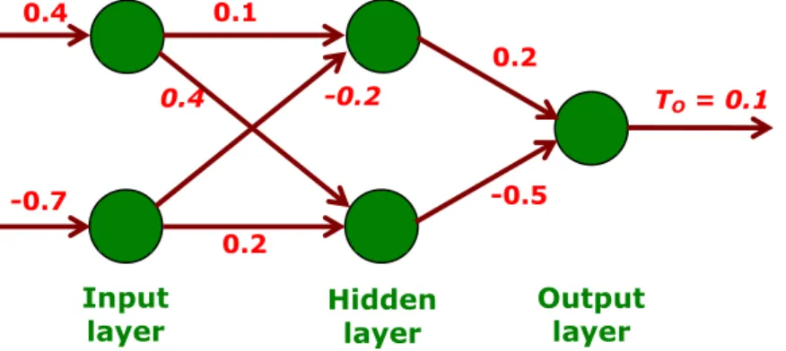
In this problem,

- there are two inputs and one output.

- the values lie between -1 and +1 i.e., no need to normalize the values.

- assume two neurons in the hidden layers.

- the NN architecture is shown in the Fig. below.

Fig. Multi layer feed forward neural network (MFNN) architecture with data of the first training set

The solution to problem are stated step-by-step in the subsequent slides.

26

0.2

0.4 -0.2 TO = 0.1

0.4 0.1

0.2

-0.7 -0.5

Input

layer Hidden

layer Output layer

(27)

■ Step 1 : Input the first training set data (ref eq. of step 1)

from training set s.no 1

■ Step 2 : Initialize the weights as (ref eq. of step 3 & Fig)

;

from fig initialization from fig initialization

■ Step 3 : Find { I }H = [ V]^T { O }I as (ref eq. of step 5)

{ I }H

Values from step 1 & 2

27

{ O }I = ℓ x 1

{ I }I =

ℓ x 1

0.4 -0.7

2 x 1

[ V ] ⁰ =

0.1 0.4

-0.2 0.2

2x2

[ W ]⁰ =

0.2 -0.5

2 x1

0.1 -0.2

-0.4 0.2

0.4 -0.7

= ^0.18

0.02

=

(28)

■ Step 4 : (ref eq. of step 6)

Values from step 3 values

28

1

( 1 + e ^{- (0.18)})

1

( 1 + e ^{- (0.02)})

{ O }H = 0.5448

0.505

=

(29)

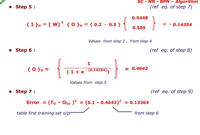
■ Step 5 : (ref eq. of step 7)

{ I }O = [ W]^T { O }H = ( 0.2 - 0.5 ) = - ^0.14354

Values from step 2 , from step 4

Values from step 5

■ Step 7 : (ref eq. of step 9) Error = (TO – OO1 )² = (0.1 – 0.4642)² = 0.13264

table first training set o/p from step 6

29

0.5448

0.505

1

( 1 + e - (0.14354))

{ O }O = = ^0.4642

(30)

■ Step 8 : (ref eq. of step 10)

d = (TO – OO1 ) ( OO1 ) (1 – OO1 )

= (0.1 – 0.4642) (0.4642) ( 0.5358) = – 0.09058 Training o/p all from step 6

(ref eq. of step 11)

[ Y ] = { O }H (d ) = (– 0.09058) =

from values at step 4 from values at step 8 above

[ ∆ W ]¹ = α [ ∆ W ]⁰ + η^{[ Y ]}^assume^{η =0.6}

=

from values at step 2 & step 8 above

{ e } = [ W ] { d } = (– 0.09058) =

from values at step 8 above

from values at step 2 30

0.5448

0.505

–0.0493

–0.0457

–0.02958

–0.02742

0.2 -0.5

–0.018116

–0.04529

(31)

■ Step 11 : (ref eq. of step 13)

{ d* } = =

from values at step 10 at step 4 at step 8

[ X ] = { O }I ( d* ) = ( – 0.00449 0.01132)

from values at step 1 from values at step 11 above

=

[ ∆ V ]¹ = α^[∆ V ]⁰ + η^{[ X ]}⁼

from values at step 2 & step 8 above

31

(–0.018116) (0.5448) (1- 0.5448)

(0.04529) (0.505) ( 1 – 0.505)

–0.00449

–0.01132

0.4 -0.7

– 0.001796 0.004528

0.003143 –0.007924

– 0.001077 0.002716

0.001885 –0.004754