Autonomous anatomical structure recognition using machine learning

MASTER THESIS

AUTONOMOUS

ANATOMICAL STRUCTURE

RECOGNITION USING

MACHINE LEARNING

Michiel Schuhmacher

TNW RAM

EXAMINATION COMMITTEE

Prof. Dr. I.A.M.J. Broeder, president and clinical supervisor Dr. Ir. F. van der Heijden, technical supervisor

B.J.C.C. Hessink-Sweep, MSc., process supervisor

DOCUMENT NUMBER

Acknowledgements

This research line in the clinical setting of the Meander Medical Centre at Amersfoort was set out by Prof. Dr. Ivo Broeders, to whom I want to express my gratitude for the opportunities received during my graduation research. He was approachable as a supervisor, kept the clinical goal in view, and was always willing to think along about my research.

The technical perspective was retained by my supervisor from the University of Twente, dr. ir. Ferdi van der Heijden. My thanks for his guidance on the research itself, by helping to formulate research questions and keeping perspective on the best way to achieve my research goal.

For the past two years I had excellent supervision by Bregje Hessink-Sweep, MSc. in developing professional soft skills, as well as growth on a personal level. I would never had thought self-reflection would be a skill I’ve come to enjoy to philosophize and talk about.

A special thanks goes out to Annick Faes, Fernand Maes, Thijs Dieltjens, and Wout Vekemans of Johnson & Johnson. They helped me tackle this assignment from a business perspective, analyzing what the root cause of my problem was, and helped with the practical problems when faced with implementing a machine learning algorithm.

Abstract

Introduction. Object detection algorithms are already applied to tomographical medical data (i.e. X-Ray scans), but not to video data of intra-abdominal minimally invasive surgery. This research made a start to work on anatomical structure recognition using machine learning algorithms.

Method. The YOLOv2 algorithm was applied to a dataset of 8 videos of colorectal surgery, with the goal to identify five anatomical structures (ureter, tendon, artery, white line of Toldt, colon) purely on visual information. 7 videos (6189 images) were used for training and validation, 1 video (1185 images) was used a test set, all annotated with bounding boxes around the target structures. Training parameters with the Adam optimizer were α = 0.0001 and batch size 8, trained for 100 epochs with a checkpoint on the lowest validation loss. A 3-layer LSTM network was added after the YOLOv2 algorithm for better performance, which was trained at α = 0.00001 for 300 epochs with a batch size of 32 and dropout of 0.2.

Results. The LSTM implementation failed to produce reliable results, with indications that the loss function was implemented falsely. The standalone YOLOv2 network had a mean average precision (mAP) of 43.72% on our test set, which is comparable to its performance on the standard object detection dataset COCO.

Discussion. The faulty LSTM implementation was narrowed down to probably a fault in the loss function. Annotation in medical data requires skill, anatomical background, and time, and is still difficult and inconsistent. Performance of YOLOv2 can be improved by training on a larger dataset, removing the ‘Toldt’ class, correctly implement the LSTM network, and keep testing for optimal settings in thresholds and learning parameters.

Table of contents

ABSTRACT ... II

INTRODUCTION ... 1

1.1RISE OF AI IN HEALTHCARE AND THUS SURGERY ... 1

1.2URETER RECOGNITION / PREDICTION... 1

1.3COMPUTER VISION AND OBJECT DETECTION ... 2

1.4VIDEO DATA ... 5

1.5GOAL OF RESEARCH... 7

RELATED WORK ... 8

2.1OBJECT DETECTION ALGORITHMS ... 8

2.1.1 Region-based Convolutional Neural Networks (R-CNN) ... 8

2.1.2 You Only Look Once (YOLO) ... 9

2.2RECURRENT NEURAL NETWORKS (RNN) ... 10

2.3A COMBINED CNN-RNN ARCHITECTURE ... 11

METHOD ... 12

3.1DATASET ... 12

3.2PROPOSED METHOD ... 12

3.2.1 YOLO algorithm ... 12

3.2.2 Expansion with LSTM layer as final layer ... 13

3.2.3 Loss function and evaluation metrics ... 14

3.3TRAINING ... 15

RESULTS ... 16

4.1TRAINING ... 16

4.2TEST SET ... 18

DISCUSSION ... 21

5.1FUTURE WORK ... 23

CONCLUSION ... 24

Introduction

1.1 Rise of AI in healthcare and thus surgery

As the application of artificial intelligence in the medical world steadily grows and spreads across multiple specializations, its implementation in the Operating Room (OR) seems a matter of time. Surgery has evolved in several major steps, the first of which is laparoscopic surgery in 60’s and 70’s [1]. The next game changer is the introduction of the tele-manipulator DaVinci some twenty years ago, which allows surgeons to operate from a distance, and is conventionally called robotic surgery. Actual robotic surgery, in which computers give feedback to surgeons during surgery, will change the field of surgery for the third time. Machine learning (ML) is a form of artificial intelligence most suitable to give feedback, be self-learning, and to recognize and classify new data.

The performance of ML algorithms at a specific task improves with experience. [2] As the computational power of computers surges, so does popularity of ML algorithms. The ability to process large amounts of data in short times nowadays yields the possibility for ML algorithms to quickly gain experience, which thus enhances their performance. The application of ML in the medical field is a field of interest since the dawn of computers in the 50’s – 60’s. [3] Contemporary applications are e.g. computer-aided diagnosis [4-7], lesion detection [8-10] , image annotation [11], or structure segmentation [12], all in different imaging modalities [13]. Research is more focused on tomographical imaging modalities (i.e. x-ray, CT, MRI, or US), and less on natural medical imaging modalities (i.e. endoscopies and minimally invasive surgery). A main reason is that (annotated) tomography data is more readily available than natural medical video data [14].

1.2 Ureter recognition / prediction

In abdominal surgery the organs and anatomical structures are not fixed in their position. Instead, these organs have a patient-specific anatomical variation, they vary with respiratory, cardiac, or bowel movement, or are manipulated by the surgeon during a procedure. The larger spatial and anatomical variation of the abdominal structures makes it more difficult to find inter-structural relations. So, even larger and more complex training data sets are needed for training ML algorithms. Though these variations have a negative effect on the efficiency of ML algorithms, it also provides the clinical relevance.

The ureter, the connection between a kidney and the bladder, has a relatively stable position and almost no patient-specific anatomical variation. That does not mean that the ureter is clearly visible during minimally invasive surgery. The sigmoid colon passes over the middle part of the ureter, and as the ureter lies retroperitoneal it can be obscured by adhesions, fatty tissue, or the peritoneum. This can cause its localization during surgery to be complex. All the while ureter localization is an obligated step during various colorectal and gynecological surgeries, to ensure that there is no ureteral damage. As the ureter is not visible at the start of surgery, that means the surgeon has to carefully look for ureter so as to work around it. To autonomously recognize the ureter, and perhaps even guide the surgeon to the ureter, means the surgeon can work faster and more secure.

Iatrogenic ureter damage is not detected intraoperatively in 50-91.4% of the cases [18, 24-26]. Also, as the symptoms are indistinct, the diagnosis duration can take days to several weeks [27]. Treatment of ureteral complications is almost always via reintervention, in 43.3-77.6% of the cases a laparotomy is the mode of repair [24]. Even if the diagnosis was made intraoperatively, the conversion rate is 33.3% [24] and in all cases the surgery duration is prolonged. [26]

1.3 Computer vision and object detection

Computer vision is an old division of computer science, originating in the late 1960’s. The rise of AI applications also occurred within computer vision research. Nowadays, AI applications in computer vision problems can be subdivided in three main subdomains, from a coarse to fine inference based on the level of data annotation (Table 1).

Table 1. Computer vision subdomains and their annotation level.

Annotation level Subdomain

Image level Image classification

Bounding box level Object detection

Pixel level Semantic segmentation

Annotating the whole image, a bounding box within the image, or each pixel of the image, determines what kind of output you get, namely the same as the input. While semantic segmentation is the most precise and is becoming more and more common, it still has some major downfalls. Annotating the data this way is extremely time-consuming, training the network is computational expensive, and training requires large amounts of data [28].

In comparison is annotating bounding boxes relatively fast, and training is also relatively computationally inexpensive. Compared to image level annotations, bounding boxes actually localize the object. Also, the annotation times and computational resources necessary are comparable between image classification and object detection [28].

Convolutional Neural Networks (CNN) were introduced by LeCun et al. in 1998 [29], with the first implementation respectfully called the LeNet. Ever since Krizhevsky et al. [30] won the ImageNet challenge in 2012 with a CNN architecture, CNNs have become the gold standard for image classification. In general CNNs consist of four main operations: convolutions, activation, pooling, and classification.

Convolutions are the first step in CNNs. These layers extract spatial features from the input images. Filters (also called kernels) are matrices which slide over the input image. The filters compute the dot product (sum of the element-wise multiplication between filter and input image) and the result is a single element of the 2D output matrix, called the feature map. See Figure 1 for clarification. Learning a CNN means to allow the algorithm itself to determine the values for these filters, and optimize them using annotated data. Though, one still needs to guide the learning by specifying the number of filters, filter size, number of layers etcetera.

The size of the result of a convolutional layer is dependent on three variables, namely the depth, stride, and zero-padding. The depth is the number of filters used for convolution. Each filter creates an own 2D feature map, and using multiple filters thus yields multiple feature maps. Stacking these feature maps together yields a 3D feature map, dependent on the number of filters (Figure 2). The filters slide over the input image (or feature map of the previous layer), and does so with a certain step size called the stride. With a stride of 1 the filter moves 1 pixel at a time, a stride of 2 moves the filter 2 pixels over. That means have a larger stride will produce a smaller feature map. In order to retain the same size before and after convolution, the edges of the input are padded with elements of zero: zero-padding (depicted in Figure 3).

After each convolution layer the feature map passes through an activation function, most commonly used is the Rectified Linear Unit (ReLU), seen in Figure 4. ReLU replaces all negative pixel values from the feature map by zero:

g(z) = max(0, z) (1)

Figure 4. The ReLU activation function. [33]

An activation function is to introduce a non-linearity into the equation. As convolution is a linear function, adding extra layers will not affect the output if no non-linearity is introduced. Other activation functions exist, such as the tanh or sigmoid function, but ReLU has proven to work best in most cases for convolutional layers [34]. The activation function is not seen as a separate layer, but as part of the convolution layer.

The pooling layer reduces the dimensionality of each feature map. Reducing the dimensionality means reduce the number of parameters to train, which shortens training time and battles overfitting. Each feature map is downsampled independently. The most common type is max pooling, which takes the max value in the pooling window, see Figure 5. Average or sum pooling are two of the alternatives. A window slides over the input, as with convolution,

Figure 2. Each filter creates its own 2D feature map, stacking these together results in a 3D output. [32]

so one can specify the size and stride of the pooling filter. Usually a stride equal to the filter size is used.

F

Figure 5. An illustration of a maximum pooling layer. [32]

The last layer(s) of a CNN is usually a fully connected (FC) layer, meaning each node of the layer is connected to all the nodes of the input (seen in Figure 6Fout! Verwijzingsbron

niet gevonden.). The 3D output of the last pooling layer is reshaped into a 1D vector, so that it

can be used as input for the FC layer. If you use multiclass classification, the last layer will be a FC layer with the number of nodes corresponding to the number of classes, to predict a probability for each class (for binary classification this number is two). The output of the convolutional and pooling layers are high-level features of the input image. The FC layer functions to classify those features into various classes. Next to that, it is another way to introduce non-linearity into the algorithm. As a high-level feature may be good for the classification task, the combination of features might be better.

The concept of using multiple layers in a neural network is called ‘deep learning’. In CNNs it is common to use multiple convolutional plus pooling layers, followed by FC layers. The convolutional layers usually use filters of size 3x3, with a stride of 1. Throughout the layers the size of feature map is usually reduced and the number of filters increased. The pooling layer are most commonly of size 2x2, with a stride of 2. That reduces the dimensionality of each feature map by half. A schematic overview of a CNN architecture is given in Figure 7.

Figure 7. A schematic overview of a standard convolutional neural network. [35]

Learning a neural network is done through backpropagation. In the case of a CNN an image is passed forward through the network and for example a prediction for an object is made in that image. The network learns by comparing its prediction to the annotated ground truth and update its weights accordingly.

Comparing the prediction with the ground truth is done with a loss function. A loss function computes the difference between the prediction and the ground truth. The mean difference across all the training samples is called the cost. The goal of training is minimizing the cost, so the network predicts with the highest possible accuracy.

The weights of a CNN are the values of the elements of the filters. The loss function calculates the cost, and for each weight is the partial derivative of the loss function calculated, called the gradient. The neural network then updates its weights with the gradients, such that it will predict a bit better in the next iteration. Updating the weights is a process called backpropagation. So training a CNN means to update the values of the filters to obtain a filter which predicts best for your dataset.

1.4 Video data

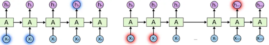
Figure 8. Overview of RNN models, copied from [36].

Each rectangle is a vector and arrows represent functions (e.g. matrix multiply). Input vectors are in red, output vectors are in blue and green vectors hold the RNN's cell state. From left to right: (1) Vanilla mode of processing without RNN, from fixed-sized input to fixed-sized output (e.g. image classification). (2) Sequence output (e.g. image captioning takes an image and outputs a sentence of words). (3) Sequence input (e.g. sentiment analysis where a sentence is classified as positive of negative). (4) Sequence input and sequence output (e.g. Machine Translation: inputs a sentence in French and outputs in English). (5) Synced sequence input and output (e.g. video classification in which each frame of the video is labelled)

RNNs can be used for several types of problems, which can be structured in the categories depicted in Figure 8. The data collected from the minimally invasive procedures are videos, and we wish to predict bounding boxes in each frame. The location of the bounding boxes in the previous frames gives information to where the bounding boxes in the current frame might be, so that makes it a many-to-many problem with synchronised sequence input and output.

RNNs are very capable in handling temporal data, because they can retain information from previous inputs, a ‘memory’ of sorts. A RNN can be seen as a chain, in which each unit is a neural network. The output of each unit is then also passed to its successor (Figure 9). A RNN processes an input xt, and computes with neural network At an output ht, similarly to vanilla

neural networks. Only, the next output of the next layer, ht+1, is not based solely on the input

xt+1, but also on the computation of the previous layer At. They are the natural architecture to

use with sequenced data.

Though in theory RNNs can make use of sequences of arbitrary length, in practice they are limited to retaining data for a few steps. The ‘long-term dependencies’ have proven difficult to learn for RNNs, due to vanishing or exploding gradients [38]. Suppose, an arbitrary unit passes its information to the next unit with a local error. When backpropagating through time to calculate the gradient to update the weights of the neural network, as one moves further backwards, this error signal in- or decreases with each timestep, and thus exponentially. The gradient is a sum of all its temporal components. In exploding gradients, the long-term components grow exponentially more than the short-term ones, blowing up the error signal. In vanishing gradients, the long-term dependencies go exponentially fast to zero, making it impossible for the model to learn a correlation with temporally distant units. [39-42] That

means the network has difficulty retaining information from far away in the sequence, and makes predictions based on only the most recent inputs from the sequence (Figure 10).

Figure 10. A RNN making prediction based on short term input (left), and long term input (right). [37]

Nowadays, a variation of the RNN is more commonly used, the Long Short-Term Memory network (LSTM). The LSTM is specifically designed to counter the vanishing (and exploding) gradient problem. More on these networks in the Related Works and Method chapters.

1.5 Goal of research

The eventual goal the research line is to predict the location of the ureter during surgery. As the ureter is not visible at the start of surgery, it is helpful to be able to guide the surgeon to the ureter for identification.

Related work

This chapter is a survey of the object detection problem in computer vision, with also an elaboration on recurrent networks. The main components of the proposed method (YOLO and LSTM, chapter 3.2) are highlighted and discussed in-depth. The combination of a CNN and a RNN, and its applications, is also discussed.

2.1 Object detection algorithms

In video data, not only increasing the accuracy of object detection algorithms is important, but also the computational efficiency in order to detect objects in real-time. Two main streams of CNN-based object detection exist, tackling the problem either as a classification or a regression problem. Classification algorithms crop the image in selected parts and feeds these cropped images to an image classifier. Regression algorithms look at the entire image and directly learn class probabilities and bounding box coordinates. Generally, classification algorithms are highly accurate, but are computationally inefficient, and vice versa for regression algorithms.

2.1.1 Region-based Convolutional Neural Networks (R-CNN)

The R-CNN method, proposed by Girshick et al. [43], is a classification algorithm and consists of three different parts. 1. It generates around 2000 category-independent region proposals using Selective Search [44]. 2. These region proposals are processed by a CNN described by Krizhevsky et al. [30], which extracts a fixed-length feature vector. 3. Then each region is classified with a set of category-specific linear Support Vector Machines. When all regions in an image are scored, a non-maximum suppression is applied for each class independently, which filters out the regions that overlap with a higher scoring region of the same class.

The first version of R-CNN was still too slow to use on real-time data, averaging around 47 seconds per image. Prompting research towards speed, Fast R-CNN [45] was developed. Fast R-CNN works faster as it does not propagate each region proposal through the entire CNN. Instead it computes a CNN-representation for the entire image once, and uses that to calculate the CNN-representation of each region proposal. Girshick et al. [45] also added bounding box regression to the neural network training, which updates the region proposals of Selective Search throughout training.

At a processing time of 2 seconds per image, Fast R-CNN came closer to real-time data processing. The latest version is Faster R-CNN [46], averaging around 0.2 seconds per image. The slowest part of its predecessors was the Selective Search, which they replaced with a small CNN called Region Proposal Network (RPN). The RPN uses a sliding window to move through the image, and at each sliding position 9 region proposals are predicted. The proposals are parameterized relative to 9 reference boxes, called anchors. That means that the RPN does not predict the bounding box coordinates directly, but instead defines the predicted bounding boxes relative to a priori defined boxes. If x, y, w, h denote the coordinates of the box center, width, and height, and x, xa, x* are for the predicted box, anchor box and ground truth box respectively

(same for y, w, h). Then the bounding box regression from an anchor box to a nearby ground truth box uses the parameterizations for the 4 coordinates as follows:

t_x= x−xa

wa , ty =

y−ya

ha , tw = log ( w

wa) , th = log ( h

ha) (2)

t_x∗ ₌ x∗−xa

wa , ty

∗ ₌y∗−ya ha , tw

∗ _{= log (}w∗ wa) , th

∗ _{= log (}h∗

2.1.2 You Only Look Once (YOLO)

In 2015, Redmon et al. [47] created the regression-based YOLO algorithm. Instead of proposing regions and classifying those regions, YOLO divides the image with a S x S grid and each grid cell predicts B bounding boxes and confidence scores for those boxes. Each bounding box consists of 5 predictions: x, y, w, h, and confidence. The (x, y) coordinates represent the center of the box relative to the bounds of the grid cell. The width and height are predicted relative to the whole image. The confidence reflects the accuracy of the bounding box and whether the bounding box contains an object (regardless of class). YOLO also predicts the classification score, C, for each box for each class in training. These two combined give a probability of each class being present in a predicted box. So in total YOLO makes S x S x (B * 5 + C) predictions. The resulting bounding boxes are compared with a probability threshold and filtered on overlap with other bounding boxes of the same class. Notice that you only run the image once through the CNN. Hence, it is possible to process images real-time. Also, processing the complete image also yields contextual information, which helps in avoiding false positives (e.g. mistaking background patches for objects). The original YOLO algorithm is exceptionally fast at 45 frames per second, and twice as accurate as other real-time algorithms of that time. Though, it still lagged behind in accuracy compared to e.g. R-CNN.

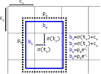
YOLOv2 focused on improving the recall and localization [48]. A variety of past ideas and novel concepts were combined to improve YOLO’s performance. The most important of those being the introduction of anchor boxes, as proposed in the Faster R-CNN algorithm. YOLOv2’s variation on the RPN still predicts the location coordinates relative to the grid cell, instead of the predicting the offset to the anchor boxes (as RPN does). YOLOv2 predicts 5 bounding boxes per grid cell in the output feature map, and each bounding box is defined by 5 coordinates: tx, ty, tw, th, and to. The cell is offset from the top left corner of the image by (cx, cy),

and the anchor box has width and height pw, ph, the predictions are visualized in Figure 11.

Still, using anchor boxes instead of directly calculating bounding box coordinates simplifies the problem and makes it easier for the network to learn. YOLOv2 works on input images of 416 x 416 pixels, and its convolutional and pooling layers downsample the image by a factor 32 to a S x S feature map of size 13 x 13. That has as extra advantage that it has a single center cell. Large objects tend to occupy the center of the image, so it helps to have a single center cell to predict these objects, instead of 4 close-by cells.

YOLOv3 is another iteration of the algorithm with incremental improvements [49]. A objectness score based on logistic regression is predicted, which is 1 when the anchor box overlaps a ground truth box more than any other anchor box. Also, instead of using a SoftMax classifier to predict the classes of a predicted bounding box, they use independent logistic classifiers for each class. A SoftMax classifier was unnecessary for good performance, and a SoftMax classifier imposes the assumption that each box has exactly one class. In some datasets a multilabel approach better suits the data (e.g. a bounding box containing the label ‘women’ and ‘person’).

2.2 Recurrent Neural Networks (RNN)

RNNs are special in that they not only map an output to a specific input, the output is dependent on the history of inputs. With the introduction of the Long Short-Term Memory (LSTM) architecture in 1997 [40] the effectiveness of RNNs was significantly changed. That is, due to vanishing or exploding error signals earlier RNNs were not able to store weights over a larger number of time steps.

The core idea of LSTMs is the cell state. Each cell takes the cell state from the previous time-step, and it removes or adds information to update the cell state. A process which is carefully regulated by structures called gates. A schematic overview of a LSTM cell is given in Figure 12.

Originally, the LSTM has separate input, forget, and output gates. The input gate controls the extent to which the cell state is updated with new values. The forget gate determines to what extent the value of the previous cell state remains in the cell. Lastly, the output gate controls the extent to which the cell state is used to compute the output activation of the cell.

The cell state of a LSTM cell is also expressed in the following equations:

c̃<t>= tanh (Wc[a<t−1>, x<t>] + bc (4)

Γ_u= σ(W_u[a<t−1>_{, x}<t>_{] + b}

u) (5)

Γ_f= σ(W_f[a<t−1>_{, x}<t>_{] + b}

f) (6)

Γ_o= σ(W_o[a<t−1>_{, x}<t>_{] + b}

o) (7)

c<t>= Γu ∗ c̃<t>+ Γf ∗ c<t−1> (8)

a<t>= Γ_o ∗ tanh c<t> (9)

In which c̃<t> is the candidate value for updating the cell state, dependent on the output of the previous cell, a<t−1>, and the current input, x<t>. Γ_u, Γ_f, Γ_o are the update, forget, and output gates, respectively, which control the cell state, c<t>.

A lot of variants on the original LSTM were proposed through the years, and a more recent one is called the Gated Recurrent Unit, proposed by Cho et al. [51]. It combines the forget and input gate into the ‘update gate’, and it merges the cell state and hidden state, amongst other changes. The result is that a GRU is a simpler unit that a LSTM unit, though they work comparably well. [52, 53]

2.3 A combined CNN-RNN architecture

A combined CNN-RNN architecture is becoming increasingly popular, especially when handling video data. While a CNN can process images for spatial information, the RNN can process the spatial information of a frame in relation to the previous frames. Performing object detection with only a CNN, thus on one image at a time, does not make use of the temporal information available in videos. In the ROLO (recurrent YOLO) architecture, proposed by Ning et al. [54], the YOLO algorithm is used to predict bounding boxes, which are then fed to a LSTM. This way the predicted bounding boxes are propagated over time.

Closely related is the use of such a model in tracking objects in video data. Multiple Object Tracking (MOT) uses object detection propagated over time to track an object, for example when it is temporarily obscured from view by a different object. While video data may seem smooth to the eye, motion blur and compression artefacts can cause substantial frame-to-frame variability [55]. Several machine learning pipelines are proposed to tackle these variabilities [55-58], though it is too early to define a clear winner.

Method

3.1 Dataset

Four different types of surgical procedures were recorded to gather the dataset, consisting of sigmoid resection, rectum resections, low anterior resections, and left-sided hemicolectomies. All procedures were colorectal, as the ureter lies in that surgical area.

In total 8 videos were collected. The videos were downsampled to a framerate of 0.5 Hz. The framerate is a trade-off between more data and similarity between the individual images. If the training samples are too much alike, the algorithm will overfit on these samples. The 8 videos yielded around 12000 raw images, including unusable ones. Annotation was done for the five target structures (ureter, colon, tendon, artery, Toldt), and the images without any target structure were excluded from training. In total, the dataset comprised of roughly 7000 images. The images were preprocessed to normalize the pixel value and reshape them to match the input size of the networks.

The CNN dataset comprised of 7 video’s in the training-validation set, and 1 video in the test set. The training-validation set was split 90%-10%. Resulting in 5570-619-1185 images per respective dataset. A validation and test set of these sizes is big enough to notice sub-percental improvements in accuracy. The dataset was shuffled randomly to battle overfitting of the network.

The LSTM requires non-shuffled data as its underlying principle is the temporal relation. The dataset was split the same way as with the CNN. A LSTM requires sequences of data instead of single images. Sequences were created in a sliding windows style, by grouping together subsequent frames (with a sequence length of 15), and then moving along one frame. So sequence 1 contained frame 1 – 15, and sequence 2 contained frame 2 – 16, etcetera. As a result, the total training-validation and the test set were both reduced with 15 frames.

3.2 Proposed method

The goal is to infer bounding boxes from image data, using a CNN to generate a spatial feature map of the image, which is fed into a RNN to capture the temporal information of the video data. The CNN is first trained on the dataset, and its performance is evaluated as a separate model. Then, the dataset is passed through the CNN to produce feature maps of the images, which are fed to the LSTM model. The LSTM model is separately trained on the same data. Training the two models separately reduces training time; the downside is that trained parameters are not shared between the two models. The two models are also evaluated separately and compared to each other.

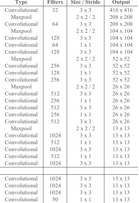
3.2.1 YOLO algorithm

Table 2. YOLOv2 model summary.

Type Filters Size / Stride Output Convolutional 32 3 x 3 416 x 416

Maxpool 2 x 2 / 2 208 x 208 Convolutional 64 3 x 3 208 x 208 Maxpool 2 x 2 / 2 104 x 104 Convolutional 128 3 x 3 104 x 104 Convolutional 64 1 x 1 104 x 104 Convolutional 128 3 x 3 104 x 104 Maxpool 2 x 2 / 2 52 x 52 Convolutional 256 3 x 3 52 x 52 Convolutional 128 1 x 1 52 x 52 Convolutional 256 3 x 3 52 x 52 Maxpool 2 x 2 / 2 26 x 26 Convolutional 512 3 x 3 26 x 26 Convolutional 256 1 x 1 26 x 26 Convolutional 512 3 x 3 26 x 26 Convolutional 256 1 x 1 26 x 26 Convolutional 512 3 x 3 26 x 26 Maxpool 2 x 2 / 2 13 x 13 Convolutional 1024 3 x 3 13 x 13 Convolutional 512 1 x 1 13 x 13 Convolutional 1024 3 x 3 13 x 13 Convolutional 512 1 x 1 13 x 13 Convolutional 1024 3 x 3 13 x 13

Convolutional 1024 3 x 3 13 x 13 Convolutional 1024 3 x 3 13 x 13 Convolutional 1024 3 x 3 13 x 13 Convolutional 50 1 x 1 13 x 13

The model output is then converted to bounding box predictions, which is subsequently filtered. The bounding boxes are first filtered on a score threshold, set to 0.6. The remaining bounding boxes are filtered on an intersection-over-union (IOU) score, set to 0.5. That means that bounding box predictions are filtered out if they overlap more than 0.5 with a bounding box pertaining to the class, with a higher confidence.

3.2.2 Expansion with LSTM layer as final layer

Table 3. LSTM model summary. None means a unspecified size, in this case this is number of training examples.

Type Units Dropout Output LSTM 1024 0.2 (None, 512) LSTM 512 0.2 (None, 512) LSTM 512 0.2 (None, 512)

Dense 8450 (None, 8450)

Dropout 8450 0.2 (None, 8450)

Dense 8450 (None, 8450)

Reshape (None, 13, 13, 50)

3.2.3 Loss function and evaluation metrics

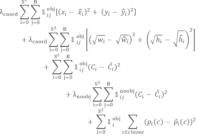
The loss function for training the two models is the same as the loss function proposed in the YOLO paper [47]. The loss function is comprised of multiple parts, based upon the sum of squared errors:

λ_coord∑ ∑ 𝟙_𝑖𝑗obj[(𝑥𝑖 − 𝑥̂𝑖)2+ (𝑦𝑖 − 𝑦̂𝑖)2] B

j=0 S2

i=0

+ λcoord∑ ∑ 𝟙𝑖𝑗

obj

[(√𝑤𝑖− √𝑤̂𝑖) 2

+ (√ℎ𝑖− √ℎ̂𝑖) 2 ] B j=0 S2 i=0

+ ∑ ∑ 𝟙_𝑖𝑗obj(𝐶_𝑖− 𝐶̂_𝑖)2

B

j=0 S2

i=0

+ λ_noobj∑ ∑ 𝟙_𝑖𝑗noobj(𝐶_𝑖− 𝐶̂_𝑖)2

B

j=0 S2

i=0

+ ∑ 𝟙_𝑖obj ∑ (𝑝_𝑖(𝑐) − 𝑝̂_𝑖(𝑐))2 𝑐∈𝑐𝑙𝑎𝑠𝑒𝑠

S2

i=0

(10)

Where 𝟙_𝑖obj denotes if the object appears in cell i, and 𝟙_𝑖𝑗obj denotes that the jth bounding box predictor in cell i is “responsible” for that prediction. The original YOLO paper [47] states some remarks about the loss function, which are reproduced here below.

In every image many grid cells do not contain any object. That pushes the confidence scores of those cells towards zero, often overpowering the gradient from cells that do contain objects. That can lead to model instability, causing training to diverge early on. This is remedied by increasing the loss from bounding box coordinate predictions and decrease the loss from confidence prediction for boxes that do not contain objects. The parameters λcoord and λnoobj

accomplish this, and are set to 5 and 1 respectively.

The sum-squared error also equally weights errors in large boxes and small boxes. Small deviations in large boxes matter less than in small boxes. To partially address this, the error metric uses the square root of the width and height, instead of directly using the width and height.

Both the CNN and LSTM model are evaluated with the mean average precision (mAP). That is the precision at different recall values, averaged for each class (the AP). These averaged precisions per class are then averaged across the classes, defining the mAP. An exemplary precision-recall curve, Figure 13, illustrates the mAP. The precision here is monotonically decreasing (in light red), meaning that the precision for a recall value r is the maximal precision of all recall values r’ > r. The average precision is the area under the curve, here shown in light blue.

Figure 13. Exemplary precision-recall curve of a class in object detection. In light red is monotonically decreasing precision. The average precision is the area under the curve, shown in light blue.

The precision and recall are defined in Equations 𝑃𝑟𝑒𝑐𝑖𝑠𝑖𝑜𝑛 = 𝑇𝑃

𝑇𝑃+𝐹𝑃 (11) and

𝑅𝑒𝑐𝑎𝑙𝑙= 𝑇𝑃

𝑇𝑃+𝐹𝑁 (12), with TP the number of true positives, FP the false positives,

and FN the false negatives. A predicted bounding box is considered a true positive when the IOU is greater than 0.5 and it shares the same label with a ground truth box. A ground truth box is only used for one predictions, to avoid multiple detections of the same object.

𝑃𝑟𝑒𝑐𝑖𝑠𝑖𝑜𝑛 = 𝑇𝑃

𝑇𝑃+𝐹𝑃 (11)

𝑅𝑒𝑐𝑎𝑙𝑙 = 𝑇𝑃

𝑇𝑃+𝐹𝑁 (12)

3.3 Training

The optimization algorithm for both networks is Adam. For the CNN the learning rate α is set at 0.0001, β1 is 0.9, β2 is 0.999, ε is 10-8, and the weight decay is not used. With a batch size of 8, the CNN was trained for 100 epochs. The initial weights of the YOLO network were trained on the Pascal VOC dataset. Early stopping was not used, but two checkpoints were used at the lowest training and validation loss. To prevent overfitting, YOLO uses batch normalization, which leads to significant improvements in convergence. It also eliminates the need for other forms of regularization. [67]

A separate test set comprised of a single annotated video, yielding a test set of 1161 images. The mAP of both networks was calculated on this test set.

Results

Two networks are trained separately: the stand-alone YOLO algorithm and a LSTM extension on YOLO. The input to the LSTM network are feature maps generated by YOLO. Both are trained on medical video data. The two networks are foremostly inter-compared to each other. Its outcomes are also compared with the results of YOLO on standard object detection dataset such as Pascal VOC and COCO. [68, 69]

The predicted bounding boxes made by the networks were first filtered on a score threshold, set at 0.6, and a IOU threshold of 0.5 with boxes of the same class (described in Section 2.1.2). The LSTM architecture performed so horribly that these thresholds were lowered to 0.05 and 0.1 respectively, on which the LSTM outputted a few comparable bounding boxes for all images. The systematic error causing this malfunctioning has not been found at the time of writing.

Table 4. Training and validation loss of the training cycles of both the YOLO and the LSTM network.

YOLO LSTM

Training loss Validation loss Training loss Validation loss

5.6328 20.3050 98.1360 97.8421

91.6159 96.2977

90.8865 96.3805

Figure 14. Training (blue) and validation (orange) loss of both networks. The YOLO network is left, the second training of the LSTM on the right.

4.1 Training

4, and plotted in Figure 14. The YOLO model uses the weights from the point of its lowest validation loss, so around epoch 4. The LSTM model also uses the weights at the minimum validation loss.

Figure 15. Example of two colon instances (annotated in light orange), they are visually quite varying.

Figure 16. Annotated image with 3 of the 5 classes present: artery, tendon, and (left and right) ureter.

4.2 Test set

The test set contained images on which the networks were not trained. For each network the true and false positives are computed, found in Figure 17. Precision-recall curves for each of the five classes were plotted based on these distributions. These precision-recall curves are found in appendix A. The mAP for each network is derived from those curves, resulting in a mAP of 43.72% for the YOLO network, and a mAP of 0.00% for the LSTM architecture. The average precision per class is found in Figure 18.

When the CNN predicted a bounding box of class ‘colon’, it did so with a high precision: 0.88. That its average precision (AP) is still the second lowest with 0.38 is caused because the CNN predicted few instances compared with the ground truths. The ground truth instances for each class are in Table 5.

Table 5. Ground truth instances in the test set.

Class: Instances: Colon 958 (944 for LSTM)

Tendon 267

Artery 225

Ureter 118

Toldt 80

Figure 17. Number of predictions per class made by the YOLO algorithm (left), and the LSTM algorithm (right).

The CNN predicted 54 + 382 = 436 instances of colon, and there were 958 ground truths annotated, that resulted in a lower AP. In comparison, the class ‘artery’ has the highest AP with 0.56, mostly because it predicted 93 + 158 = 251 bounding boxes. The CNN also predicted the most false positives in the class ‘artery’.

The LSTM predicted only a few different bounding boxes, at different locations but minimally differing in size and shape per prediction. These predictions were irrespective of input image and of prediction class. It predicted a single true positive, only based on pure luck that a ground truth box overlapped with the prediction. Figure 19 shows two images with predictions made by the LSTM. It is abundantly clear that the pipeline for predicting bounding boxes with the LSTM architecture is faulty. The resulting mAP and precision-recall curves are thus unusable.

Figure 20 shows four predictions of the ureter, made by the CNN. The false predictions can be subdivided in either an incomplete prediction (upper right) or a completely wrongful classification (bottom left). In the bottom right instance of Figure 20 the prediction is arguably a better fit than the ground truth annotation.

Discussion

The YOLOv2 algorithm is tested on several datasets, most relevant for comparison are the Pascal VOC and COCO datasets. Both focus on object detection, also expressed in the mAP. The Pascal VOC dataset has 20 annotated classes. The dataset from 2007 contains around 24,000 images, combined with the 2012 dataset its total lies around 50,000 images. [68] The COCO dataset is comprised of 200,000 images for 80 classes. [69] The performance of the YOLOv2 algorithm on these datasets, together with its performance on our dataset, are found in Table 6.

Table 6. YOLOv2 performance on different datasets. Results from [48].

Algorithm Pascal VOC 2007 Pascal VOC 2007+2012 COCO Own dataset

YOLOv2 73.4 mAP 78.6 mAP 44.0 mAP 43.7 mAP

A larger dataset (though also for more classes) does not necessarily mean a better performance, proven by the difference between YOLO’s performance on Pascal VOC and COCO. COCO is considered more difficult than Pascal VOC as the objects annotated are more heterogenous. Some objects are in the background of the image, partially obscured by other objects, and are depicted in numerous orientations. Pascal VOC tends to have the objects central to the image and clearly depicted. Our own dataset can be definitely described as a more challenging dataset than Pascal VOC, more in line with the COCO dataset. Our dataset only has 5 classes, but instances between these classes can differ heavily (see Figure 15). The objects are regularly partially obscured, smudged or blurred, or in the background (out of focus) of the image. On top of that differ the hardware settings per recorded video in terms of light source strength, robotic versus laparoscopic surgery, and type/brand of camera used in laparoscopic procedures. These are all factors which influence the performance, though it also trains a more robust algorithm which can locate structures in varying conditions.

Annotation itself is troublesome and has a flat learning curve. A lot of images are blurred, smeared, or out of focus. Recognizing anatomical structures is easier in the video data, but single stationary images are difficult. The temporal information plays a crucial role in identifying structures. For example, the ureter can be difficult to recognize, but its peristaltic movement reveals whether it actually is the ureter or something different. Also, the annotator is constantly challenged with the choice whether something is still recognizable as a structure, or whether it is too much obscured or moved out of the image. Especially when following a structure through time, and annotating it in every image, there comes a point when the structure is not recognizable anymore as the structure. Purely the temporal information from previous images hints that the structure is still in view. This inherently causes a grey area in annotation, which reflects onto the choices the algorithm makes.

Other difficulties which the annotator faces are obscuration by an instrument or another anatomical structure (e.g. fat). Does one draw a bounding boxes around the entire structure including the obscuration, or does one annotate the structure partially, or in multiple bounding boxes? Being consistent in these choices is important as it defines the dataset, and thus the performance of the algorithm.

Consistently missing structures is also a pitfall to look out for. When a lot of structures are present in a single image, it is easier to miss something. An incidental miss does not affect the algorithm, but consistently missing structures causes the algorithm to learn as not a structure, achieving the opposite of the goal.

a lot of other structures. It is an inherent disadvantage of object detection, but annotating pixels (semantic segmentation) would definitively improve performance.

The classes were chosen based on a preliminary, unpublished research into the anatomical structures present during such surgeries. The white line of Toldt was thought to be an well-defined structure, was proved not to be on stationary images. It is lateral of the colon, so the bounding boxes always overlap with the boxes of the colon. Also, it is a structure that is torn apart as one mobilizes the colon. Overall, the white line of Toldt was underrepresented in the training data. Which could be solved by adding a class weight during training. Though, Toldt is also uncommon in the test data, so the algorithm should focus to much on detecting it. It might be a good idea to remove the class altogether.

Trained on our dataset, the difference between the loss of the YOLO model on the training set and validation set is a few points, implying room for improvement. A training loss of 12 and a validation loss of 18 implies both a bias and variance available in the network. Still, the network does not overfit (when stopped on time with training), and generalizes well to new data. The variance (difference between training and validation loss) means that more training data can definitively help in its performance. More data doesn’t help per se for the bias (high training loss), though it will presumably reduce the training set error, as the dataset is still quite small for object detection standards.

No data augmentation was used on the dataset, which is also an easy option to generate more data. The anatomical structures have a quite constant locations in the images, information which is lost if data augmentation is applied.

Other options generally include trying a bigger network, training longer, or trying a different architecture. Training longer does not seem feasible, as the YOLO model started overfitting itself to training set. In this case, a bigger network and/or a different architecture is exactly what we tried with the LSTM expansion.

The pipeline for predicting bounding boxes with the LSTM network is as follow:

1. Inputting an image in the YOLO algorithm, resulting in a 13 x 13 x 50 feature map 2. Flatten the feature map to a 8450-sized feature vector

3. Sequence the feature vectors, as explained in the method (Section 3.1) 4. The sequences are fed to the LSTM network

5. The output is a 8450-sized vector, reshaped to 13 x 13 x 50

6. Post-processed the same way as with YOLO: filtering on a score threshold and IOU

The systematic error in this pipeline was narrowed down to the LSTM network itself. The feature vectors, and its sequences, are different from one to another (though they are quite alike, which is logical as the input images are visibly similar). The output from the LSTM is almost identical for each input. Different weights from training times do have influence on the output of the LSTM, but the results are still similar. The network itself was varied by changing the number of layers and the number of units per layer. All variations resulted in similar, faulty outputs. The network is trained to output a few bounding boxes as predictions, regardless of its input and the class it tried to predict.

The results of the YOLOv2 network are filtered on a score threshold of 0.6, meaning that only the better predictions remain. These bounding boxes are then compared to the ground truths, on which the mAP is based. Lowering the threshold means more predicted bounding boxes per image, but likely also in more false positives. So a tradeoff has to be made between predicting enough bounding boxes and predicting not too many, as it has direct influence on the mAP.

The classes ‘colon’ and ‘Toldt’ have the lowest AP, though they are the largest and smallest datasets, respectively. Both predict only about half as many bounding boxes as there are ground truths of those classes, making it impossible to raise above a AP of 0.5.

The predictions and the ground truths per image are matched to each other. So, only images with a ground truth box and a predicted box were included in the calculation of the mAP. Predictions in images without a ground truth were thus excluded. Including those lowers the mAP, as these are false negative predictions.

A manual survey of the false predictions, e.g. in Figure 19 and Figure 20, shows that the YOLO network does not make a lot of completely wrongful predictions. Most false predictions have a too low IOU with the ground truths, so changes in the IOU threshold also influence the mAP. Following convention, we maintained a IOU threshold of 0.5.

5.1 Future work

The adaptation of YOLO to work on medical video data worked well. Its performance can be improved by foremostly enlarging the dataset. This can be done by annotating more data, and by augmenting the existing dataset. As of yet the dataset is small in object detection terms, implying a larger dataset will boost performance. The classes with which the data is annotated can be re-evaluated. Removing the ‘Toldt’ class will speed up annotation time and increase overall performance.

The bias in the model suggests that a more complex model will help performance. This is a strong indication that the LSTM extension should be feasible. At the moment it still doesn’t work, so getting the implementation working is a second priority. The pipeline as of yet can be checked whether it contains any faulty implementations, with special regard to the loss function. Otherwise, another extension of the CNN should be considered, such as a Gated Recurrent Unit (also a type of a recurrent neural network).

Conclusion

References

1. Lau, W., C. Leow, and A.K. Li, History of endoscopic and laparoscopic surgery. World journal of surgery, 1997. 21(4): p. 444-453.

2. Mitchell, T.M., Machine learning (mcgraw-hill international editions computer science series). 1997.

3. Kononenko, I., Machine learning for medical diagnosis: history, state of the art and perspective.

Artificial Intelligence in medicine, 2001. 23(1): p. 89-109.

4. Schoepf, U.J. and P. Costello, CT angiography for diagnosis of pulmonary embolism: state of the art.

Radiology, 2004. 230(2): p. 329-337.

5. Suk, H.-I., et al., Latent feature representation with stacked auto-encoder for AD/MCI diagnosis. Brain Structure and Function, 2015. 220(2): p. 841-859.

6. Suk, H.-I., D. Shen, and A.s.D.N. Initiative, Deep learning in diagnosis of brain disorders, in Recent Progress in Brain and Cognitive Engineering. 2015, Springer. p. 203-213.

7. Suk, H.-I., et al., State-space model with deep learning for functional dynamics estimation in resting-state fMRI. NeuroImage, 2016. 129: p. 292-307.

8. Pereira, S., et al., Brain tumor segmentation using convolutional neural networks in MRI images. IEEE transactions on medical imaging, 2016. 35(5): p. 1240-1251.

9. van Tulder, G. and M. de Bruijne, Combining generative and discriminative representation learning for lung CT analysis with convolutional restricted boltzmann machines. IEEE transactions on medical imaging, 2016. 35(5): p. 1262-1272.

10. Dou, Q., et al., Automatic detection of cerebral microbleeds from MR images via 3D convolutional neural networks. IEEE transactions on medical imaging, 2016. 35(5): p. 1182-1195.

11. Shin, H.-C., et al. Learning to read chest x-rays: Recurrent neural cascade model for automated image annotation. in Proceedings of the IEEE Conference on Computer Vision and Pattern Recognition. 2016.

12. Tajbakhsh, N., et al., Convolutional neural networks for medical image analysis: Full training or fine tuning? IEEE transactions on medical imaging, 2016. 35(5): p. 1299-1312.

13. Erickson, B.J., et al., Machine learning for medical imaging. Radiographics, 2017. 37(2): p. 505-515. 14. Shen, D., G. Wu, and H.-I. Suk, Deep learning in medical image analysis. Annual review of biomedical

engineering, 2017. 19: p. 221-248.

15. Andersson, Å. and L. Bergdahl, Urologic complications following abdominoperineal resection of the rectum. Archives of Surgery, 1976. 111(9): p. 969-971.

16. Kramhøft, J., et al., Urologic complications after operations for anorectal cancer, with an evaluation of preoperative intravenous pyelography. Diseases of the Colon & Rectum, 1975. 18(2): p. 118-122. 17. Graham, J. and J. Goligher, The management of accidental injuries and deliberate resections of the

ureter during excision of the rectum. British Journal of Surgery, 1954. 42(172): p. 151-160.

18. Palaniappa, N.C., et al., Incidence of iatrogenic ureteral injury after laparoscopic colectomy. Archives of surgery, 2012. 147(3): p. 267-271.

19. Parpala-Spårman, T., et al., Increasing numbers of ureteric injuries after the introduction of laparoscopic surgery. Scandinavian journal of urology and nephrology, 2008. 42(5): p. 422-427. 20. Härkki-Siren, P., J. Sjöberg, and T. Kurki, Major complications of laparoscopy: a follow-up Finnish

study. Obstetrics & Gynecology, 1999. 94(1): p. 94-98.

21. Härkki-Sirén, P., J. Sjöberg, and A. Tiitinen, Urinary tract injuries after hysterectomy. Obstetrics & Gynecology, 1998. 92(1): p. 113-118.

22. Saidi, M.H., et al., Diagnosis and management of serious urinary complications after major operative laparoscopy. Obstetrics & Gynecology, 1996. 87(2): p. 272-276.

23. Grainger, D.A., et al., Ureteral injuries at laparoscopy: insights into diagnosis, management, and prevention. International Journal of Gynecology & Obstetrics, 1990. 33(4): p. 385-385.

24. Ostrzenski, A., B. Radolinski, and K.M. Ostrzenska, A review of laparoscopic ureteral injury in pelvic surgery. Obstetrical & gynecological survey, 2003. 58(12): p. 794-799.

25. Dandolu, V., et al., Accuracy of cystoscopy in the diagnosis of ureteral injury in benign gynecologic surgery. International Urogynecology Journal, 2003. 14(6): p. 427-431.

26. Vakili, B., et al., The incidence of urinary tract injury during hysterectomy: a prospective analysis based on universal cystoscopy. American Journal of Obstetrics & Gynecology, 2005. 192(5): p. 1599-1604.

28. Garcia-Garcia, A., et al., A review on deep learning techniques applied to semantic segmentation. arXiv preprint arXiv:1704.06857, 2017.

29. LeCun, Y., et al., Gradient-based learning applied to document recognition. Proceedings of the IEEE, 1998. 86(11): p. 2278-2324.

30. Krizhevsky, A., I. Sutskever, and G.E. Hinton. Imagenet classification with deep convolutional neural networks. in Advances in neural information processing systems. 2012.

31. Ghosh, T. What is the meaning of a filter size in a CNN? 2016; Available from: https://www.quora.com/What-is-the-meaning-of-a-filter-size-in-a-CNN.

32. Dertat, A. Applied Deep Learning - Part 4: Convolutional Neural Networks. 2017; Available from: https://towardsdatascience.com/applied-deep-learning-part-4-convolutional-neural-networks-584bc134c1e2.

33. Ujjwalkarn. An Intuitive Explanation of Convolutional Neural Networks. 2016; Available from: https://ujjwalkarn.me/2016/08/11/intuitive-explanation-convnets/.

34. Nair, V. and G.E. Hinton. Rectified linear units improve restricted boltzmann machines. in Proceedings of the 27th international conference on machine learning (ICML-10). 2010.

35. Nell, T. Digit Recogniser CNN in R Tutorial. 2018; Available from: https://www.kaggle.com/mauddib/digit-recogniser-cnn-in-r-tutorial.

36. Karpathy, A., The Unreasonable Effectiveness of Recurrent Neural Networks. 2015: Github.

37. Olah, C. Understanding LSTM Networks. 2015; Available from: http://colah.github.io/posts/2015-08-Understanding-LSTMs/.

38. Hochreiter, S., Untersuchungen zu dynamischen neuronalen Netzen. Diploma, Technische Universität München, 1991. 91(1).

39. Bengio, Y., P. Simard, and P. Frasconi, Learning long-term dependencies with gradient descent is difficult. IEEE transactions on neural networks, 1994. 5(2): p. 157-166.

40. Hochreiter, S. and J. Schmidhuber, Long short-term memory. Neural computation, 1997. 9(8): p. 1735-1780.

41. Pascanu, R., T. Mikolov, and Y. Bengio. On the difficulty of training recurrent neural networks. in

International Conference on Machine Learning. 2013.

42. Britz, D., Recurrent Neural Networks Tutorial, Part 1 - Introduction to RNNs. 2015: WildML.

43. Girshick, R., et al. Rich feature hierarchies for accurate object detection and semantic segmentation. in

Proceedings of the IEEE conference on computer vision and pattern recognition. 2014.

44. Uijlings, J.R., et al., Selective search for object recognition. International journal of computer vision, 2013. 104(2): p. 154-171.

45. Girshick, R. Fast r-cnn. in Proceedings of the IEEE international conference on computer vision. 2015. 46. Ren, S., et al. Faster r-cnn: Towards real-time object detection with region proposal networks. in

Advances in neural information processing systems. 2015.

47. Redmon, J., et al. You only look once: Unified, real-time object detection. in Proceedings of the IEEE conference on computer vision and pattern recognition. 2016.

48. Redmon, J. and A. Farhadi, YOLO9000: better, faster, stronger. arXiv preprint, 2017.

49. Redmon, J. and A. Farhadi, Yolov3: An incremental improvement. arXiv preprint arXiv:1804.02767, 2018.

50. Ng, A. Long Short-Term Memory (LSTM). Sequence Models 2018; Available from:

https://www.coursera.org/learn/nlp-sequence-models/lecture/KXoay/long-short-term-memory-lstm. 51. Cho, K., et al., Learning phrase representations using RNN encoder-decoder for statistical machine

translation. arXiv preprint arXiv:1406.1078, 2014.

52. Bahdanau, D., K. Cho, and Y. Bengio, Neural machine translation by jointly learning to align and translate. arXiv preprint arXiv:1409.0473, 2014.

53. Chung, J., et al., Empirical evaluation of gated recurrent neural networks on sequence modeling. arXiv preprint arXiv:1412.3555, 2014.

54. Ning, G., et al. Spatially supervised recurrent convolutional neural networks for visual object tracking. in Circuits and Systems (ISCAS), 2017 IEEE International Symposium on. 2017. IEEE.

55. Tripathi, S., et al., Context matters: Refining object detection in video with recurrent neural networks.

arXiv preprint arXiv:1607.04648, 2016.

56. Agarwal, A. and S. Suryavanshi, Real-Time* Multiple Object Tracking (MOT) for Autonomous Navigation. 2017.

58. Stewart, R., M. Andriluka, and A.Y. Ng. End-to-end people detection in crowded scenes. in

Proceedings of the IEEE conference on computer vision and pattern recognition. 2016.

59. Laokulrat, N., et al. Generating Video Description using Sequence-to-sequence Model with Temporal Attention. in Proceedings of COLING 2016, the 26th International Conference on Computational Linguistics: Technical Papers. 2016.

60. Diba, A., et al., Temporal 3D ConvNets: New Architecture and Transfer Learning for Video Classification. arXiv preprint arXiv:1711.08200, 2017.

61. Donahue, J., et al. Long-term recurrent convolutional networks for visual recognition and description. in Proceedings of the IEEE conference on computer vision and pattern recognition. 2015.

62. Fayyaz, M., et al., STFCN: spatio-temporal FCN for semantic video segmentation. arXiv preprint arXiv:1608.05971, 2016.

63. Sainath, T.N., et al. Convolutional, long short-term memory, fully connected deep neural networks. in

Acoustics, Speech and Signal Processing (ICASSP), 2015 IEEE International Conference on. 2015. IEEE.

64. Chan, W., et al. Listen, attend and spell: A neural network for large vocabulary conversational speech recognition. in Acoustics, Speech and Signal Processing (ICASSP), 2016 IEEE International

Conference on. 2016. IEEE.

65. Lai, S., et al. Recurrent Convolutional Neural Networks for Text Classification. in AAAI. 2015. 66. Simonyan, K. and A. Zisserman, Very deep convolutional networks for large-scale image recognition.

arXiv preprint arXiv:1409.1556, 2014.

67. Ioffe, S. and C. Szegedy, Batch normalization: Accelerating deep network training by reducing internal covariate shift. arXiv preprint arXiv:1502.03167, 2015.

68. Everingham, M., et al., The pascal visual object classes (voc) challenge. International journal of computer vision, 2010. 88(2): p. 303-338.