The resource constrained shortest path problem
implemented in a lazy functional language
Pieter H. Hartel
Department of Computer Systems, University of Amsterdam, The Netherlands, Email: [email protected]
Hugh Glaser
Department of Electronics and Computer Science, University of Southampton, England, Email: [email protected]
Abstract
The resource constrained shortest path problem is an NP-hard problem for which many ingenious algorithms have been developed. These algorithms are usually implemented in FORTRAN or another imperative programming language. We have implemented some of the simpler algorithms in a lazy functional language. Benefits accrue in the software engineering of the implementations. Our implementations have been applied to a stan-dard benchmark of data files, which is available from the Operational Research Library of Imperial College, London. The performance of the lazy functional implementations, even with the comparatively simple algorithms that we have used, is competitive with a reference FORTRAN implementation.
Keywords: Resource constrained shortest path, lazy functional programming, dy-namic programming, benchmarking.
1 Introduction
The resource constrained shortest path problem (RCSP) is to find the shortest path in a network such that certain constraints are satisfied. We consider this an interesting problem because it provides a challenge to a functional programmer. There are three reasons for this.
Firstly, RCSP is NP-hard (Handler and Zang, 1980). Good heuristics are thus required so that on a practical problem size an answer may be found in a reasonable amount of time. This makes RCSP an interesting problem in general. Because lazy functional languages are having difficulty in achieving absolute performance, RCSP is a particularly interesting problem in the lazy functional context.
1 2 3 u u u '
&
$
% '
&
$
% initial
c= 0
~ r16=~0
c= 0
~ r26=~0
c16= 0
~ r=~0
c2 6= 0
~ r=~0
final
[image:2.612.143.443.60.202.2]Placement Non-Placement
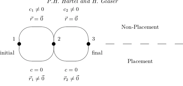
Fig. 1. Network corresponding to the knapsack problem.
The third reason for choosing RCSP is that real data sets are available via anony-mousftpfrom the Operational Research Library of Imperial College, London. Tim-ings of reference FORTRAN implementation of RCSP on these data sets are also available (Beasley and Christofides, 1989). This makes it possible to compare lazy functional implementations to a reference implementation.
We are not alone in our attempt to investigate the advantages and disadvantages of lazy functional programming when applied to implementing graph algorithms.
King and Launchbury (1993) describe implementations of depth first search and linear graph algorithms in a lazy functional language. They demonstrate that lazy functional languages are indeed useful in this area. Their chosen application area is different from ours because the complexity of their algorithms is polynomial.
Harrison and Glass (1992) use the unconstrained shortest path problem to demon-strate that standard program design techniques are applicable in a functional con-text. Their work is not concerned with efficiency.
Kashiwagi and Wise (1991) study a general schema for implementing graph al-gorithms in a lazy functional language. Their method could be applied to RCSP, but being more general it would probably not give the same performance as our implementation.
Following this introduction, Section 2 reviews some of the mathematical aspects of RCSP. In Sections 3 and 4 two implementations are discussed, for which exper-imental results are presented in Section 5. The conclusions are in Section 6.
2 A dynamic programming formulation of RCSP
To make this paper reasonably self contained, we describe the standard dynamic programming solution to RCSP. Dynamic programming is divide and conquer car-ried to its extreme: it requires solving all subproblems of a particular problem, and remembering the answers found for all the subproblems, so that they can be reused later, in case the same subproblem occurs again.
these complications makes the presentation more succinct. The simplified RCSP problem is useful. It closely corresponds to the knapsack problem. Consider the 3-node network of Figure 1. The correspondence with a 2-item knapsack is as follows: the path from nodeito nodei+ 1 along an edge in the bottom half of the diagram corresponds to placing item i with weight~ri in the knapsack. There is no cost associated with this placement. The path joining the same pair of nodes in the top half of the diagram corresponds to excluding item i from the knapsack at costci. This does not consume resource. The upperbound on the resource in the restricted RCSP problem is the capacity of the knapsack. Finding the shortest path corresponds to minimising the cost of placing items in the knapsack, and therefore maximising the profit.
The formulation of RCSP which is to follow is heavily based on that given by Beasley and Christofides (1989). However, they use a relational specification, with a logic variable to control the resource consumption. Our specification is purely functional.
Consider a DAG defined asG= (V, E), whereV is a set ofnnodes and E is a set ofmdirected edges. Nodes are labelled with natural numbers 1. . . n. An edge from a nodeito a nodej is identified by the pair (i, j). Node 1 is taken to be the initial node of a path and nodenis taken to be the final node of the path through the network.
Associated with each edge is a positive cost cij of type C and a positive k di-mensional resource vector~rij of type Rk. The ordering onRk is such that for all
~s, ~t∈Rk:
~s≤~t⇔(∀1≤i≤k·si ≤ti), where~s=hs1, . . . , skiand~t=ht1, . . . , tki
Let the number of edges along a path be thelengthof the path, let the sum of all
cij along a path be thecostof the path, and let the sum of all~rij along a path be theresourceof the path. Let anoptimalpath through the network be a path that has a minimal cost, while its resource does not exceed a given non-negative upper bound~u. Then RCSP is to find such an optimal path.
The RCSP problem can be formalised as follows. Define a pathpof lengthlfrom node 1 to nodenas a set ofl connected edges of the form:
p={(i1, i2),(i2, i3), . . . ,(il−1, il),(il, il+1)}, wherei1= 1 andil+1=n
LetP be the set of all paths from node 1 to noden. ThusP ⊂
℘
(E×E). For allp∈P, define the functionsC:P →C andR:P →Rk as follows:
C(p) = X
(i,j)∈p
cij R(p) =
X
(i,j)∈p
~rij
Then a particular pathp∈P is the resource constrained shortest path with respect to the graphGand the upper bound on the resource~uif and only if:
pRCSP~uG⇔p∈P∧(R(p)≤~u)∧(∀q∈P· R(q)≤~u)⇒ C(p)≤ C(q)
1 2 3 4 5 u u u u u
' $' $
initial c= 1
~ r=h4,0i
c= 2
~r=h0,4i
c= 3
~ r=h1,5i
c= 4
~ r=h1,0i
c= 5
~ r=h0,1i
c= 6
[image:4.612.143.428.100.207.2]~r=h1,1i final
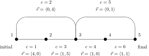
Fig. 2. Sample network, showing the costs and resources associated with each edge.
be gathered in a set, and a function could be defined, which given a graph returns the set of shortest paths. As it is often only the cost of a path satisfying RCSP that is of interest, we can define a simpler function,f∗ say, that computes just this cost.
It is convenient to use an auxiliary functionf : (V×Rk)→C, which gives the cost of the resource constrained shortest path from node 1 to a given nodej using the standard dynamic programming recursion:
f(j, ~r) = min{f(i, ~r−~rij) +cij|i∈V ∧(i, j)∈E}, ifj6= 1
f(1, ~r) =
0, if~r≥~0 ∞, otherwise
A path that consumes more than the allowed amount of resource is given a cost∞. Furthermore, min{}=∞. The optimal path has cost:
f∗
=f(n, ~u)
It can be proved by induction onnthat C(p) =f∗, wherepRCSP~
u G.
To illustrate how the functionf solves RCSP, consider the network of Figure 2. The network has 5 nodes and 6 edges; the resource vectors are of dimension 2 (i.e.
k= 2). We must now compute:
f(5, ~r) = min{f(4, ~r− h1,1i) + 6, f(3, ~r− h0,1i) + 5} ~r∈ {~u}
f(4, ~r) = min{f(3, ~r− h1,0i) + 4} ~r∈ {~u− h1,1i}
f(3, ~r) = min{f(2, ~r− h1,5i) + 3, f(1, ~r− h0,4i) + 2} ~r∈ {~u− h0,1i, ~u− h2,1i}
f(2, ~r) = min{f(1, ~r− h4,0i) + 1} ~r∈ {~u− h1,6i, ~u− h3,6i}
f(1, ~r) =
0, if~r≥~0 ∞, otherwise
~r∈ { ~u− h0,5i, ~u− h2,5i
~u− h5,6i, ~u− h7,6i}
Table 1.All possible paths through the sample network, showing the cost and the resource consumption.
path cost resource
[1,3,5] 7 h0,5i [1,2,3,5] 9 h5,6i [1,3,4,5] 12 h2,5i [1,2,3,4,5] 14 h7,6i
A simple solution to RCSP works by solving the p-th shortest path prob-lem (Christofides, 1975). The function g : V → (Rk ×C) enumerates all paths, for example in order of increasing cost:
g(j) = S
{g(i) + (~rij, cij)|i∈V ∧(i, j)∈E}, ifj6= 1
g(1) = {(~0,0)}
From the set of solutions select a feasible solution with the least cost:
g∗
= min{c|(~r, c)∈g(n)∧~0≤~r≤~u}
It can be proved by induction overn, thatf(n, ~u) = min{c|(~r, c)∈g(n)∧~0≤~r≤
~u}. Therefore,f∗=g∗.
In the network of Figure 2, the functiongcalculates the set of results as shown in Table 1, from which it is easy to select the optimal solution when given a particular value of~u. In the next two sections we will show that a lazy functional language is eminently suited to implement this strategy.
3 Initial node RCSP: discard infeasible paths at the initial node
The first step towards an efficient program is to use a dynamic programming solu-tion for the unconstrained shortest path problem, and to implement the constraints separately. The idea behind this implementation is to make each node in the graph produce a stream of paths, sorted on the cost of the path. The constraint is imple-mented by filtering out every path from a stream of paths that does not satisfy the constraint.
A solution built along these lines is not expected to be efficient, because it basi-cally enumerates all the possible paths, in order of increasing cost, until a path is found that satisfies the constraints. However, the solution has the advantage that it separates two different concerns, which is always a good idea to try first.
The lazy functional language used for the programs is Intermediate (Hartelet al., 1991), which is a variant of Miranda†(Turner, 1985). One of the extensions consists of the support for monolithic arrays withO(1) access, as in Haskell (Hudaket al., 1992). Here are two examples of array primitives. Double angular brackets are used
to denote an array thus: hhal. . . auii. All arrays are accompanied by a descriptor pairdescrl u, which holds the lower boundl and the upper bounduof the array. The first example is the functionlistarray, which turns a list into an array:
listarray :: descr→[α]→arrayα
listarray(descrl u) [xl, . . . , xu] = hhxl. . . xuii
The second example functionaccumtakes an accumulation function, an old array and a list of index/value pairs (associations). It folds new values from the list into the array using the given accumulation function:
accum :: (α→β→α)→array α→[assoc intβ]→arrayα accumf hhal. . . auii as = hhbsl. . .bsuii
where bsl = foldlf al[v|(associ v)←as;i=l] ..
.
bsu = foldlf au[v|(associ v)←as;i=u]
Returning to the solution of RCSP we first define some suitable data structures to represent the graph. A graph consists of a list of nodes and some control information. The control information gives the lowest and highest label number in the graph and the upper bound on the resource. A node consists of a label and a list of edges, and an edge contains the label of its destination as well as an integer cost and a resource vector. A resource vector is represented as a list of integer values:
> graph ::= Graph label label [resource] [node] > node ::= Node label [edge]
> edge ::= Edge label thecost [resource] > label == int
> thecost == int > resource == int
Thepathdata type has three elements: the first is the list of nodes visited between the current node and the final nodenof the network, the second component of the data type is the cost of the path, and the third component is the amount of resource consumed along the path:
> path ::= Path [label] thecost [resource]
With these data types, the dynamic programming recursion of the shortest path can be expressed using two arrays, each indexed by labels. The first arraydefault
yields a default list of paths for every node. Taking the final node of the network as an example, the list of nodes from the final node to itself should be empty, with zero cost and resource use. The array with default path lists is built by the functionsp_default. The default lists makes sure that whatever happens, a path is available for every label. The standard functionlistarray turns a list, in this case a list of repeated, identical elements, into a finite array with the given array descriptor, in this case ranging fromlotohi:
> sp_default :: graph->array [path] > sp_default (Graph lo hi upbounds nodes)
The second arraypaths_aris defined locally within the functionsp_graph. This array will contain either a real list of paths from a node to the final node of the network, or the default list, if the node is unreachable from the initial node. The graphs being traversed are acyclic, therefore it is safe for the arraypaths_arto be defined in terms of itself. This is a standard technique in lazy functional program-ming (knot tying (Bird, 1984)). In any other language one would have to resort to a topological sorting of the array, thus working out explicitly the dependencies in the network. Using a lazy functional language gives an edge over other programming paradigms in terms of the ease of coding.
The application of the standard functionaccumhere replaces all elements of the default array by new values, which will be provided by the functionsp_node:
> sp_graph :: graph->array [path]->array [path] > sp_graph (Graph lo hi upbounds nodes) default > = paths_ar
> where
> paths_ar = accum (\x y.y) default [ sp_node paths_ar n | n <- nodes ]
The structure of the data types, which describes a graph in terms of nodes, and a node in terms of edges, will now be followed closely in describing the functions that operate on these data structures. The compositionality of both data structures and functions is another powerful feature of pure functional programming.
The functionsp_nodemerges sorted lists of path lists into a single sorted path list. The paths are sorted in order of increasing cost. The constructorassocforms a pair of the node label and the merged list of paths, for the benefit of the accum
function above:
> sp_node :: array [path]->node->assoc [path] > sp_node paths_ar (Node from edges)
> = assoc from (foldr1 merge_path_cost incoming_paths) > where
> incoming_paths = sp_edge_list paths_ar edges
The list of edges associated with a node is traversed bysp_edge_list, resulting in a list of path lists:
> sp_edge_list :: array [path]->[edge]->[[path]] > sp_edge_list paths_ar edges
> = [ sp_edge paths_ar e | e <- edges ]
The last functionsp_edgebuilds a list of new paths out of a list of existing paths. To guarantee that the dynamic programming solution is properly implemented, the functionsp_edge has to have access to the local variablepaths_ar as defined in the body ofsp_graph. The arraypaths_aris therefore passed as a parameter from
sp_graph to all the intervening functions, ultimately to be used by the current functionsp_edge.
all the paths departing from nodetoto the final node, attaching the labeltoto the list of nodes already visited and updating the cost and resource. Since the resource is implemented as a list of integers, the standard functionzip2withmay be used to perform pairwise addition on the resource vectorsresources1andresources2.
> sp_edge :: array [path]->edge->[path] > sp_edge paths_ar (Edge to cost1 resources1)
> = [ Path (to:edges) (cost1+cost2) (zip2with (+) resources1 resources2) > | Path edges cost2 resources2 <- paths_ar ! to ]
The main program combines the two functionssp_graphandsp_default oper-ating on the real path array and the default path array to solve RCSP in two steps. The list of all paths from the initial node to the final node is subscripted out of the arraypaths_ar. This causes the shortest path to be computed, which is then subjected to the resource constraint test using the upperbound upbounds in the filter of the list comprehension. Should the test fail, the next best path is computed until the desired answer appears. This answer is selected by the hdfunction and the remaining solutions are ignored. Here again we use the laziness to generate a list of results separately from choosing the desired elements of the list.
> sp_main :: graph->path > sp_main g
> = hd [ Path edges cost resources
> | Path edges cost resources <- paths_ar ! lo > ; and (zip2with (>=) upbounds resources) ] > where
> (Graph lo hi upbounds nodes) = g > paths_ar = sp_graph g (sp_default g)
This completes the presentation of the shortest path program, which discards infeasible paths at the initial node. Because of this property, the program is called theinitial node RCSP. Before moving on to a more refined program, we consider some complexity issues.
3.1 An informal complexity analysis of initial node RCSP
The unconstrained shortest path program visits each edge that is reachable from the initial node exactly once. Edges that cannot be reached from the initial node will not be visited at all. This is reassuring, but not sufficient to describe the complexity in terms of elementary operations, because whilst visiting an edge, a large number of paths may have to be built.
Before discussing the real complexity issue let us have a closer look at the be-haviour of the lazy evaluation of the program. Suppose that the shortest path also satisfies the resource constraint, which as it turns out is sometimes the case in the data sets from the Operational Research Library.
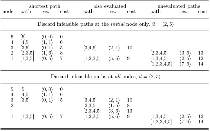
Table 2.All paths with associated resource consumption and cost on all nodes of the example network for two implementations of RCSP. All paths are placed in three categories under the assumption that only the first shortest path at node 1 (i.e. [1,3,5]) is requested. The first category gives the shortest path. The second category gives all paths that had to be evaluated to calculate the shortest path. The
third category gives all the remaining, as yet unevaluated paths.
shortest path also evaluated unevaluated paths node path res. cost path res. cost path res. cost
Discard infeasible paths at theinitialnode only,~u=h2,5i
5 [5] h0,0i 0 4 [4,5] h1,1i 6
3 [3,5] h0,1i 5 [3,4,5] h2,1i 10
2 [2,3,5] h1,6i 8 [2,3,4,5] h3,6i 13 1 [1,3,5] h0,5i 7 [1,2,3,5] h5,6i 9 [1,3,4,5] h2,5i 12 [1,2,3,4,5] h7,6i 14
Discard infeasible paths atallnodes,~u=h2,5i
5 [5] h0,0i 0 4 [4,5] h1,1i 6
3 [3,5] h0,1i 5 [3,4,5] h2,1i 10
2 [2,3,5] h1,6i 8
[2,3,4,5] h3,6i 13
1 [1,3,5] h0,5i 7 [1,2,3,5] h5,6i 9 [1,3,4,5] h2,5i 12 [1,2,3,4,5] h7,6i 14
as propagating along the edges of the graph of Figure 2. Because of the dynamic programming implementation, the shortest path on all nodes, and in particular on nodes 3 and 5 will only be computed once.
When the demand arrives at the final node, results will begin to be generated and propagated backwards towards the initial node. The precise set of evaluated paths is shown in the top half of Table 2. (The bottom half of the table will be discussed in the next section.) Also shown in the top half are the paths that are not evaluated, when only the first shortest path is demanded at the initial node. Consider as an example what happens at node 3. Here we find that path [3,5] has cost 5, which is less than the cost 10 of path [3,4,5]. Thus to form the shortest path at node 1, path [3,5] is extended to path [1,3,5] and similarly at node 2 path [3,5] is extended to path [2,3,5]. No work is done to extend path [3,4,5] at either node 1 or node 2, which explains the presence of paths [1,3,4,5] and [2,3,4,5] in the column markedunevaluated paths. Lazy evaluation is the cause of this economic pattern of evaluation.
1 t t2
G2
' $ 1 t t2 t3
G3
' $
' $
1 t t2 t3 t4 & %
G4
' $
' $
' $
1 t t2 t3 t4 t5
& % & %& %
[image:10.612.95.467.77.160.2]G5
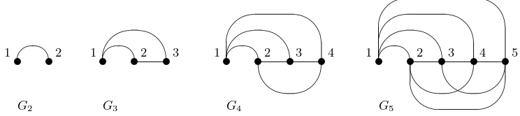
Fig. 3. The first four fully connected networks. A network withn+ 1 nodes is constructed from a network withnnodes by adding a new node and connecting this node to all other nodes. The new edges of each configuration are shown in the top half of the diagram.
particular asking for second shortest path on node 1 will only ask for the second shortest path on node 3, because the shortest path on node 2 is still available.
To investigate the worst and the best case complexity of initial node RCSP more formally consider a fully connected network (acyclic). A fully connected network with n+ 1 nodes is constructed from a fully connected network withn nodes by adding anew initialnode as follows:
• Give all nodes labelled 1. . . na new label 2. . . n+ 1. • Add a new node with label 1.
• Connect the new node to all other nodes using new edges (1,2). . .(1, n).
The construction ensures that each node is connected by a single edge to all other nodes. There is precisely one fully connected networkGn for each value of n. This can be formalised as follows:
Gn = (Vn, En)
Vn = {i | 1≤i≤n}
En = {(i, j) | 1≤i < n∧i < j ≤n}
Figure 3 shows the fully connected networksG2. . . G5. The edges in the top half of
the diagram are the new edges connecting the new node 1 to the remaining nodes. It is not difficult to show that:
| Vn | = n
| En | = Pni=1−1 n−i = n(n−1)/2
| Pn | = Pni=1−1 | Pi | = 2n−2
The number of edges|En | is thus quadratic inn and the number of paths|Pn | is exponential inn.
In the best case only the first path at node 1 needs to be generated. This causes only the first path on all other nodes to be generated. Here the laziness ensures that merging a number of sorted lists so that the head of the result becomes evaluated causes only the head of the mergeands to be evaluated. To evaluate the shortest path at any node requires a number of elementary steps to be carried out that is proportional to the number of incoming edges. Therefore in the best case, initial node RCSP is quadratic inn.
4 All node RCSP: discard infeasible paths at all nodes
The initial node RCSP program does not always have a satisfactory performance, because too many paths have to be discarded before a feasible solution appears at the initial node. The performance might be improved by discarding infeasible paths at an earlier stage – that is at all nodes of the graph – rather than at the initial node only. This new version of the program is called theall node RCSPprogram.
Lest the reader become too exited about this improved solution, remember that the evaluation of lazy functional programs is not as intuitive as it might seem. Consider the paths generated for our example shown in the bottom half of Table 2. This shows that given an upperbound of~u=h2,5i, discarding infeasible paths at node 2 causes path [2,3,4,5] to be evaluated, whereas initial node RCSP was able to avoid this. Since none of the paths at node 2 are feasible, the effort involved in generating and discarding path [2,3,4,5] is wasted. Depending on the particular graph and the precise value of the upperbound on the resource consumption, it may or may not be sensible to discard paths at all nodes. To investigate this, let us consider how to implement the discarding at each node.
The logical place to insert a filter to discard infeasible paths is in the list com-prehension of the functionsp_edge, because it is there where new paths are being built out of existing paths. If it is known that the new path could not possibly turn into a feasible solution, the new path is not generated at all. This does not affect the worst case complexity of the solution, as there may not be any path at all that can be discarded in this way. However, for some networks filtering at each node may be beneficial.
Inserting a suitable filter insp_edgerequires considerable rewriting, as the filter will need to have some information on which to base its decisions. As the decision process is associated with a particular edge, from nodenito nodenjsay, and a list of paths that pass along that edge, there are four pieces of important information:
upbounds The upperbound on the resource that any path may consume. This information is global.
left resources The minimum amount of resource that has to be available to be able to travel from the initial node to nodeni. This information is associated with a node.
resources1 The amount of resource needed to traverse the current edge, which connects node ni to node nj. This information is asso-ciated with an edge.
resources2 The amount of resource consumed along each path from the node
njto the final node of the network. This information is associated with a path.
As discarding infeasible paths requires information originating from four different sources, a new set of functions has to be written in order to propagate information. The new set of functionsrcsp_...are similar in structure to the set of functions
sp_...:
> rcsp_graph :: graph->array [resource]->array [path]->array [path] > rcsp_graph (Graph lo hi upbounds nodes) left_ar default
> = paths_ar > where
> paths_ar = accum (\x y.y) default
> [ rcsp_node upbounds left_ar paths_ar n | n <- nodes ]
> rcsp_node :: [resource]->array [resource]->array [path]->node->assoc [path] > rcsp_node upbounds left_ar paths_ar (Node from edges)
> = assoc from (foldr1 merge_path_cost incoming_paths) > where
> incoming_paths = rcsp_edge_list upbounds left_resources paths_ar edges > left_resources = left_ar ! from
> rcsp_edge_list :: [resource]->[resource]->array [path]->[edge]->[[path]] > rcsp_edge_list upbounds left_resources paths_ar edges
> = [ rcsp_edge upbounds left_resources paths_ar e | e <- edges ]
> rcsp_edge :: [resource]->[resource]->array [path]->edge->[path] > rcsp_edge upbounds left_resources paths_ar (Edge to cost1 resources1) > = [ Path (to:edges) (cost1+cost2) (zip2with (+) resources1 resources2) > | Path edges cost2 resources2 <- paths_ar ! to
> ; and (zip4with (\u x y z . u >= x+y+z)
> upbounds left_resources resources1 resources2) ]
The resources on the edge and the path (resources1and resources2) are al-ready present in the list comprehension ofsp_edge. The upper boundupboundsis available to rcsp_graph as a component of the Graph data constructor. Start-ing at rcsp_graph, the upper bound must be passed on to rcsp_node and
rcsp_edge_listuntil the upper bound arrives at rcsp_edge. The final piece of information, the arrayleft_resourceshas to follow the same route as the upper bound, thus adding one more parameter to (most of) the functions.
This leaves open the question of generating left_resources, the array that contains the minimum amount of resource necessary to travel from a particular node to the initial node. This information can be computed by the unconstrained shortest path algorithm, but in the opposite direction (Aneja et al., 1983). The most effective way to do that is by generating a new graph from the old graph, with all the edges reversed. Using a reversed graph as well as the original graph is necessary to be able efficiently to trace the nodes to which all the edges connect. In the programs that we use, both the normal and the reversed graph are built up while the data are being read from a file.
the type of the arguments and function results, in the way information arriving over different edges towards a node is combined (..._node), and in the way the information is generated (..._edge). It should be noted that the function used to combine paths (zip2with min2) takes the point wise minimum of two resource vectors.
> resource_sp_default :: graph->array [resource] > resource_sp_default (Graph lo hi upbounds nodes)
> = listarray (descr lo hi) (repeat [ 0 | i <- upbounds ])
> resource_sp_graph :: graph->array [resource]->array [resource] > resource_sp_graph (Graph lo hi upbounds nodes) default
> = rs_ar > where
> rs_ar = accum (\x y.y) default [ resource_sp_node rs_ar n | n <- nodes ]
> resource_sp_node :: array [resource]->node->assoc [resource] > resource_sp_node rs_ar (Node from edges)
> = assoc from (foldr1 (zip2with min2) (resource_sp_edge_list rs_ar edges))
> resource_sp_edge_list :: array [resource]->[edge]->[[resource]] > resource_sp_edge_list rs_ar edges
> = [ resource_sp_edge rs_ar e | e <- edges ]
> resource_sp_edge :: array [resource]->edge->[resource] > resource_sp_edge rs_ar (Edge to cost resources1) > = zip2with (+) resources1 (rs_ar ! to)
From a software engineering point of view, we should have written one set of polymorphic, higher order functions, capable of all three modes of information propagation over a graph. We have chosen not to do so because such a heavily parameterised set of functions would be harder to understand. Depending on the optimising capabilities of the compiler, there may also be a performance penalty associated with such a higher order approach.
To complete all node RCSP a main program must be provided. The function
rcsp_main follows the model of sp_main, but differs firstly because there is no longer the need to discard paths separately at the initial node, and secondly be-cause the new function needs to prepare some more information in advance. The parametersg andrev_grepresent the same graph, but in a different orientation, as discussed earlier:
> rcsp_main :: graph->graph->path > rcsp_main g rev_g
> = hd (paths_ar ! lo) > where
> (Graph lo hi upbounds nodes) = g
> paths_ar = rcsp_graph g left_ar (sp_default g)
> left_ar = resource_sp_graph rev_g (resource_sp_default rev_g)
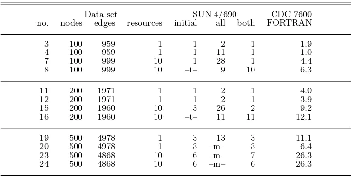
Table 3.Execution times in seconds of four implementations of RCSP with 12 data sets. The experiments marked with “–m–” ran out of memory; those marked
with “–t–” used more than 1000 seconds execution time.
Data set SUN 4/690 CDC 7600
no. nodes edges resources initial all both FORTRAN
3 100 959 1 1 2 1 1.9
4 100 959 1 1 11 1 1.0
7 100 999 10 1 28 1 4.4
8 100 999 10 –t– 9 10 6.3
11 200 1971 1 1 2 1 4.0
12 200 1971 1 1 2 1 3.9
15 200 1960 10 3 26 2 9.2
16 200 1960 10 –t– 11 11 12.1
19 500 4978 1 3 13 3 11.1
20 500 4978 1 3 –m– 3 6.4
23 500 4868 10 6 –m– 7 26.3
24 500 4868 10 6 –m– 6 26.3
5 Experiments
Table 3 shows the experimental results that have been obtained by measuring the execution time for RCSP programs applied to 12 data sets from the Operational Research Library. The table shows the number of the data set, the number of nodes, the number of edges, the number of elements in the resource vectors, followed by a row of four execution times (in seconds). Some experiments ran out of memory, because a large number of paths were generated. The entries in the table show no execution time if this happened. The last column marked FORTRAN shows the measurements reported by Beasley and Christofides (1989).
Our measurements were carried out on a SUN SPARC 4/690, running SunOS 4.1.2. Each program has 8 Mbytes of heap space available. Beasley and Christofides used a Control Data CDC 7600. Unfortunately, we have not been able to obtain a copy of the FORTRAN program, so we could not measure its perfor-mance on our SUN SPARC system. However, according to a benchmark comparison by Dongarra (1994) these systems are roughly similar in (floating point) perfor-mance: the CDC 7600 has performance of 3.3 Mflop/s and the SUN 4/600 has a performance of 4.3 Mflop/s.
The numbers reported for the SUN system in Table 3 have to be interpreted with care, because the margin of error is perhaps as large as 50%. As other researchers in the field (Hammondet al., 1993), we have observed on various occasions that an insignificant change to a program, such as the removal of the source of an unused function, caused a significant change in performance. However, the numbers do show a trend in that our best performance figures are similar to those found for FORTRAN.
infeasible paths at the initial node only. This implementation fails to deliver only on two data sets (8 and 16). Comparing the remaining entries with those in the FORTRAN column shows, that the performance of initial node RCSP is good. The reason is that in all cases except for data sets 8 and 16, a feasible path appears amongst the first few hundred shortest paths generated.
The column markedallapplies to the all node RCSP, which generally does more work than initial node RCSP. The execution times are therefore higher.
Two observations should be made regarding the all node RCSP. Firstly, as ex-pected, the number of paths generated and discarded is not so large as with the initial node RCSP. For data sets 8 and 16 execution completes without exceeding the available memory capacity.
The second observation is that for the large graphs (data sets 20–24), all node RCSP starts to run out of memory whereas initial node RCSP does not. This confirms the theory that discarding infeasible paths is sometimes wasted effort.
The column markedboth shows the result of a combination of the previous two columns. Here a new main program is used, which first usessp_graphto generate at most 10×n paths at the initial node, checking each path for feasibility. If this fails, the functionrcsp_graph is called to solve RCSP. This heuristic works well for the data sets in the Operational Research Library. It is easy to adapt to other data sets through some experimentation.
The final column marked FORTRAN reports the timings as measured by Beasley and Christofides (1989). This code used sophisticated network reduction techniques based both on the original problem and the Lagrangean relaxation (Reeves , 1993). As reported above we have had difficulty in making exact comparisons between our timings and those of Beasley and Christofides, particularly for the integer perfor-mance of the two machines involved. The evidence available to us suggests however, that it is reasonable to make a direct comparison.
6 Conclusions
We have developed three variants of a program which solves the resource constrained shortest path problem (RCSP).
Laziness helps to build compact and modular implementations of RCSP in three ways: Firstly the technique of separately generating solutions and pruning unwanted solutions has been found useful on a number of occasions. Secondly, the knot ty-ing technique allows one to postulate a solution. When this solution is elaborated, it can be used immediately. This constitutes an efficient implementation of the dynamic programming technique in a lazy functional language. Thirdly, lazy eval-uation avoids the computation of unused results in a natural way.
There are also disadvantages to purely functional programming. The first is the fact that information must be threaded explicitly from its source to its destination. Secondly, it is necessary to be careful with polymorphic, higher order functions, as there is a cost in both understandability and performance.
ar-rays, or monad based state transformers are not necessary for this problem. Purely functional, monolithic arrays withO(1) access are sufficient.
Lazy functional programs can be as efficient as FORTRAN programs when solv-ing RCSP. We found it essential to develop the implementations of RCSP startsolv-ing from first principles, rather than from an imperative implementation. In the de-velopment we have used the optimisation techniques from the literature, but not without questioning their appropriateness to the functional programming solution. Following this we are now investigating the applicability of more advanced heuris-tic techniques, including the pruning of nodes and edges and the use of Lagrangean relaxation.
7 Acknowledgements
We thank Marcel Beemster, Andy Gravell, Hugh McEvoy, Jon Mountjoy and the two referees for their comments on draft versions of the paper.
This work was supported in part by the Netherlands Organization for Scientific Research (NWO) and the British Council under grant No. BR 62-416.
References
Y. P. Aneja, V. Aggarwal, and L. P. K. Nair. Shortest chain subject to side constraints.
Networks, 13(2):295–302, 1983.
J. E. Beasley and N. Christofides. An algorithm for the resource constrained shortest path problem. Networks, 19(4):379–394, 1989.
R. S. Bird. Using circular programs to eliminate multiple traversals of data. Acta infor-matica, 21(3):239–250, 1984.
N. Christofides.Graph theory: An algorithmic approach. Academic press, New York, 1975. J. J. Dongarra. Performance of various computers using standard linear equations software. Technical report CS-89-85, Comp. Sci. Dept, Univ. of Tennessee, Knoxville, Tenessee, Feb 1994.
C. R. Reeves (ed.). Modern heuristic techniques for combinatorial problems. Blackwell Scientific publications, Oxford, England, 1993.
K. Hammond, G. L. Burn, and D. B. Howe. Spiking your caches. In K. Hammond and J. T. O’Donnell, editors,Functional programming, pages 58–68, Ayr, Scotland, Jul 1993. Springer-Verlag, Berlin.
G. Y. Handler and I. Zang. A dual algorithm for the constrained shortest path problem.
Networks, 10(4):293–310, 1980.
R. Harrison.Abstract data types in Standard ML. John Wiley & Sons, Chichester, England, 1993.
R. Harrison and C. A. Glass. Dynamic programming in a pure functional language. Technical report CSTR 92-02, Dept. of Electr. and Comp. Sci, Univ. of Southampton, England, 1992.
P. H. Hartel, H. W. Glaser, and J. M. Wild. Compilation of functional languages using flow graph analysis. Software—practice and experience, 24(2):127–173, Feb 1994. P. Hudak, S. L. Peyton Jones, and P. L. Wadler (editors). Report on the programming
language Haskell – a non-strict purely functional language, version 1.2.ACM SIGPLAN notices, 27(5):R1–R162, May 1992.
Y. Kashiwagi and D. S. Wise. Graph algorithms in a lazy functional programming lan-guage. Technical report 330, Comp. Sci. Dept, Indiana Univ, Bloomington, Indiana, Apr 1991.
D. J. King and J. Launchbury. Functional graph algorithms with depth first search (pre-liminary summary). In K. Hammond and J. T. O’Donnell, editors,Functional program-ming, pages 145–155, Ayr, Scotland, Jul 1993. Springer-Verlag, Berlin.
D. A. Turner. Miranda: A non-strict functional language with polymorphic types. In J.-P. Jouannaud, editor,2nd Functional programming languages and computer architecture, LNCS 201, pages 1–16, Nancy, France, Sep 1985. Springer-Verlag, Berlin.