A New Approach for Solving Type-2 Fuzzy Shortest Path Problem

(1)

Vol. 8, No. 1, 2014, 83-92

ISSN: 2279-087X (P), 2279-0888(online) Published on 10 November 2014

www.researchmathsci.org

83

Annals of

A New Approach for Solving Type-2 Fuzzy

Shortest Path Problem

V.Anusuya1 and R.Sathya2

1

PG and Research Department of Mathematics, Seethalakshmi Ramaswami College Tiruchirappalli – 620 002, TamilNadu, India

E-mail : [email protected]

2

Department of Mathematics, K.S.Rangasamy College of Arts & Science Tiruchengode – 637 215, TamilNadu, India

E-mail: [email protected]

Received 18 October 2014; accepted 8 November 2014

Abstract. In a network the arc lengths may represent time or cost. In practical situations, it is reasonable to assume that each arc length is a type-2 discrete fuzzy set. We called it the type-2 discrete fuzzy shortest path problem. In this paper we proposed an algorithm for finding shortest path and shortest path length from source node to destination node using type reduction method. We have compared our result with other measures like Hamming, Normalized Hamming, Exponential type distance measure also. An illustrative example also included to demonstrate our proposed approach.

Keywords: Type-2 fuzzy number, type-1 fuzzy number, distance measure, similarity measure, extension principle

AMS Mathematics Subject Classifications (2010): 94D05

1. Introduction

In graph theory the shortest path problem is the problem of finding a path between two vertices such that the sum of the weights of the corresponding edges is minimized. It has applications in various fields like transportation, communication, routing and scheduling. In real world problem the arc length of the network may represent the time or cost which is not stable in the entire situation, hence it can be considered to be a fuzzy set. Fuzzy set was introduced by Zadeh in 1965.

Zadeh [20] proposed type-2 fuzzy sets as an extension of (type-1) fuzzy sets whose membership values are fuzzy sets on the interval [0,1]. There were further studies and applications of type-2 fuzzy sets, such as Mizumoto and Tanaka [14], Yager [19], Mendel [12], Jammeh [5], Mendoza [13] and Wagner and Hagras[18]. The membership function of a type-2 fuzzy set provides additional degree of freedom for modeling uncertainties so that type-2 fuzzy sets can better improve certain kinds of inference than do fuzzy sets with increasing imprecision, uncertainty and fuzziness in information.

(2)

84

operation takes us from the type-2 output sets of the fuzzy logic system to a type-1 fuzzy set that is called “type reduction set”. There exist many kinds of type reduction such as centroid, centre –of- sets, heights and modified heights, the details of which are given in [7,8,9].

Computation of similarity between two or more kinds of information was very interesting for the fields of decision making, pattern classification, and so on [6,16,17]. The most obvious way of calculating similarity of fuzzy sets is based on their distance. This calculation is in two steps: In first part the distance between two fuzzy sets is obtained by a distance measure and in the second part one of the relationships between similarity and distance comes into play to reach at the degree of similarity. Various distance measures are present in literature. In this paper we have compared some existing distance measure with our proposed distance measure. Many works have been done on fuzzy graph some of them are given in [21-24].

The structure of the paper is following: In Section 2, we have some basic concepts required for analysis. Section 3, gives an algorithm is proposed to find shortest path and shortest path length using distance measure. Section 4 gives the network terminology. To illustrate the proposed algorithm the numerical example is solved in section 5. The obtained results are discussed in section 6.

2. Concepts

2.1. Type-2 fuzzy set

A type-2 fuzzy set denoted Aɶ, is characterized by a type-2 membership function ( , )

A x u

µ

ɶ where x

∈

X and u

∈

Jx⊆[0,1].

i.e., Aɶ = { ((x,u),

µ

_Aɶ( , )x u ) / ∀ x

∈

X, ∀ u

∈

Jx⊆[0,1] } in which 0 ≤

µ

_Aɶ( , )x u ≤ 1.

Aɶ_{can be expressed as}

Aɶ =

( , ) /( , )

x

A x X u J

x u

µ

∈ ∈

∫ ∫

ɶ _J_x⊆_{[0,1], where}∫ ∫_{denotes union over all} admissible x and u. For discrete universe of discourse ∫ is replaced by ∑.

2.2. Type-2 fuzzy number

Let Aɶ_{be a type-2 fuzzy set defined in the universe of discourse R. If the following} conditions are satisfied:

1. Aɶ is normal, 2. Aɶ is a convex set,

3. The support of Aɶ is closed and bounded, then Aɶ is called a type-2 fuzzy number.

2.3. Discrete Type-2 fuzzy number

(3)

85 (x) / x

A x X

A

µ

∈ =

∑

ɶ

ɶ _where _(x) _{(u) / u}

x

x A

u J f

µ

∈ =

∑

ɶ where Jx is the primary membership.

2.4. Extension principle

Let A1, A2, . . . . , Ar be type-1 fuzzy sets in X1, X2, . . . ,.Xr, respectively. Then, Zadeh’s

Extension Principle allows us to induce from the type-1 fuzzy sets A1, A2, . . , Ar a

type-1 fuzzy set B on Y, through f, i.e,B = f(A1, . . . .,Ar), such that

1 2 1 1

1

, ,... ( )

sup min{ ( ),..., ( )

n n

A A n

x x x f y

x x

µ

−

∈

0,

1

( ) iff− y ≠

φ

2.5. Addition on type-2 fuzzy numbers

Let Aɶ and Bɶ be two discrete type-2 fuzzy number be Aɶ=

∑

µ

_Aɶ( ) / xx and (y) / y

B

Bɶ=

∑

µ

ɶ where

µ

Aɶ( )x =

∑

fx(u) / uand

µ

Bɶ( )x =

∑

gy(w) / w. The addition of these two types-2 fuzzy numbers Aɶ⊕Bɶ is defined as

(z) ( (x) _B(y))

A B A

z x y

µ

_⊕

µ

= + =

ɶ ɶ

∪

ɶ

∩

ɶ

(( f (u ) / u )_x _i _i ( _y(w ) / w ))_j _j

i j

z x y

g = +

=

∪

∑

∩

∑

,

(z) (( (f (u )_x _i _y(w )) / (u_j _i w ))_j A B

i j z x y

g

µ

_⊕

= +

==

∑

∧ ∧

ɶ ɶ

∪

2.6. Maximum and minimum of two discrete fuzzy numbers

The maximum and minimum of fuzzy sets A and B is denoted by Max (A,B),Min (A,B).The membership function of Max (A,B) is given by

Max (A, B) (z) =

max( , )

z x y Sup

= Min ( A(x), B(y) ), ∀z∈

ℝ

And Min (A, B) (z) is given by Min (A, B) (z) =

min( , )

z x y Sup

= Min ( A(x), B(y) ), ∀z∈

ℝ

2.7. Similarity measure

If d is the distance measure between two fuzzy sets A and B on the universe X, then the following measures of similarity is presented respectively.

S(A,B) = 1

1+d A B( , ), S(A,B) = 1 – d

N

(A,B), Se(A,B) = 1 – de(A,B)

2.7.Distance based similarity measures for fuzzy sets

(4)

86

1. The Hamming distance

1 ( , ) ( ) ( ) n i i i

d A B A x B x

=

∑

−

1. Normalized Hamming distance

dN(A,B) = d(A,B)/n

2. Normalized Exponential type distance

de(A,B) =

1 exp( ( , )

1 exp( 1) N

d A B

− −

3. Proposed distance

(

)

{

( ) ( )

}

( ,y)

, ( )z _i - _i

z Min x

d A B Sup B y A x

=

= ∀ ∈z ℝ

2.8. Centroid of type-2 fuzzy sets [Karnik and Mendel (10)]

The Centroid of a type-1 set A, whose domain, x є_{X, is discretized into N points x}₁_{, x}₂_{, .}

. .xN, is given as

1

( )

( ) N

i A i i A N A i i x x c x

µ

= = =

∑

Similarly, the centroid of a type-2 set Aɶ_,Aɶ =

{

(

x,

µ

_Aɶ( ) /x

)

x∈X

}

, whose x domain is

discretized into N points, so that

1

(u) /u /x

i xi

N

x i

i u J

A f = ∈   =      

∑ ∑

ɶ _{can be expressed as,}

1 2

1 1 2 2

1 2

1

. ... [ ( ) ( ) ... ( )

N

x x N xN

x x x N

J J J

N A i i i N i i

f f f

C x θ θ θ

θ

∈ ∈ ∈ = = ∗ ∗ ∗ =

∫

∑

ɶ A

Cɶ is a type – 1 fuzzy set.

3. Algorithm

Karnik and Mendel [10] introduced the centroid of a type-2 fuzzy set. In this section we focus on centroid of a type-2 fuzzy set to convert the type-2 fuzzy set as type-1 fuzzy set. Using that we are finding the fuzzy shortest path length. We have proposed one distance measure to find the fuzzy shortest path through similarity measure with the help of fuzzy shortest path length. This algorithm finds the Shortest path Length and Shortest path from source node to destination node for a given network.

(5)

87

Step 1 : Form the possible paths from starting node to destination node and compute the

corresponding path lengths, Lɶi i = 1,2,. . . .n for possible n paths.

Step 2 :Find i

L

Cɶ using def 2.9

Step 3 : Set

1

L L

Cɶ =Cɶ Step 4 : Let i=2

Step 5 : Compute C_Lɶ = Min (C_Lɶ, i

L

Cɶ ) using def 2.6.

Step 6 : Set i = i + 1 Step 7 : If i≤ n goto step 5

Step 8 : The shortest path length is C_Lɶ

Algorithm for finding shortest path

Step 1 : Compute the shortest path length is using shortest path length procedure Step 2 : Let j = 1

Step 3 : Compute ( , )

j

L L

d C Cɶ ɶ using def 2.8(4)

Step 4 : Compute ( , ) 1

1 ( , )

j

j L L

L L

s C C

d C C =

+

ɶ ɶ

Step 5 : If j = 1, Assign ( , ) ( , )

j j j

L L L L

s C Cɶ ɶ =s C Cɶ ɶ Step 6 : Compute s = Max (S, Sj)

Step 7 : Put j = j + 1 Step 8 : If j≤n goto step 3.

Step 9 : The Highest Similarity degree is S and that corresponding path is the

shortest path and C_Lɶ is the shortest path length.

4. Network terminologies

Consider a directed network G(V,E) consisting of a finite set of nodes V = {1,2, . . .n} and a set of m directed edges E⊆VXV . Each edge is denoted by an ordered pair (i,j), where i,j

∈

V and i≠j. In this network, we specify two nodes, denoted by s and t, which are the source node and the destination node, respectively. We define a path Pij as a

sequence Pij = {i = i1, (i1,i2),i2,. . . ., il-1, (il-1,il), il = j} of alternating nodes and edges. The

existence of at least one path Psi in G(V,E) is assumed for every node i

∈

V – {s}.

ij

dɶ denotes a Type-2 Fuzzy Number associated with the edge (i,j), corresponding to the length necessary to transverse (i,j) from i to j. The fuzzy distance along the path P is denoted as d Pɶ( )is defined as

( , )

( ) _ij

i j P

d P d

∈

= ∑

ɶ ɶ

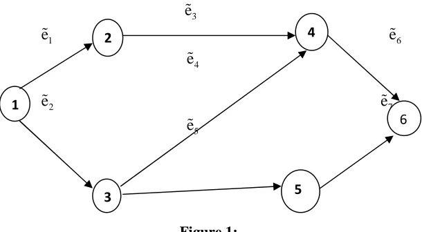
5. Numerical example

(6)

88

3

eɶ

1

eɶ

6

eɶ

4

eɶ

2

eɶ

7

eɶ

5

eɶ

Figure 1:

The edge weights are

1

eɶ = (0.5/0.8+0.4/0.7)/2 + (0.4/0.8)/3

2

eɶ _{= (0.3/0.8 + 0.8/0.7)/1 + (0.2/0.2)/3}

3

eɶ _{= (0.7/0.8)/2 + (0.9/0.6 +0.7/0.5)/4}

4

eɶ = (0.6/0.8)/4

5

eɶ _{= (0.9/0.6 +0.7/0.5)/3 + (0.4/0.3)/5}

6

eɶ _{= (0.8/0.7 + 0.4/0.5)/2}

7

eɶ eɶ7 = (0.6/0.6)/2 +(0.7/0.5+ 0.5/0.4)/4

Algorithm for finding shortest path length

Step 1: Form the possible paths from starting node to destination node and compute the

corresponding path lengths, Lɶ_i i = 1,2,. . . .n for possible n paths.

1

pɶ = eɶ₁+eɶ₃+eɶ₆= 1 – 2- 4- 6

2

pɶ = eɶ₂+eɶ₄+ eɶ₆=1 – 3- 4- 6

3

pɶ = eɶ₂+ eɶ₅ + eɶ₇=1 – 3- 5- 6

1

Lɶ = (0.5/0.7+0.4/0.5)/6+(0.4/0.7+0.4/0.5)/7+ (0.5 /0.6 +0.5/0.5)/8 + (0.4/0.6+0.4/0.5)/9

2

Lɶ = (0.6/0.7+0.4/0.5)/7 + (0.2/0.2)/9

3

Lɶ = (0.6/0.6 + 0.6/0.5)/6 + ( 0.2/0.5+0.2/0.4)/8 + (0.2/0.3)/10 + (0.2/0.2)/12

1

2

3

4

5

(7)

89

Step 2 :Find i

L

Cɶ using def 2.9

1 L

Cɶ = 0.04/7.3 + 0.04/7.4 + 0.04/7.5 + 0.032/7.6

2 L

Cɶ = 0.12/7.4 + 0.08/7.6

3 L

Cɶ = 0.0048/8.1 + 0.0048/8.3

Step 3 : Set

1

L L

Cɶ =Cɶ Step 4 : Let i=2

Step 5 : Compute C_Lɶ = Min (C_Lɶ, i

L

Cɶ ) using def 2.6.

C_Lɶ = 0.04/7.3 + 0.04/7.4 + 0.04/7.5 + 0.032/7.6

Step 6 : Set i = i + 1 Step 7 : If i≤ n goto step 5

Step 8 : The shortest path length is C_Lɶ

C_Lɶ = 0.0048/7.3 + 0.0048/7.4 + 0.0048/7.5 + 0.0048/7.6

Shortest path procedure

Step 1 : Compute the shortest path length is using shortest path length procedure

Step 2 : Let j = 1

j

L L

1 ( _L, _L)

d C Cɶ ɶ =0.0352

Step 4 : Compute ( , ) 1

1 ( , )

j

j L L

L L

s C C

d C C =

+

ɶ ɶ

1

1( L, L)

s C Cɶ ɶ =0.966

Step 5 : If j = 1, Assign ( , ) ( , )

j j j

L L L L

s C Cɶ ɶ =s C Cɶ ɶ

1 ( _L, _L)

s C Cɶ ɶ =0.966 Step 6 : Compute s = Max (S, Sj)

1 ( _L, _L)

s C Cɶ ɶ =0.966 Step 7 : Put j = j + 1

j = 2

Step 8 : If j≤n goto step 3.

2≤3 goto step 3

j

L L

2 ( _L, _L )

d C Cɶ ɶ = 0.1152

Step 4 : Compute ( , ) 1

1 ( , )

j

j L L

L L

s C C

d C C =

+

ɶ ɶ

(8)

90 2

2( L, L )

s C Cɶ ɶ =0.896

Step 5 : If j = 1, Assign ( , ) ( , )

j j j

L L L L

Here j = 2

Step 6 : Compute s = Max (S, Sj)

S = 0.966 Step 7 : Put j = j + 1

j = 3

Step 8 : If j≤n goto step 3.

3≤3 goto step 3

j

L L

3 ( _L, _L )

d C Cɶ ɶ = 0.0048

Step 4 : Compute ( , ) 1

1 ( , )

j

j L L

L L

s C C

d C C =

+

ɶ ɶ

3

3( L, L )

s C Cɶ ɶ =0.995

Step 5 : If j = 1, Assign ( , ) ( , )

j j j

L L L L

Here j = 3

Step 6 : Compute s = Max (S, Sj)

S = 0.995 Step 7 : Put j = j + 1

j = 4

Step 8 : If j≤n goto step 3. 3≤_{4 stop the procedure}

Step 9 : The Highest Similarity degree is S = 0.995 and that corresponding path

1 – 3 – 5 - 6is the Shortest path

and C_Lɶ = 0.0048/7.3 + 0.0048/7.4 + 0.0048/7.5 + 0.0048/7.6 is the

shortest path length.

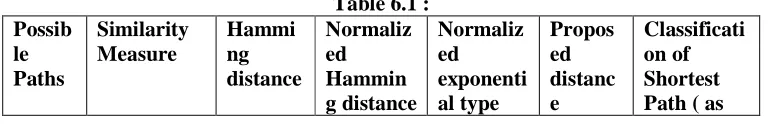
6. Results and discussion

In this section we have discussed our proposed distance and some existing distance measures. Our proposed system is make the calculation part as simplest one while comparing with other distances like Hamming, Normalized hamming etc., and we are getting the same shortest path in both proposed and some existing distance measures also. Here we have compared existing distance measures with our proposed distance measures. The highest similarity measure gives the shortest path from source node to destination node in the network.

Table 6.1 : Possib

le Paths

Similarity Measure

Hammi ng distance

Normaliz ed Hammin g distance

Normaliz ed exponenti al type

Propos ed distanc e

(9)

91

distance per

Similarity Measure)

1-2-4-6 s C C1( Lɶ, Lɶ1)=

0.883 0.9668 0.948 0.966 2

1-3-4-6 s C C2( Lɶ, Lɶ2)=

0.83 0.95 0.923 0.896 3

1-3-5-6 s C C3( Lɶ, Lɶ3)=

0.97 0.995 0.99 0.995 1

Hence the path P2 = 1 – 3 – 5 – 6 is having the highest similarity degree

2

2( L, L )

s C Cɶ ɶ =

0.995

7. Conclusion

The fuzzy shortest path problem in a network has been investigated in numerous articles because of its importance to various applications. It aims to offer a decision maker the shortest path length and the shortest path in a network with fuzzy arc lengths. For this purpose, in this paper, we proposed new approach to determine the shortest path length and the shortest path in a fuzzy network. Here type-2 fuzzy number has been reduced to type-1 fuzzy number using type reduction method.

REFERENCES

1. SK. Md. Abu Nayeem and M.Pal, Shortest path problem on a network with imprecise edge weight, Fuzzy Optimization and Decision Making, 4 (2005) 293 – 312.

2. V.Anusuya and R. Sathya, Type-2 fuzzy shortest path, International Journal of Fuzzy Mathematical Archive, 2 (2013) 36-42.

3. Avinash, J.Kamble and T.Venkatesh, Some results on fuzzy numbers, Annals of Pure and Applied Mathematics, 7(2) (2014) 90 – 97.

4. M.V. Dhanyamol and Sunil Mathew, Distances in weighted graphs, Annals of Pure and Applied Mathematics, 8(1) (2014) 1-9.

5. E.A.Jammeh, M.Fleury, C.Wagner, H.Hagras and M.Ghanbari, Interval type-2 fuzzy logic congestion control for video streaming across IP networks, IEEE Trans. Fuzzy Systems, 17 (2009) 1123 – 1142.

6. W.S.Kang and J.Choi, Domain density description for multiclass pattern classification with reduced computational load, J. Pattern Recognition, 141(6) (2008) 1997-2009.

7. N. Karnik and M. Mendel, Type-2 fuzzy logic systems: Type – reduction, in IEEE Syst., Man, Cybern. Conf., San Diego, CA, October 1998.

8. N. Karnik and M. Mendel, An introduction to type-2 fuzzy logic systems, USC Report, http://sipi.usc.edu/~mendel/report, oct. 1998.

(10)

92

10. N. Karnik and M. Mendel, Centroid of a type-2 fuzzy set, Information Sciences, 132 (2001) 195-220.

11. Lee Sang-Hyuk, Park Wook – Je, Jung Dong – Yean, Similarity measure design and similarity computation for discrete fuzzy data, J. Cent. South Univ. Technol., 18 (2011) 1602 – 1608.

12. J.M.Mendel, F.Liu and D.Zhai, α_{plane representation for type-2 fuzzy sets: theory}

and applications, IEEE Trans. Fuzzy Systems, 17 (2009) 1189 – 1207.

13. O.Mendoza, P.Melin and G.Licea, A hybrid approach for image recognition combining type-2 fuzzy logic, modular neural networks and the sugeno integral, Information Sciences, 179 (2009) 2078 – 2101.

14. M. Mizumoto and K. Tanaka, Some properties of fuzzy sets of type-2, Information and Control, 31 (1976) 312 – 340.

15. A. Nagoorgani, and V. Anusuya, Fuzzy shortest path by linear multiple objective programming, Proceedings of the International Conference On Mathematics and Computer Science,, Loyola College, Chennai, Jan 10 and 11, 2005, pp.287 – 294. 16. Y.Rebille, Decisin making over necessity measures through the choquet integral

criterion, Fuzzy Sets and Systems, 157 (23) (2006) 3025 – 3039.

17. F.Y. Shih, and K.Zhang, A distance-based separator representation for pattern classification, J. Image and Vision Computing, 26(5) (2008) 667-672.

18. C. Wagner and H. Hagras, Towards genera type-2 fuzzy logic systems based on zSlices, IEEE Trans. Fuzzy Systems, 18 (2010) 637 – 660.

19. R.R. Yager, Fuzzy subsets of type II in decisions, J.Cybern., 10 (1980) 137 – 159. 20. L.A. Zadeh, The concept of a linguistic variable and its application to approximate

reasoning – 1, Inform. Sci., 8 (1975) 199 – 249.

21. M.Pal and Hossein Rashmanlou, Irregular interval–valued fuzzy graphs, Annals of Pure and Applied Mathematics, 3(1) (2013) 56-66.

22. H.Rashmanlou and M.Pal, Isometry on interval-valued fuzzy graphs, Intern. J. Fuzzy Mathematical Archive, 3 (2013) 28-35.

23. H.Rashmanlou and M.Pal, Balanced interval-valued fuzzy graphs, Journal of Physical Sciences, 17 (2013) 43-57.