Chapter 6: GENERALISED LINEAR MODELS Yvonne M. Buckley
School of Natural Sciences, Trinity College Dublin, Dublin 2, Ireland. [email protected] The University of Queensland, School of Biological Sciences, Queensland 4072, Australia
6.1 Introduction
Ecologists in the past have often been taught individual statistical techniques in piece-‐meal fashion without the unifying conceptual model that lies behind them. This is changing rapidly and the increasing use of Generalized Linear Models is leading to a unification of modelling concepts in the minds of users. The beauty of generalized linear modelling is that it provides strong and stable “hooks” on which to hang additional knowledge, enables a re-‐interpretation of previously learned ANOVA and regression techniques and integrates well with more advanced modelling techniques introduced in chapters 12, 13 and 14.
Generalized Linear Modelling (GLM) unifies several statistical and modelling techniques. It is much easier to remember the structure and use of a GLM than to recall several disparate tests and rules to appropriately use ANOVA, ANCOVA, regression, multiple regression, logistic regression and logit regression. Any of these models, and more, can be described using an appropriate combination of just three properties of the GLM: the linear predictor, error distribution and link function which together enable the modelling of simple linear relationships with normal errors as well as more complex non-‐ linear relationships with alternative error distributions. To make life even easier the linear predictor is always linear, just like a standard regression, so we need only be concerned with variations in the error distribution and link functions used. The error distribution describes how the variation which is not explained as part of the linear predictor is distributed and the link function provides a link between the linear predictor and the response variable, as the response variable may not be directly linearly related to the explanatory variables in the linear predictor.
Classical linear models assume that errors, also called residuals or deviations from the fitted model, are normally distributed. This means that the errors take continuous values and are distributed according to the Normal or Gaussian probability distribution (see Appendix 6.A “normal data vs normal errors.r”). In a statistical modelling framework, the Normal distribution is the familiar bell-‐shaped curve with a high frequency of values close to zero (many small errors) and the frequency of larger positive or negative errors declining towards the tails of the distribution. The width or spread of the distribution is
determined by the variance of the errors. Because the Normal distribution of the errors around a fitted line has its mean at zero the only parameter of interest is the error variance around those fitted values. There is a very persistent myth that when we assess normality we are referring to the distribution of the original data. This is wrong. When we assess normality we do so with reference to the residuals or errors (see chapter 1, Fig. 6.1, Appendix 6.A “normal data vs normal errors.r”.
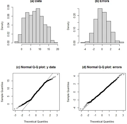
Fig. 6.1. The difference between assessing (a) normality of data (wrong!) and (b) normality of errors (right!) in linear modelling is shown here. These are histograms of simulated data drawn from a normal distribution with a specified relationship between x and y (intercept=0, slope=5) and a standard deviation of 1.5. As can be seen from the Normal quantile-‐quantile plots the original data are not necessarily normally distributed (c) but the errors are normally distributed (d) (errors=residuals from the fitted relationship). See the Appendix 6.A “normal data vs normal errors.r”.
[image:2.612.72.490.91.499.2]
In some cases the transformed data with Normal errors may lead to a better fitting, or simpler, model than a GLM (see Appendix 6.A “baccharis seeds.r” for an example using Normal, Poisson, Quasi-‐Poisson and Negative Binomial error structures). Model comparison and criticism will enable you to determine what the best course of action is in a particular circumstance.
Generalized Linear Models entered the ecological statisticians toolkit with the publication of McCullagh and Nelder’s landmark book in 1989 (McCullagh and Nelder 1989) and slowly gained in popularity among ecologists as statistical modelling programs were developed to implement GLM. GLM is now routinely taught to ecologists at undergraduate and graduate level. There are several texts that explain GLMs from different angles and with varying ecological, statistical and mathematical flavors (e.g. (Crawley 2007; Gelman and Hill 2007; Bolker 2008)) and I refer readers to these for complementary material. While students who have had experience with GLMs generally have a good grasp of the “how” to undertake a GLM analysis, in my experience they tend to lack an intuitive understanding of the model structure and properties of data that make some error distributions and link functions more appropriate than others. There is also confusion around how best to evaluate a GLM in terms of how appropriate it is for the data, how to plot data and models and what statistics to report. Here I aim to augment existing books, book chapters and papers on GLMs by focusing on the data/GLM interface.
Much of the data that ecologists commonly collect leads to the assumption of normality of errors being contravened. Count data such as number of species, number of cones on pine trees and number of offspring wolves produce are discrete, constrained to be positive, and may be clustered due to a biological process which is not directly modeled. Binary data (e.g. male/female, alive/dead) are discrete and bounded at 0 and 1, for example, a tree cannot be more dead than dead (0) or more alive than alive (1). Proportion data come in two main flavours: proportion data with a meaningful denominator, for example. the proportion of seeds in a known sample size which germinate or the proportion of frogs in a sample succumbing to chytrid fungus disease) and proportion data without a meaningful denominator, for example the % sand content of a soil sample or % cover of grass in a quadrat. Both types of
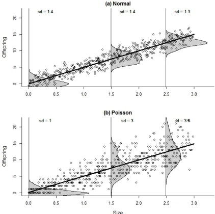
Fig. 6.2. Simulated data on offspring production of different sized individuals from a (a) Normal distribution) and (b) Poisson distribution (bottom). Note that simulating offspring production using normal errors leads to production of negative numbers of offspring as the normal distribution is not bounded at zero! The lines are fitted linear models assuming normal errors and the observed distribution of errors at three points is shown shaded grey ( a kernel density estimate was used). The errors in the top graph appear close to Normal in distribution (symmetrical bell shape) with a relatively constant distribution over the fitted mean values. The errors in the bottom graph may be skewed (particularly at low values) with regards to the Normal and with a variance that increases with the fitted mean values. See Appendix 6.A “normal and Poisson errors.r”.
[image:4.612.69.491.76.496.2]
determining statistical significance alone, to appropriately modelling a biological process it makes sense to use a model which captures more of the properties of the process we are trying to understand with our model. Often we are not only interested in the fitted relationship or mean response, but also the unexplained variation that surrounds the response. Variation in biological processes is commonly important, for example variation in population growth rate can influence extinction risk. Thus, it is necessary to describe the nature and magnitude of this variation appropriately, including how variation is distributed around the fitted values, as it may not be homogeneous. In addition, appropriate
modelling of error variance allows uncertainty in model outcomes to be accounted for.
GLMs are commonly used to parameterize population dynamics models as several of the vital rates determining population growth rate are best modeled using non-‐Normal error distributions (e.g. survival and number of offspring produced) (Merow, Dahlgren et al. 2014). Testing different model structures informs on the ecological process and knowing the ecological process informs the appropriate model structure (Coutts, Caplat et al. 2012). The resulting population models are used to make predictions about population growth rates or times to extinction. Scientists make recommendations for
management of pests or species of conservation concern based on statistical models of biological processes, therefore incorrectly modeled populations may lead to wasted management resources or adverse outcomes for the species concerned.
Proportion, binary and count data by their very nature tend to have fundamentally non-‐linear
relationships with explanatory variables. For example low numbers of seeds may be produced on a tree until a threshold tree size is achieved, leading to a log-‐linear relationship between seed production and size. Another example is that survival may be low at small sizes and high at large sizes leading to an S-‐ shaped, or logistic, relationship. GLMs enable the inclusion of inherent non-‐linearity through the link function. The link function relates the linear predictor, ηi which is not bounded and has homogeneous
variance, to the expected values of the data, which may be bounded and have heterogeneous variance. Link functions enable fitted values from the model of the linear predictor to be converted to non-‐linear predictions on the same scale that the data were collected; for example, in a GLM of survival data the appropriate link function (e.g. logit) enables fitting and predictions of probabilities bounded at 0 and 1.
Plot your data before starting the modelling process in order to determine what the likely relationships are and to explore the structure of variance in your data. While we should have mental models of what we expect our data to look like there are often surprises in store once it is collected. There is no
substitute for thorough knowledge of your data. Throughout the modelling process confront your models with data by looking at fitted relationships in contrast to your data. This is not always trivial, particularly for GLMs where data and fitted relationships can be plotted at the observed scale or at the scale of the linear predictor. Throughout the chapter I give several examples of plotting techniques and associated code.
6.2 Structure of a GLM
So, you suspect or know that you will require a GLM. Perhaps you have undertaken a classical linear model with normal errors and are unhappy with the standard diagnostic plots (heteroscedasticity of errors, non-‐linearity of the relationship, poor performance on a Q-‐Q normality plot – see Appendix 6.A “pine cones.r” for an example of what these might look like). Perhaps due to the nature of your data: count, proportion, binary or time to event, you suspect that a GLM would be appropriate. How do you choose an appropriate GLM structure? Let’s look first at the structural options for a GLM.
There are few exotic options here; the linear predictor is equivalent to a classical linear regression, ANOVA or ANCOVA model with one response variable and some combination of categorical and/or continuous explanatory variables as main effects and/or in interaction. Here your linear predictor ηi, for
each data point i, is a linear function of some explanatory variables (also called co-‐variates if they are continuous or factors if they are categorical) Xpi with an intercept, α, and slope or additional intercept
parameters, βp, corresponding to the 1 to p explanatory variables.
𝜂! =𝛼+𝛽!𝑋!!+⋯+𝛽!𝑋!" eqn. 6.1
Note that there is no error specified in the linear predictor, it just contains the systematic part of the model.
As with classical regression you can specify polynomial functions of continuous explanatory variables to deal with non-‐linear relationships; with polynomial models the linearity is retained in the parameters. To illustrate this: specifying a model as a+bx+cx2, to capture non-‐linearity in the response variable y in relation to variation in the x variable, is equivalent to calculating a new variable z=x2 and fitting a+bx+cz where y clearly has linear relationships with both x and z. For an example of fitting and testing a
quadratic term see Appendix 6.A “baccharis seeds.r”.
A useful extension of the classical linear model is the potential for specifying off-‐sets in the model. An off-‐set is an a priori value for a parameter in the model; you can then test the significance of the estimated difference between the given offset parameter and the freely estimated parameter. For example you might have a good reason to suspect that the slope of a relationship with a particular explanatory variable would take a particular value, e.g. slope=1. You set the value of that parameter in the model as an offset which means that instead of estimating the slope directly you get an estimate of the difference between a slope equal to the offset value and the estimated slope without the offset. You can then easily assess significance of the difference between the offset and the estimated parameter; this difference would be zero if the offset parameter and the estimated parameter were similar. See Appendix 6.A for an example using “pine cones.r”.
6.2.2 The error structure
Once an initial model for the linear predictor is constructed the next step is to decide on an appropriate error structure. There are good a priori reasons for choosing particular error distributions for particular types of data. The first distinction is between continuous and discrete error distributions. If your response variable contains continuous data (e.g. size, weight, and gene expression) you will need a continuous error distribution. The most familiar distribution in this class is the Normal or Gaussian error distribution which has two parameters, the mean and the variance.
For a Normal error distribution the error distribution model would be:
𝐘~𝑁(𝛍,𝜎!) eqn. 6.2
Predictions of the vector of Y values are estimated to come from a Normal distribution with a mean µ and a constant variance σ2, hence N(µ, σ2) . The mean, µ, is a vector of fitted values describing the relationship between the response variable and the explanatory variables. The value of the vector µ therefore changes depending on which values of the explanatory variables you look at. There is just one value for the variance σ2 which does not change depending on the fitted values. For the case of the Normal distribution the link function between the linear predictor and the predicted values is the identity link which means η=μ. Other error structures are presented in section 6.3 below.
The final part of a GLM structure is the link function, this important element links the linear predictor (linear model whose fitted values can take any negative or positive value) to the original response variable via a function. Where we use Normal errors the link function is the identity link which means the linear predictor automatically predicts on the scale of the original response variable. For counts however the fitted values should only take values greater than zero, so we need a function that maps the linear predictor (any value) to only positive values.
In the case of the normal distribution of errors the appropriate link function which connects the linear predictor with the mean of the normal distribution is the identity link, η=µ. In general, η=g(µ), with g() called the link function. Usually we have the linear predictor η (fitted values on the scale of the linear predictor) and we want to convert these to the predicted means µ (equivalent to the fitted values on the scale of the response variable Y). To do this we apply the inverse of the link function g()-‐1 and for the normal error case the inverse of the identity link is still the identity link η=µ and µ =η. The expectation of the response variable Y is therefore equivalent to the fitted values at both the linear predictor and response scales, E(Y)= µ=η. Other link functions are presented table 6.1.
A particular value of the response variable Yi is modeled using a Normal distribution with mean coming
from the linear predictor, 𝜂!, and error variance 𝜎! with a random number from that error variance
given by 𝜀! . 𝑌! =𝜂!+𝜀! , note that negative fitted values could be predicted if ηi is predicted to be
negative for some values of the explanatory variables, or if negative errors reduce Yi sufficiently. This is
important to note when modelling a process that inherently is bounded at zero, negative values may make no biological sense for variables such as size (-‐Chapter 5). The full model including the linear predictor, error distribution and link function is therefore:
𝐘~𝑁(𝑔(𝜼) !!,𝜎!) eqn. 6.3
6.3 Which error distribution and link function are suitable for my data?
In general GLMs allow for the error distribution to come from an exponential family other than the Normal and the link function may be any monotonic differentiable function (continuously increasing or decreasing function with a gradient calculable using differentiation). Canonical links are specified for each family of error distributions which are statistically convenient but are not necessarily always the best fit, in which case alternative link functions can be used.
How do we choose an appropriate link function? The canonical link function is a good starting point. See table 1 for a list of error distributions and associated link functions. However, there may be several different link functions which could be applied to your model and it makes sense to try a few and compare model fits to determine the most appropriate link. In R you can get a list of potential links for each distribution by typing ?family.
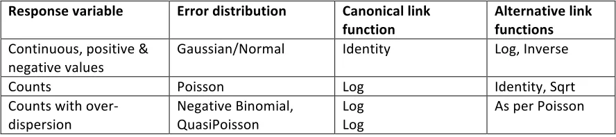
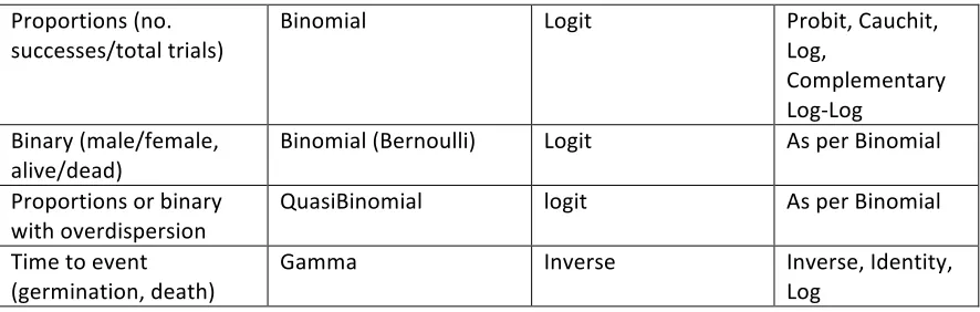
Table 6.1. Appropriate error distributions, canonical link functions and alternative link functions for commonly modeled response variables (for details on distribution properties see Appendix A).
Response variable Error distribution Canonical link function
Alternative link functions Continuous, positive &
negative values
Gaussian/Normal Identity Log, Inverse
Counts Poisson Log Identity, Sqrt
Counts with over-‐ dispersion
Negative Binomial, QuasiPoisson
Log Log
[image:7.612.102.546.622.721.2]Proportions (no.
successes/total trials) Binomial Logit Probit, Cauchit, Log, Complementary Log-‐Log
Binary (male/female,
alive/dead) Binomial (Bernoulli) Logit As per Binomial Proportions or binary
with overdispersion QuasiBinomial logit As per Binomial Time to event
(germination, death) Gamma Inverse Inverse, Identity, Log
The Gamma, Beta, Exponential and LogNormal distributions are alternative continuous error
distributions that are used for different kinds of continuous response variables. For example the Beta distribution can be useful for modelling proportion data that is not from success/failure trials, such as percent cover data for plant community assessment. The Gamma distribution is useful for “time to failure” data such as time to germination or time to death (Chapter 5). See chapter 3, Appendix A and (Bolker 2008) for a discussion of distributions and their properties.
If your response variable contains discrete data you will need to use a discrete probability distribution function. Discrete response variables include: counts (which are constrained to be greater than zero and constrained to integer values), binary events (such as success/failure, survived/died, male/female) and proportion data which were collected as number of successes from a series of trials. The most
commonly employed error distributions for ecological data include the Binomial for binary and
proportion data and the Poisson for count data. Below I give two examples for ecological data which are appropriately analyzed using the Binomial error distribution and the Poisson error distribution
respectively. I have also provided worked examples of Binomial (“tree death.r”) and Poisson, quasi-‐ Poisson and Negative Binomial (“baccharis seeds.r”, “pine cones.r”) models in Appendix 6.A.
6.3.1 Binomial distribution
The probability of success in any trial is p, for example the probability of a tossed coin landing heads up (a “success”) is 0.5, p=0.5. You might undertake a number of trials, n, resulting in a number of successes, k. We can use the Binomial distribution to estimate, for example, the probabilities of getting 4 heads (k=4) in a series of 5 trials (n=5).
Pr (X=k)= !! 𝑝!(1−𝑝)!!! eqn. 6.4 For k=0,1,2,…,n
[image:8.612.103.546.70.211.2]
Fig. 6.3. Variance from a Binomial distribution with number of trials n=5 or the special case of the Bernoulli distribution where n=1. Variance is at its lowest (0) at probability of survival=0 where all individuals die and probability of survival =1 where all individuals live and is at its maximum at probability of survival=0.5 where survival and mortality are both equally likely. See Appendix 6.A “binomial.r”.
Trees are generally long lived and tree death is difficult to observe without long term repeated
measures. However, we can take advantage of mass mortality events, such as during droughts, to look at individual vulnerability to mortality. Data were collected on tree mortality, a binary variable, as well as tree size (diameter at breast height) and other potential influences of mortality such as neighborhood density and location. Here I use this example to analyses the effects of tree size and location on
determining vulnerability to mortality during a drought episode, for further analyses of these data see (Dwyer, Fensham et al. 2010).
Survival is a binary variable, taking only two values, alive or dead. The errors may therefore be distributed according to the Bernoulli distribution which is a special case of the Binomial distribution with just one trial. Thus each tree can be viewed as a trial with a possible outcome of alive or dead. As tree size increases we would expect survival to increase as adults are more deeply rooted, potentially accessing water reserves unavailable to seedlings. At small sizes perhaps most trees die so variance in mortality is again low. Somewhere in the middle trees might be equally likely to die or survive leading to high variance at intermediate sizes. In this situation variance is obviously not homogeneous across the range of the explanatory variable (size), and is likely to be distributed according to the
Binomial/Bernoulli distribution around the mean with the variance of the distribution changing with the mean, see Fig. 6.3.
Binary data can be difficult to visualize in relation to explanatory variables. For the survival example binary alive or dead is the response variable (see Fig. 4) with a continuous tree diameter as the
[image:9.612.75.337.113.330.2]simple plot of the binary variable can mask the density of points as points are overlaid on each other. Introducing a jitter, a random displacement of small magnitude to the binary points, enables better visualization of the density of points along the x axis. A more intuitive understanding of the relationship with the explanatory variable can be gained by “binning” binary values along intervals and taking the means for each interval along the x-‐axis. This can be done by taking the mean of the binary points at even spacing along the x-‐axis or by creating bins with equal numbers of observations. However the patterns observed vary depending on the intervals used for finding the means (Fig. 4).
Fig. 6.4. Four ways of plotting a binary variable against a continuous explanatory variable. Observations (a) were of trees that were either alive (1) or dead (0). Observations with jitter (b) are the observations of 0’s and 1’s with a small uniformly distributed random variable added to separate the points vertically to enable better visualization of point density along the x-‐axis. The average of the evenly spaced observations (c) was found by taking the means of survival in 11 x 5 cm diameter categories. The average (Av.) of the equal number of observations (d) was found by taking the means of survival in 11 categories with approx. the same number of observations in each (n=40), these data were taken from site 1 of the Eucalyptus melanophloia survival data set (Appendix 6.A “tree death.r”).
The linear predictor is given by:
[image:10.612.67.441.187.551.2]Where X1 is tree diameter and α and β are the intercept and slope respectively. The linear predictor 𝜼 is a Real number and can be positive or negative depending on the values of the parameters and the explanatory variable. However, survival can only lie between 0 and 1 so we need relationship between survival and the linear predictor that is bounded at 0 and 1. The logit link function can achieve this:
𝛈=logit 𝒑 =log 𝒑
!!𝒑 eqn. 6.6 The inverse link function used to re-‐scale the linear predictor back to the 0-‐1 probability scale is:
𝒑=logit!! 𝜼 = !"# (𝜼)
!"#𝜼!! eqn. 6.7 and the full error model for using the Binomial (B) error distribution is:
𝐘~𝐵 𝐧,𝐩 eqn. 6.8 where n is the number of trials (in the Bernoulli case n=1 but in the general Binomial case n can be a vector of trials with, potentially, a different number of trials for each data point)and p is the inverse logit of the linear predictor as in eqn. 6.7.
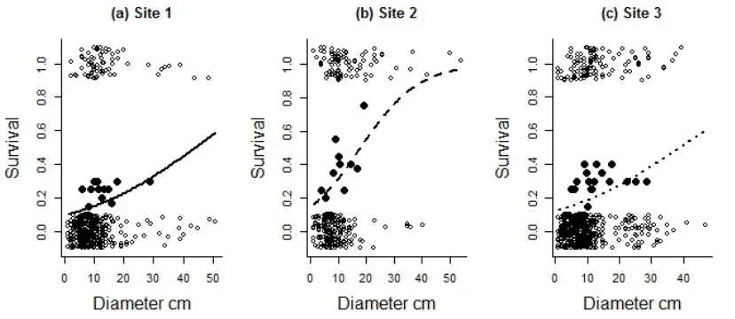
I like to explore and present my data as close to how it was collected as possible so would prefer to see the original data points if possible on figures. Fig. 6.5 attempts to reconcile this preference with showing the fit of the data to the model (it shows a combination of fig 6. 4. panels (b) and (d) with fitted lines from a GLM for three sites).
Fig. 6.5. Survival of Eucalyptus melanophloia trees of different diameters from three sites. The unfilled circles are the observed values (0 and 1 values with a vertical jitter added to aid visualization), the filled circles are averages of survival in 11 categories with approximately equal numbers of observations in each category (n=20) and the line represents the predicted probabilities from a GLM with Binomial errors and a logit link function. The predictions are not straight lines and are bounded at 0 and 1 as they have been re-‐scaled from the linear predictor to the survival probability scale using the inverse link function.(see Appendix 6.A “tree death.r”).
[image:11.612.69.483.325.505.2]
“binomial.r” . This is important even in a well-‐designed experiment with an equal number of trials across all sampling events as organisms can die, petri dishes can fall off benches and infections can compromise cultures resulting in uneven numbers of trials and variation in the denominator of your proportion. Always monitor and collect the sample size of a series of trials which make up your proportion data. You model proportion data in a GLM as a two-‐column response variable of (success, failure) where the number of failures is calculated as number of trials-‐number of successes. Use the cbind() function in R to combine the (success, failure) data and treat it like a single response variable. See appendix 6.A “binomial.r” for an example of a proportion calculated as the mean of eight individual proportions ignoring the denominator, contrasted with a proportion calculated using the binomial denominator which weights estimates towards the larger denominators.
6.3.2 Poisson distribution:
Count data have a number of properties which we need to account for in models: many zeros, bounded at zero, non-‐linearity and non-‐homogeneity of variance. The occurrence of many zeros may call for zero-‐ inflated error distribution methods (Ch. 12) (see Appendix 6.A for a discussion of zeros in the pine cone example ‘pine cones.r’). Because data are bounded at zero, the relationship with covariates (e.g. tree age, year and pine tree density) is often non-‐linear and the variance often increases with the mean (see Fig. 6.2). A pervasive recommendation, to normalize errors and linearize the relationship with
covariates, is to log-‐transform the response variable and use classical regression methods with Normal errors. However, this is potentially problematic for a number of reasons, the most serious of which in my view is the addition of an arbitrary amount (usually 1 or smaller) to the response, because zeros cannot be logged. See (O’Hara and Kotze 2010) for a thorough discussion of this issue from an ecological viewpoint. The use of a GLM may solve these problems; by modelling errors using alternative
distributions it may be possible to find a distribution that adequately captures the increase in variance with the mean and an appropriate link function can linearize the relationship for the linear predictor.
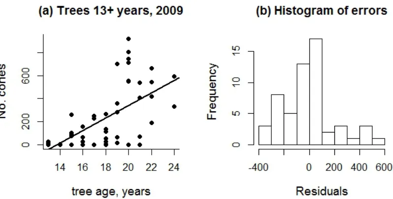
Pine cones contain seeds which determine the reproductive output of individuals and the population. The number of cones on trees is a discrete count variable, bounded at zero. A simple linear model of how tree size predicts number of cones with Normal errors is inappropriate for a number of reasons including that the counts are discrete and bounded at zero (Fig. 6.6).
[image:12.612.78.477.503.705.2]
Fig.6.6 The number of cones on individual pine trees of different ages (a) demonstrates several common issues with count data: many zeros which inflate residual variance, bounding at zero which decreases negative residual variance at low fitted values, non-‐linearity of the response to the explanatory variable and variance which increases with the explanatory variable. The line in (a) is an inappropriate linear model fitted to the data. The distribution of errors resulting from the linear fit is obviously not Normal (b) (see Appendix 6.A “pine cones.r”). Data from (Caplat, Nathan et al. 2012; Coutts, Caplat et al. 2012).
There is only one parameter in the Poisson (P) distribution, the mean μi, and the variance is assumed to
increase in direct proportion to the mean with a dispersion parameter of 1 (Fig.6. 3).
𝐘~P(𝝁) eqn. 6.9 The response variable Y is therefore Poisson (P) distributed with mean µ and variance µ, where µ is determined by the linear predictor and link function of the values of the explanatory variables in the model. If errors are Poisson distributed the fitted values on the original count scale will have an
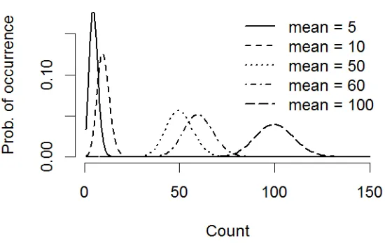
increasing spread of errors around them as µ increases. At large count means, and if the range of values you are modelling is not large relative to the mean, a Normal error distribution may be an adequate approximation, particularly in combination with a log transformation of the response (Fig. 7).
Fig. 6.7. Probability distribution function for the Poisson distribution with means of 5, 10, 50, 60 and 100 counts. The variance or errors increase as the mean increases, however, at large mean counts the distribution becomes symmetrical and a normal distribution may be a reasonable approximation (Appendix 6.A “poisson.r”).
A commonly used link function for Poisson models of count data is the log link, 𝜼=log 𝝁 with the inverse link as exp (𝜼)=𝝁 to convert the fitted values from the linear predictor back to positive values which can be directly compared with the observed count data.
[image:13.612.75.350.338.512.2]
offspring produced if you do reproduce, number of individuals observed if detected) as a Poisson model of counts. You could also simultaneously model both processes in a mixture model (chapter 12). If zero counts arise as a separate process from other counts then consider collecting data on additional explanatory variables which could be determinants of zeros as these data will greatly improve the resulting two-‐stage or mixture model (e.g. organism age or maturity or characteristics of observer, see appendix 6.A “pine cones.r”).
6.3.3 Overdispersion
Overdispersion is a relatively common problem encountered when using Poisson and Binomial error distributions. There is assumed to be a strong (for Poisson, exact) relationship between the mean and the variance in both distributions. Quite often with biological data there is more variance in the errors than can be explained by the Binomial or Poisson distribution, see chapter 12 for a thorough treatment of overdispersion. This can be assessed by dividing the residual deviance (of the GLM model) by the residual degrees of freedom, if this quotient is substantially greater than unity (1) then overdispersion is a problem (for examples of over-‐dispersion see Appendix 6.A “baccharis seeds.r”, “pine cones.r”). It is difficult to give a threshold at which overdispersion becomes “substantial”. Minor overdispersion can be dealt with if the underlying process can be adequately modelled with a known distribution such as the Binomial or Poisson. You should explore the consequences of overdispersion for your model inference and use that as a guide to whether it is problematic or not. For example you could take some of the steps suggested below and see if they change your conclusions. More serious overdispersion may be a result of a miss-‐specified model.
There are some quick and dirty fixes for mild overdispersion including switching from using Chi-‐squared to more conservative F-‐tests to assess significance and the use of quasi distributions. Which methods you should use depend largely on the purpose of your model, if you are looking to assess significance of explanatory variables alone and are not interested in parameter estimates then switching to F-‐tests might suffice. However, this is not a philosophy I am particularly comfortable with as I prefer to model to get insight into process rather than just model for significance tests. Quasi methods do not use a specified error distribution, rather they estimate an additional parameter to relate the mean and the variance, but still based on either the Binomial or Poisson distributions, hence quasi-‐Poisson or quasi-‐ Binomial. Quasi methods are therefore not necessarily self-‐contained error distributions which capture characteristic behaviour of a process, they can be viewed as “hacks” of underlying distributions. If your errors are really not a result of Binomial or Poisson processes then quasi-‐B or quasi-‐P models are also not appropriate. They should only be used to account for mild overdispersion as a result of minor deviation from the assumptions of Binomial or Poisson distributions. The additional parameter in a quasi model is named the overdispersion or scale parameter. Quasi models are parameterized using quasi-‐ likelihood methods (Chapter 3). You will notice that if you compare a quasi-‐model with a specified distribution model (Poisson or Binomial), the standard errors of the parameter estimates become larger using the quasi model (ref to the appendices), therefore you can easily come across situations where the use of the Poisson or Binomial family can lead to conclusions of significance but accounting for
overdispersion using a quasi-‐model can change those conclusions. It is therefore very important to be aware of overdispersion and to know how to deal with it.
If you have serious overdispersion you may be miss-‐specifying your model and rather than switching immediately to quasi approaches it may be more appropriate to consider alternative model
constructions and error distributions. For count data a negative binomial error distribution can
seems to fit better at low tree ages, better capturing low numbers of cones produced (Appendix 6.A “pine cones.r”). Another alternative is to use mixed effects models and include a random effect at the level of the observations (chapter 13). Generalized mixed effects models have improved considerably in computational tractability making them a useful alternative to quasi approaches.
Zeros can arise due to underlying environmental heterogeneity or individual differences in quality which cannot be readily observed, causing overdispersion. Overdispersion can arise from unknown or
unmodelled sources of variation which cause heterogeneity in the response variable at different scales. Overdispersion may be eliminated or substantially reduced by collecting the right covariates. Consider collecting spatial co-‐ordinates/locations or individual identities and using these as random effects within mixed effects models, inclusion of random effects at the individual level can be very effective at dealing with over-‐dispersion(Chapters 10 and 13), also see chapter 12 for the use of mixture models to deal with overdispersion.
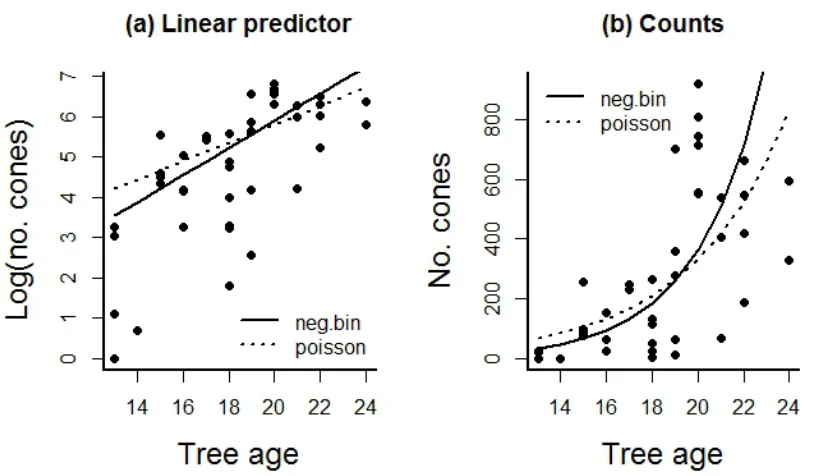
Fig. 6.8. Here we compare (a) the fit of the linear predictor when using Poisson and Negative Binomial error distributions and (b) the same models and data plotted on the original count scale. This figure illustrates that the error distribution you choose affects the parameter estimates and also demonstrates the difference between the fitted values from the linear predictor and the fitted values from the linear predictor with the inverse link function applied to convert them back to the count scale (see Appendix 6.A “pine cones.r”).
6.4 Model fit and inference
[image:15.612.70.477.274.512.2]function of a quasi-‐model collapses down to the Poisson or Binomial when the scale parameter is set to one, hence quasi-‐Poisson or quasi-‐Binomial.
Often we would like to know whether our experimental treatment or co-‐variate makes a “significant” difference to our observations, i.e. whether the differences observed between treatments are likely to have arisen by chance or not. An appropriate statistical model will adequately model the “by chance” component of this, i.e. the error distribution. Without an appropriate model of the errors we risk finding false significance or not finding significance when we should (type I and II errors, chapter 2).
Model fit for GLMs is assessed using deviance. The (residual) deviance D is the GLM equivalent of the residual sum of squares. Technically, it is the difference between the log-‐likelihood of the saturated model, where the saturated model has as many parameters as observations, and the log-‐likelihood for the fitted model:
𝐷=−2(log 𝑝 𝑦𝜃! −log 𝑝 𝑦 𝜃! ) eqn. 6.10
Where 𝜃!are the fitted values of the parameters in the fitted model and 𝜃! are the parameters in the
saturated or full model, y represents the observed response data. Deviance is therefore the difference between the logs of the probability of the data given the fitted values 𝑝 𝑦 𝜃! and the probability of the data given a fully saturated model 𝑝 𝑦𝜃! , multiplied by -‐2. The probability of the data in the saturated model will be large (i.e. close to 1!) because you are explaining all the variance in the data by using as many parameters as there are data points. Log(1)=0 and the log of probabilities lower than 1 are negative so the difference between the two log terms will be negative and the absolute value will be larger if the fitted model is not very good. The higher the deviance therefore the worse the fitted model is. As in life, in statistics higher deviance is bad news.
Chapter 3 presents a thorough treatment of model selection processes, I provide a brief summary with some GLM specific issues below. If your fitted model is a good description of the data you would expect a small deviance from the saturated model, if the deviance is small you would accept the simpler model (all models which are nested within the saturated model will be simpler!). Operationally we are
interested in whether one model which is a simplification of a more complicated model is better. In this case we can use deviance to compare the likelihoods of the more complex model and the nested
simpler one (Chapter 3). We use a Chi-‐squared (Χ2) distribution to assess whether the resulting deviance is small or large. We therefore compare the difference in deviance between the two models to a Chi-‐sq. distribution with p1-‐p2 parameters, which is the difference between the number of parameters in the two models. A low P value indicates that the deviance is large and that the models are different, we would infer that you lose important information using the simpler model and may therefore choose to retain the more complex model. A high P value indicates that the deviance is small, there is little difference in explanatory power between the two models and we would therefore choose the simpler model. We report the LRdf or Χ2df as our test statistic and its associated P value.
different kind of deviance test is used: !!!!!
!!!! ~𝐹 where the test statistic is assumed to follow the F distribution rather than the Chi-‐sq distribution. ρ is the dispersion parameter and p+1 and q+1 are the number of parameters in models 1 and 2 respectively. D1 is the deviance of the more complex model
and D2 of the simpler nested model. The LR test statistic follows an F-‐distribution with p-‐q and n-‐p degrees of freedom so we report LRp-‐q, n-‐p or Fp-‐q, n-‐p and its resulting P-‐value.
As GLMs with specified error distributions have an associated log-‐likelihood an Akaike information criterion (AIC) can be calculated and multi-‐model inference using information criteria can be carried out easily. Quasi models have a quasi-‐likelihood and quasi Akaike information criterion (QAIC) can be used for inference. Methods exist and can be used to extract QAIC from these models but note that R does not give you QAIC as part of the model summary automatically. See (Richards 2008) for a discussion and ecological examples of the use of QAIC for model selection.
6.5 Computational methods and convergence
Sometimes, despite our best efforts models can fail. Models can fail in a number of different ways; one of the most common is non-‐convergence. The default method for fitting GLMs in R is iteratively
reweighted least squares (IWLS). This algorithm uses the maximum likelihood function to determine iteratively “better” estimates of the parameters, ideally converging on a set of parameter estimates where the likelihood of the data is maximized. A model is determined to have converged when
successive iterations of the algorithm no longer improve the fit, or improve it only a very small amount. The shape of the likelihood surface determines how quickly and how well this process of convergence happens. If the likelihood surface is very flat, i.e. the data are relatively equally likely to occur under a large number of combinations of parameter values, there can be difficulty with convergence.
Non-‐convergence can happen for a number of reasons:
• your original mental model of the process may be wrong, perhaps you are using non-‐informative explanatory variables
• the process is inherently non-‐linear and you have not appropriately modelled the non-‐linearity • insufficient data were collected
• use of an incorrect likelihood function (i.e. the wrong error distribution),and/or link function See Appendix 6.A “pine cones.r” for an example of non-‐convergence when modelling data with lots of zeros using a negative binomial error distribution. In this case an appropriate single distribution could not be found so alternative models such as mixture models should be explored (see chapter 12).
may be because that variable truly is a great predictor or it may be that you have too few data points for a particular variable or combination of variables. If it is a sampling problem then you should increase your sample size, or try a different (probably simpler) model.
Warning messages about non-‐convergence should not be ignored; instead you should investigate the reason/s for non-‐convergence and be aware that the parameter estimates reported from a non-‐ converged model may be nonsense. If you can’t find a structural problem with your data or model causing the non-‐convergence then you can try to increase the number of iterations and/or specify some appropriate starting values. You should consider specifying starting values if you are using a quasi-‐model or an unusual combination of error distribution and link function.
6.6 Discussion
GLMs free us to collect more biologically meaningful data as we are not constrained to collection of just continuous response variables or response variables which can be readily transformed to meet the assumptions of linear models. There are, however, limits to what GLMs can do. Moving from classical linear models to GLMs means the replacement of assumptions of linearity and normality of errors with alternative assumptions about linearity and alternative error distributions. These new assumptions may not be appropriate. Errors from count data may not be Poisson distributed if the variance increases more rapidly than the mean (overdispersion) or there is clustering in the data. Errors from binary or proportion data may not be Binomial if there is overdispersion in the data. Models may not converge. The assumptions and predictions of GLMs need to be just as carefully investigated as the assumptions of linearity and normality in classical linear models.
Despite these limits GLMs are foundational units of many more complex modelling techniques. The skills and knowledge you attain by fitting and critiquing GLMs will pay dividends when learning more complex modelling techniques. It is important to note that real world data are messy; sometimes, despite a well-‐ designed experiment and careful data collection, the assumptions of GLMs just cannot be met. Perhaps an appropriate error distribution cannot be found, the models all fit poorly or models do not converge. There are many alternative ways of modelling data including (but not restricted to): non-‐linear models, non-‐parametric methods (particularly useful for error distributions which do not conform to common distributional assumptions), mixture models (chapter 12) and mixed effects models (chapter 13). If you think something biologically interesting is going on with your data-‐set you may want to invest in reading about and learning appropriate alternative techniques, starting with those in this book and moving beyond.
It’s the ecology, stupid! We pay attention to these statistical issues so we can have some confidence in the answers we get. With our models we look for insight into the ecological processes producing the patterns around us. The right error distribution and link function are not just statistical rules to be followed blindly. Informed and appropriate modelling of errors and link functions can enable more general predictions to be made as we strive to capture the ecological processes important to the generation of observed patterns.
Symbol Meaning
η linear predictor
α intercept
β slope
σ2 variance
ε Error
p probability
𝐷 Deviance
𝜃! fitted values of the parameters in the fitted model
𝜃! parameters in the saturated or full model
LR likelihood ratio
Χ2 Chi-‐square value
F F statistic value
ρ dispersion parameter
References
Bolker, B. M. (2008). Ecological models and data in R. Princeton, New Jersey, USA, Princeton University Press.
Caplat, P., R. Nathan, et al. (2012). "Seed terminal velocity, wind turbulence, and demography drive the spread of an invasive tree in an analytical model." Ecology 93(2): 368-‐377.
Coutts, S. R., P. Caplat, et al. (2012). "Reproductive ecology of Pinus nigra in an invasive population: individual-‐ and population-‐level variation in seed production and timing of seed release." Annals of Forest Science 69(4): 467-‐476.
Crawley, M. J. (2007). The R book. Chichester, UK, John Wiley & Sons Ltd: 942.
Dwyer, J., R. Fensham, et al. (2010). "Neighbourhood effects influence drought-‐induced mortality of savanna trees in Australia." Journal of Vegetation Science 21(3): 573-‐585.
Gelman, A. and J. Hill (2007). Data analysis using regression and multilevel/hierarchical models. New York, Cambridge University Press.
McCullagh, P. and J. A. Nelder (1989). Generalized Linear Models. London, Chapman & Hall.
Merow, C., J. P. Dahlgren, et al. (2014). "Advancing population ecology with integral projection models: a practical guide." Methods in Ecology and Evolution 5(2): 99-‐110.
O’Hara, R. B. and D. J. Kotze (2010). "Do not log-‐transform count data." Methods in Ecology and Evolution 1(2): 118-‐122.
Richards, S. A. (2008). "Dealing with overdispersed count data in applied ecology." Journal of Applied Ecology 45: 218-‐227.
Venables, W. N. and B. D. Ripley (2002). Modern Applied Statistics with S, Springer.
Warton, D. I. and F. K. C. Hui (2010). "The arcsine is asinine: the analysis of proportions in ecology." Ecology 92(1): 3-‐10.