Noname manuscript No. (will be inserted by the editor)
Long Memory and Changepoint Models: A Spectral
Classification Procedure
Ben Norwood · Rebecca Killick
Received: date / Accepted: date
Abstract Time series within fields such as Fi-nance and Economics are often modelled using long memory processes. Alternative studies on the same data can suggest that series may actu-ally contain a ‘changepoint’ (a point within the time series where the data generating process has changed). These models have been shown to have elements of similarity, such as within their spectrum. Without prior knowledge this leads to an ambiguity between these two mod-els, meaning it is difficult to assess which model is most appropriate. We demonstrate that con-sidering this problem in a time varying environ-ment using the time varying spectrum removes this ambiguity. Using the wavelet spectrum we then use a classification approach to determine the most appropriate model (long memory or changepoint). Simulation results are presented across a number of models followed by an ap-plication to stock cross correlations and US in-flation. The results indicate that the proposed classification outperforms an existing hypothe-sis testing approach on a number of models and performs comparatively across others.
Keywords Classification · Long Memory · Changepoint·Wavelet Spectrum· Nonstation-arity
Ben Norwood
Department of Mathematics & Statistics, Lancaster University, LA1 4YF, UK E-mail: [email protected]
Rebecca Killick
Department of Mathematics & Statistics, Lancaster University, LA1 4YF, UK Tel.: +44-1524-593780
E-mail: [email protected]
1 Introduction
It is not often the case that a given data set has a known explicit model from which it is generated. Analysts will look to fit an appro-priate model to such a series in the hopes of understanding the underlying mechanisms or to make predictions into the future. The models proposed are expected to be distinct in their properties such that there is a clear prevalence of a suitable model for the data. However, mod-els with certain structural features have been known to have similar properties to other mod-els [11]. This overlap will be here referred to as an ‘ambiguity’ between the models. This is such that either model may appear similar to one another in some metrics, but provide very different interpretations on the data generating process, and lead to different predictions into the future.
In this paper we consider the ambiguity be-tween long memory and changepoint models. This ambiguity has been documented in fields such as Finance and Economics which are mod-elled using long memory models [10, 26] and changepoint models [19, 28]. Thus it is reason-able to assert that there is an element of ambi-guity between these two models. Following the discussion and in-depth analysis within [6], it has been shown that both models share some similar properties, especially within the spec-trum. Often a decision on a model can not be made with the ‘luxury’ of prior knowledge, and as such assuming the data derives from either of these models comes at a risk of mis-specification.
the justification that this is the more plausi-ble model. However in some circumstances this may not be the case so it leads to the question as to which model should be the null model. It would be entirely feasible to choose the change-point model as the null model, not reject H0 and then flip to have the long memory model as the null model and also not rejectH0. This does not give a clear answer to the question of an appropriate model.
As an alternative this paper introduces a classifier, which places no such assumptions on which model is preferred. Instead the purpose of a classifier is only to give a measure of which category provides the best fit. In the context here, it can measure which model best describes a time series, without assuming that this model is where the data was originally generated from. Classification of time series has been previously used in [9] and [18]. It was shown in [30] that the autocorrelation function and periodogram of data generated from a changepoint model and a long memory model exhibit similar struc-tures (i.e. slow decay in the autocorrelation and spectral pole at zero). However, if we consider a time-varying periodogram, then the station-arity of a long memory model can be seen (con-stant structure over time), whilst a changepoint model exhibits the piecewise stationarity ex-pected (see for example [16]). As the time vary-ing spectrum shows evidence of a difference be-tween these models, we use it as the basis for our classification procedure.
The structure of this article is as follows. The background and methods to our approach are given in detail in Section 2. A simulation study of the proposed classification method, with a comparison to the Likelihood Ratio Test from [30], can be found in Section 3. Applications of the classifier are then given using US price in-flation and stock cross-correlations in Section 4. Finally, concluding remarks and a discussion is given in Section 5.
2 Methods
2.1 Changepoint and Long Memory Models
The aim of our method is to distinguish be-tween data which arises from either a change-point or a long memory model. To define these, we first define the general Autoregressive Inte-grated Moving Average (ARIMA) model, char-acterised by its Autoregressive (AR) parame-tersφ∈Rp, Moving Average (MA) parameters θ∈Rqand the Integration (I) parameterd∈N.
For random variablesX1, X2, . . . , Xnthis is for-mally defined as,
1− p X
k=1
φkBk !
(1−B)dXt= 1 + q X
k=1
θkBk !
t
wheret∼N(0, σ2) andBis the backward shift operator such that BXt = Xt−1 and Bt =
t−1. A variation of this, Autoregressive Frac-tional Integrated Moving Average (ARFIMA) is such that d∈R, allowing it to be fractional. This modification allows long memory behaviour to be captured through dependence over a large number of previous observations.
For the purpose of this paper, we define the changepoint and long memory models as:
Xt∼ (
µ1+ ARMA(φ1,θ1) if t= 1,2, . . . τ
µ2+ ARMA(φ2,θ2) if t=τ+ 1, τ+ 2, . . . n.
(1)
Xt∼µ+ ARFIMA(φ, d,θ) t= 1,2, . . . , n(2) Note that we depict a single changepoint τ = bnλc for notational ease, but the software we provide (see Section 5) contains the generali-sation to multiple changes through use of the PELT algorithm [17] and extending Equation (1) to include multipleτ. Other models such as ARCH models and Fractional Gaussian Noise [21] could also be used but we restrict our con-sideration to ARFIMA here. In the general case we allow p, q ∈ N, but in the simulations and applications given in Section 3 and 4 we restrict their range for computational reasons.
2.2 Wavelet Spectrum
The ambiguity present between diagnostics of the competing models given in Equation (1) and (2) can cause issues in identifying the cor-rect model. Figure 1 shows the average em-pirical periodograms from realisations of long memory (ARFIMA(0,0.4,0)) and changepoint (AR(1), λ= 0.5, φ1 = 0.1,φ2 = 0.4, µ1 = 0,
µ2 = 1) models. It can be seen that the peri-odogram for the changepoint model has a pole at zero and shows similar behaviour to that of long memory.
Before discussing the wavelet spectrum, we provide a brief background to wavelets and the specific spectrum we propose to use.
(a) Changepoint periodogram. (b) Long memory periodogram.
[image:3.595.87.505.67.352.2](c) Changepoint wavelet spectrum. (d) Long memory wavelet spectrum.
Fig. 1: Empirical periodogram and wavelet spectrum averaged over 500 realizations.
a number of a scales and locations to capture behaviour occurring over different parts of a se-ries. Further information on them and their ap-plication can be found in [5] and [22]. In this work we use the model framework of the Locally Stationary Wavelet process which provides a stochastic model for second order structure us-ing wavelets as buildus-ing blocks.
We follow the definition in [7] for a Locally Stationary Wavelet (LSW) process.
Definition 1 Define the triangular stochastic array{Xt,N}
N−1
t=0 which is in the class of LSW processes given it has the mean-square repre-sentation
Xt,N=
∞
X
j=1
X
k
Wj
k n
ψj,k−tξj,k,
where j ∈1,2, . . . andk ∈Z are scale and lo-cation parameters respectively,
ψj = (ψj,0, . . . , ψj,Lj−1) are discrete, compactly supported, real-valued non-decimated wavelet vectors of support lengthLj. If theψj are Daubechies wavelets [5] thenLj= (2j−1)(Nh− 1) + 1 whereNhis the length of the Daubechies wavelet filter, finally theξj,k are orthonormal, zero-mean, identically distributed random vari-ables. The amplitudes Wj(z) : [0,1] → R at
eachj≥1 are time varying, real-valued, piece-wise constant functions which have an unknown (but finite) amount of jumps. The constraints onWj(z) are such that ifPj are Lipschitz con-stants representing the total magnitude of jumps in W2
j(z), then the variability of Wj(z) is con-trolled by
– P∞ j=12
jP j <∞, – P∞
j=1W 2
j(z)<∞uniformly inz.
As in the traditional Fourier setting, the spec-trum is the square of the amplitudes and as such the Evolutionary Wavelet Spectrum can be defined as
Sj
k
N
=
Wj
k
N
2
which changes over both scale (frequency band)
j and location (time)k.
Note that there is a clear difference between the wavelet spectra of the two models with the changepoint model being piecewise stationary (pre and post change), with the change occur-ring in the spectrum where the change occurs in the data. In contrast the long memory model remains flat across each scale and time reflect-ing the stationarity of the original series.
Due to the fact that the wavelet spectrum gives a distinction between the two models we propose to use this as the basis for our inference regarding the most appropriate model. Whilst the Fourier spectrum could be used here as in [14], we choose to use the Evolutionary Wavelet Spectrum. As shown in Figure 1 this is advan-tageous for characterising the non-stationarity changepoint data due to the Scale-Location transformation used. This is since the Wj(z) are constant for stationary models, but for non-stationary models the break in the second order structure of the original data causes breaks in the wavelet spectra, as described in [12].
In the next section we detail how to use the wavelet spectrum of the two models in a classi-fication procedure.
2.3 Classification
Testing whether a long memory or changepoint model is more appropriate whilst under model uncertainty comes with the hazard of
mis-specification. A formal hypothesis test places assumptions on the underlying model in both the null and alternative, but the allocation of the null is hazardous - should the change-point model be the null or alternative? It would be entirely feasible to choose the changepoint model as the null model, not rejectH0and then flip to have the long memory model as the null model and also not rejectH0. Given the absence of a clear null model, which result to proceed with is unclear. Instead it may be preferable to quantify the evidence for each model sepa-rately. A classification method such as the one proposed here gives a candidate series a mea-sure of distance from a number of groups, which can then be used to select the most appropriate group.
In the previous subsection it was demon-strated that the wavelet spectrum can used to distinguish the changepoint model from the long memory model, and the classifier proposed here builds on this. However, to begin a classification method must first ‘teach’ itself on the struc-ture of the classes through sets of training data.
These are data sets already determined to be in each category and are the basis for calculating the distances from each group. This previous knowledge allows for determination of patterns and features of each category (that are unique from other categories) for comparison to the candidate data set. A common example is the spam filter on mailboxes, which is trained on previous spam emails so that it can classify if a new email that arrives is spam or not. The decision is made by comparing it to a number of patterns already determined to be features in spam email for example, short messages or hid-den sender ihid-dentities. Further information on classification methods and training them can be found within [20].
In our example we only have a single data set of length n, the classifier has no previous information to train on. To remedy this we cre-ate training data through simulation. Given a candidate series we first fit the competing mod-els in Equations (1) and (2) choosing the best fit for each model. For the changepoint model the best fit uses the ARMA likelihood within the PELT multiple changepoint framework to identify multiple changes in ARMA structure [13, 17]. When considering fitted long memory models, a number of ARFIMA models are fitted [29] and selection occurs according to Bayesian Information Criterion (following [1]).
Following the identification of the best change-point and long memory models, the training data is then simulated as (Monte Carlo) real-isations from these, denoted by
Xgm=
Xi,mg
i=1,2,...,n m= 1,2, . . . , M.
g= 1,2.
where the group, g = 1 for changepoint simu-lations andg= 2 for long memory simulations,
M is the number of simulated series and n is the length of the original series. Note that we are not sampling from the original series, we are generating realizations from the fitted models.
Now we have the training data and the ob-served data, denotedXo, a measure of distance of the observed data from each group is cal-culated. As discussed previously we will use a comparison of their evolutionary wavelet spec-tra as the distance metric. Before detailing the metric, we first define the wavelet spectrum of the original series as
So={Sok}k=1,2,...n∗J
J =blog2(n)c. Similarly we define the spectra for each simulated series:
Sgm=nSk,mg o
k=1,2,...n∗J
.
To obtain a group spectra, an average is then taken over the M simulated series at each posi-tion of each scale for each group,
¯
Sg= (
1
M
M X
m=1
Sk,mg )
k=1,2,...n∗J
.
Based on these spectra the distance metric proposed is a variance corrected squared dis-tance, across all spectral coefficients as proposed in [18],
Dg= M (M+ 1)
n∗J X
k=1
(So k−S¯
g k)
2
PM m=1(S
g k,m−S¯
g k)2
(3)
Note that the variance correction occurs within the denominator to account for potentially dif-ferent variability seen across simulations for each group. This is modified from [18] to allow differ-ent variances within each group. The theoreti-cal consistency of the classification was shown in Theorem 3.1 from [8] where the error for misclassifying two spectra{Sk(1)}k and{S
(2) k }k (whose difference summed overk is
larger thanCN) is bounded by O N−1log3
2N+N1/{2 log2(a)−1}−1log 2 2N
. However this result requires a short memory as-sumption that is clearly not satisfied for our long memory processes. Thus we prove a simi-lar bound under the assumption that the spec-tra are created from ARFIMA processes. We first replicate the requiblack assumptions from [8] for completeness:
Assumption 21 (Assumption 2.1 from [8]) The set of those locationsz where (possibly in-finitely many) functions Sj(z) contain a jump is finite. In other words, let
B:={z:∃jlimu→z−Sj(u)6=∃jlimu→z+}. We
assumeB:= #B<∞.
Assumption 22 (Assumption 2.2 from [8]) There exists a positive constantC1such that for allj, Sj(z)≤C12j.
Theorem 1 Suppose that Assumptions 21 and 22 hold, and that the constants Pj from Defi-nition 1 decay as O(aj) fora >2. LetS(1)j (z) and Sj(2)(z) be two non-identical wavelet spec-tra from ARFIMA processes. Let Ik,N(J) be the wavelet periodogram constructed from a process
with spectrum S(1)(z), and letL(j)
k,N be the cor-responding bias-corrected periodogram, withJ∗= log2N. Let
X
j,k n
Sj(1)(k/N)−Sj(2)(k/N)o 2
=O(N).
The probability of misclassifying L(k,Nj) as
com-ing from a process with spectrumSj(2)(z)can be bounded as follows:
P(D1> D2) =O
log22N
h
N−1+N(2 log21a−1)−1
i
Proof The proof is given in Appendix A. A summary of the proposed procedure is given in Algorithm 1.
Initialization:
X:{Xi}ni=1observed series.
n: Length of series
M : Number of bootstrap simulations
¯
S1,S¯2: Empty Spectra 1, 2.
Algorithm:
1. Fit:M1- best changepoint model (Equation (1)) toX.
2. Fit:M2- best long memory model (Equation (2)) toX.
3. Calculate training spectra
form= 1,2, . . . , M do
Simulatenobservations fromM1, denote asY1
Calculate Evolutionary Wavelet Spectra
S1
mofY1 LetS¯1=S¯1+S1
m
Simulatenobservations fromM2,Y2 Calculate Evolutionary Wavelet Spectra
S2
mofY2 LetS¯2=S¯2+S2
m end
4. Calculate the average Evolutionary Wavelet Spectra for each groupS¯1= S¯1
M,S¯
2 = S¯2
M. 5. Calculate Evolutionary Wavelet Spectrum ofX,
So.
6. Compute the distanceD1,D2, betweenSo and
¯
S1,S¯2respectively (Equation (3)).
Output: DistancesD1, D2.
Algorithm 1:Wavelet Classifier Algorithm
3 Simulation Study
the approach outlined in Section 2. A number of these models also appear in [30] which uses a likelihood-ratio method to test the null hy-pothesis of a changepoint model. Their results for these models are correspondingly given as a comparison.
For each model given in the tables below, 500 realisations of each model were generated and classified, usingM = 1000 training simula-tions for each fit. For computational efficiency, the maximum order of the fitted models are constrained to p, q ≤ 1. Three different time series lengths were computed for each model; 512, 1024 and 2048. It is expected that as a se-ries grows larger, more evidence of long memory features will become prevalent, and as such the effect of length of series on accuracy is investi-gated.
We have usedn= 2Jas the length of the se-ries as the wavelet decomposition software [25] requires that the series transformed is of dyadic length. This is not a desirable trait as data sets come in many different sizes. Thus we overcome this using a standard padding technique [22] that adds 0’s to the left of each series until the data is of length 2J. The extended wavelet coef-ficients are then removed before calculating the distance metric.
3.1 Changepoint Observations
For the changepoint models we used the simu-lations given in [30]. Table 1 gives the parame-ters used in Equation (1) along with the correct classification rate. The results show that if the data follows a changepoint model then we have a 100% classification rate. A movement of the changepoint to a later part of the series, as in models 5 and 6, does not appear to have an ef-fect upon classification rates unlike for the Yau and Davis method. It is not really a surprise that we are receiving 100% classification rates as if a changepoint occurs then it is a clear fea-ture within the spectrum.
It should be noted that as the Yau and Davis method is a hypothesis test we would expect results around 0.95 for a 5% type I error.
3.2 Long Memory Observations
In contrast to the changepoint models, the clas-sification of a long memory model is expected to be less clear. This is due to the variation within the wavelet spectrum of long memory se-ries that could be interpreted as different levels
and hence a changepoint model would be more appropriate. To demonstrate the effect of the classifier on long memory observations, a larger number of models were considered. We simu-lated long memory models with differing levels of long memory as measured by thed parame-ter, values close to 0 are closer to short memory models and values close to 0.5 are stronger long memory models (values >0.5 are not station-ary and thus not considered).
The results in Table 2 give an indication of the accuracy of the classifier in a number of dif-ferent situations. Overall, as the length of the time series increases we see an increase in clas-sification accuracy. This is to be expected as evidence of long memory will be more preva-lent in longer series. Similarly as we increase the long memory parameter d from 0.1 to 0.4 we improve the classification rate.
Some interesting things to note include, when there are strong AR parameters (φ) such as models 7-10 and 19-22 we require longer time series to achieve good classification rates. How-ever, in contrast if there are strong MA compo-nents as in the remaining models the classifier performs better. A larger effect is found when the MA parameter is negative, seen through models 11-14 where the classifier performs strongly even at n = 512. This effect is fur-ther exemplified by models 23-26 which include a further MA parameter and achieve near 100% classification at n = 512. Here the maximum usedp, q was 2.
Comparing our results to that of Yau and Davis we note that the opposite performance is seen. For the likelihood ratio method there is high power for models with strong AR com-ponents and poor performance for strong MA components. Notably the strong MA performance is much worse than our method on the strong AR components.
4 Application
To further demonstrate the usage of our ap-proach, two applications to real data are given in this section. The first is an economics ex-ample based on US price inflation and this is followed by financial data on stock
cross-correlations. A sensitivity analysis was con-ducted over the possible maximum values of
Model Parameters Classification Rate Y&D Likelihood Ratio Ref λ µ φ1 θ1 φ2 θ2 n= 512 n= 1024 n= 2048 n= 500 n= 1000
1 0.5 1 0.1 0.3 0.4 0.2 1.00 1.00 1.00 0.99 0.97
2 0.5 2 0.1 0.3 0.4 0.2 1.00 1.00 1.00 0.95 0.93
3 0.5 1 0.1 0.3 0.8 0.2 1.00 1.00 1.00 0.97 0.99
4 0.5 2 0.1 0.3 0.8 0.2 1.00 1.00 1.00 0.94 0.95
5 0.7 1 0.1 0.3 0.8 0.2 1.00 1.00 1.00 0.94 0.94
[image:7.595.125.470.172.396.2]6 0.7 2 0.1 0.3 0.8 0.2 1.00 1.00 1.00 0.91 0.93
Table 1: Changepoint observations results with Likelihood Ratio comparison [30].
Model Parameters Classification Rate Y&D LR Power Ref φ d θ1 θ2 n= 512 n= 1024 n= 2048 n= 500
7 -0.8 0.1 0.6 0.42 0.61 0.79 0.63
8 -0.8 0.2 0.6 0.56 0.83 0.94 0.97
9 -0.8 0.3 0.6 0.66 0.90 0.96 0.98
10 -0.8 0.4 0.6 0.75 0.88 0.96 0.96
11 0.1 0.1 -0.8 0.74 0.87 0.95 0.08
12 0.1 0.2 -0.8 0.84 0.96 0.99 0.09
13 0.1 0.3 -0.8 0.89 0.98 1.00 0.15
14 0.1 0.4 -0.8 0.88 0.99 1.00 0.32
15 0.1 0.1 0.8 0.54 0.78 0.90
16 0.1 0.2 0.8 0.61 0.85 0.91
17 0.1 0.3 0.8 0.62 0.87 0.95
18 0.1 0.4 0.8 0.63 0.87 0.98
19 0.6 0.1 -0.8 0.33 0.45 0.65
20 0.6 0.2 -0.8 0.38 0.62 0.83
21 0.6 0.3 -0.8 0.44 0.63 0.87
22 0.6 0.4 -0.8 0.39 0.59 0.86
23 0.0 0.1 0.7 -0.7 0.94 0.97 0.99
24 0.0 0.2 0.7 -0.7 1.00 0.99 1.00
25 0.0 0.3 0.7 -0.7 1.00 1.00 1.00
26 0.0 0.4 0.7 -0.7 1.00 0.99 1.00
Table 2: Long memory observations results with Likelihood Ratio comparison [30].
4.1 Price Inflation
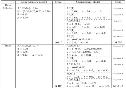
US price inflation can be determined using the GDP index. The dataset used here is available from the Bureau of Economic Analysis, based on quarterly GDP indexes, denoted Pt, from the first quarter of 1947 to the third quarter of 2006 (227 data points). Price inflation is calcu-lated asπt = 400 ln(Pt/Pt−1) (thus n = 226). A plot of the inflation is given below in Fig-ure 2a. Studies of the persistence of this data have been conducted to determine the level of dependence within the series. A high amount of persistence, indicating long memory, was found in [26]. However [19] found a structural break, which when accounted for showed the series to have low persistence, indicating the presence of changepoints with short memory segments. Ap-plying our classification approach to this series will give an additional indication as to which model is statistically more appropriate.
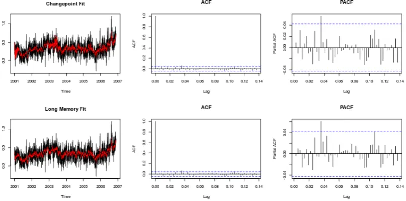
The parameters of the fitted changepoint and long memory models are given in Table 3. Diagnostic autocorrelation and partial autocor-relation function plots are given in Figure 3. The level shifts are given in respect to their
po-sition in the series, but correspond to 1951 Q3, 1962 Q4, 1965 Q2, 1984 Q2. The classifier re-turns a changepoint classification for this series.
4.2 Stock Cross Correlations
Stock Cross Correlation data has been obtained from the supplementary material of [3]. The data consists of Open to Close stock returns for 6 companies from January 1st2001 to 30thJuly 2008 (n= 2156). The data is first transformed using a Fisher Transformation, then correlations are calculated between each stock. Here analy-sis will look at the correlation between Ameri-can Express and Home Depot.
stationarity from [23] (no rejections) and also the fractal R package [4] which implements the Priestley-Subba Rao (PSR) test [27] (time varying p-value 0.061). This coupled with auto-correlation and partial autoauto-correlation function plots given in Figure 4 means we conclude that the segment is stationary. Here the estimated changepoints at times 715, 841, 847 and 896 correspond 15/12/2002, 20/04/2003, 26/04/2003 and 14/06/2003. The distance scores given by the classifier indicate a strong preference for long memory over changepoints. This result stands against that found in [2] which indicated a pref-erence for a model with similarly 4 changepoints. The difference is likely due to the fact that in [2] the changepoint model does not contain any short memory dependence and we have shown here that if that short memory structure is cor-rectly taken into account within the sub-series then the series shows greater evidence of long memory properties.
5 Conclusion
The wavelet classification process presented within this paper provides the user a distinct choice over a number of proposed models, and when explicitly applied to an ambiguity such as long memory or a changepoint as in Section 3, it provides an additional piece of information to aid decision making. The accuracy of the clas-sifier over a number of simulated models has been presented within Section 3 and applied to data from the Financial and Economic fields in Section 4.
The Evolutionary Wavelet Spectrum pro-vides a representation of non-stationarity which is lacking in the commonly used (averaged over time) spectrum. This gives an advantage when drawing comparisons between non-stationary and stationary series, since the wavelet spec-trum may appear substantially different. Quan-tifying this visual difference allows for a direct comparison between the series and each pro-posed model.
The variance-corrected squared distance met-ric used in the proposed classifier has been demonstrated to be quite accurate under the ambiguity of long memory and changepoint mod-els. It is particularly effective at identifying changepoint models correctly, as the results in Table 1 demonstrate. It was noted that there is relatively lower variation between the simu-lations generated for the changepoint than the long memory model, which reduces the distance
metric significantly even though it is variance corrected.
As mentioned in Section 1 there are many series that can be found in fields such as Eco-nomics and Finance which show evidence of the ambiguity investigated here. This classification is not intended to propose a final model for these series, but instead give additional infor-mation, treated perhaps as a diagnostic. This could be to begin investigation of a series, or to confirm a previously found model fit. As this is not a formal test, the lack of assumptions allows for more flexibility in how the classifica-tion can be used. This work however is not re-stricted only to the ambiguity mentioned here, further work could extend it to determine be-tween other features, such as local trends and seasonal behaviour or combining the behaviour of both models i.e., a long memory model with a changepoint.
An aspect not covered in this paper is the precise form of ARMA and long memory mod-els in the LSW paradigm, i.e. how the model co-efficients relate to theWj,k’s. This is an interest-ing area for future research which would cement the LSW model as an encompassing model but is beyond the scope of this paper.
An R package (LSWclassify) is available from the authors that implements the method from the paper.
Acknowledgements The authors would like to ac-knowledge the helpful comments of an Associate Ed-itor, 2 reviewers and Dr. Matthew Nunes. This re-search was conducted whilst Ben Norwood was a graduate student funded by the Economic and Social Research Council in collaboration with the Office for National Statistics.
References
1. Beran, J., J., B.R., Ocker, D.: On unified model selection for stationary and nonstationary short and long-memory autoregressive processes. Biometrika85(4), 921–934 (1998)
2. Bertram, P., Kruse, R., Sibbertsen, P.: Frac-tional integration versus level shifts: the case of realized asset correlations. Statistical Papers
54(4), 977–991 (2013)
3. Chiriac, R., Voev, V.: Modelling and forecasting multivariate realized volatility. Journal of Ap-plied Econometrics26(6), 922–947 (2011) 4. Constantine, W., Percival, D.: fractal: Fractal
Time Series Modeling and Analysis (2016). R package version 2.0-1
5. Daubechies, I.: Ten lectures on wavelets, vol. 61. SIAM (1992)
6. Diebold, F.X., Inoue, A.: Long memory and regime switching. Journal of Econometrics
(a) Time series of US Price Inflation. (b) Time series of the Cross Correlations of American Express and Home Depot.
Fig. 2: Real Data Examples
Long Memory Model Score Changepoint Model Score
Data Inflation
Stock
ARFIMA(4,0,0)
φ= (0.30,0.20,0.20,−0.16)
d= 0.31
µ= 3.29
ARFIMA(1,0,1)
φ= 0.30
θ= 0.58
d= 0.47, µ= 0.35
40147
12128
AR(1)
φ= 0.68, τ= 18, µ= 0 AR(1)
φ= 0.63, τ= 63, µ= 1.70 ARMA(2,1)
φ= (−0.43,−0.33)
θ= 0.47, τ = 73, µ= 1.69 AR(1)
φ= 0.82, τ= 149, µ= 5.43 AR(3)
φ= (0.60,0.19,0.18)
τ= 226, µ= 0 ARMA(4,4)
φ= (−0.05,−0.002,0.07,0.94)
θ= (0.17,0.14,0.04,−0.83)
τ= 715, µ= 0.31 AR(1)
φ= 0.29, τ= 841, µ= 0.42 ARMA(2,1)
φ= (0.09,0.09)
θ=−0.58, τ= 847, µ= 0.30 MA(1)
θ=−0.72, τ= 896, µ= 0.50 ARMA(3,1)
φ= (1.12,−0.06,−0.07)
θ=−0.90, τ= 2156, µ= 0.35
Segment 1
Segment 2
Segment3
Segment 4
Segment 5
38750
Segment 1
Segment 2
Segemnt 3
Segment 4
Segment 5
5348047
Table 3: Model fits and scores for US Inflation (Inflation) and Stock Cross-Correlations (Stock). Bold scores are the minimum. Each segment ending atτ is separated by a dotted line.
7. Fryzlewicz, P., Nason, G.P.: Haar-fisz estimation of evolutionary wavelet spectra. JRSSB68(4), 611–634 (2006)
8. Fryzlewicz, P., Ombao, H.: Consistent classifica-tion of nonstaclassifica-tionary time series using stochastic wavelet representations. Journal of the Amer-ican Statistical Association 104(485), 299–312 (2009)
9. Grabocka, J., Nanopoulos, A., Schmidt-Thieme, L.: Invariant time-series classification. In: P.A. Flach, T. De Bie, N. Cristianini (eds.) Ma-chine Learning and Knowledge Discovery in Databases,Lecture Notes in Computer Science, vol. 7524, pp. 725–740. Springer Berlin Heidel-berg (2012)
10. Granger, C.W., Ding, Z.: Varieties of long mem-ory models. Journal of Econometrics 73(1), 61 – 77 (1996)
11. Granger, C.W., Hyung, N.: Occasional struc-tural breaks and long memory with an
applica-tion to the s&p 500 absolute stock returns. Jour-nal of Empirical Finance11(3), 399–421 (2004) 12. Haeran Cho, P.F.: Multiscale and multilevel technique for consistent segmentation of nonsta-tionary time series. Statistica Sinica22(1), 207– 229 (2012)
13. Hyndman, R.J., Khandakar, Y.: Automatic time series forecasting: the forecast package for R. Journal of Statistical Software 26(3), 1–22 (2008)
14. Janacek, G., Bagnall, A., Powell, M.: A likeli-hood ratio distance measure for the similarity between the fourier transform of time series. In: T. Ho, D. Cheung, H. Liu (eds.) Advances in Knowledge Discovery and Data Mining,Lecture Notes in Computer Science, vol. 3518, pp. 737– 743. Springer Berlin Heidelberg (2005)
[image:9.595.93.503.204.490.2]Economic Dynamics and Control24(3), 361–387 (2000)
16. Killick, R., Eckley, I.A., Jonathan, P.: A wavelet-based approach for detecting changes in second order structure within nonstationary time series. Electron. J. Statist.7, 1167–1183 (2013) 17. Killick, R., Fearnhead, P., Eckley, I.A.: Optimal
detection of changepoints with a linear computa-tional cost. J. Am. Stat. Assoc.107(500), 1590– 1598 (2012)
18. Krzemieniewska, K., Eckley, I., Fearnhead, P.: Classification of non-stationary time series. Stat
3(1), 144–157 (2014)
19. Levin, A.T., Piger, J.M.: Is inflation persistence intrinsic in industrial economies? Working Paper Series 0334, European Central Bank (2004)
20. Michie, D., Spiegelhalter, D.J., Taylor, C.C., Campbell, J.: Machine Learning, Neural and Statistical Classification. Ellis Horwood, Upper Saddle River, NJ, USA (1994)
21. Molz, F.J., Liu, H.H., Szulga, J.: Fractional brownian motion and fractional gaussian noise in subsurface hydrology: A review, presentation of fundamental properties, and extensions. Water Resources Research33(10), 2273–2286 (1997)
22. Nason, G.: Wavelet methods in statistics with R. Springer Science & Business Media (2010)
23. Nason, G.: A test for second-order stationarity and approximate confidence intervals for local-ized autocovariances for locally stationary time series. Journal of the Royal Statistical Society: Series B (Statistical Methodology) 75(5), 879– 904 (2013)
24. Nason, G.: locits: Tests of stationarity and local-ized autocovariance (2016). R package version 1.7.1
25. Nason, G.: wavethresh: Wavelets Statistics and Transforms (2016). R package version 4.6.8 26. Pivetta, F., Reis, R.: The persistence of
infla-tion in the united states. Journal of Economic dynamics and control31(4), 1326–1358 (2007)
27. Priestley, M.B., Rao, T.S.: A test for non-stationarity of time-series. Journal of the Royal Statistical Society. Series B 31(1), 140– 149 (1969)
28. Starica, C., Granger, C.: Nonstationarities in stock returns. The Review of Economics and Statistics87(3), 503–522 (2005)
29. Veenstra, J.Q.: Persistence and anti-persistence: Theory and software. Ph.D. thesis, Western Uni-versity (2012)
30. Yau, C.Y., Davis, R.A.: Likelihood inference for discriminating between long-memory and change-point models. Journal of Time Series Analysis33(4), 649–664 (2012)
A Proof of Theorem 1
Proof We replicate the steps of the proof within the Appendix of [8] up until (A.6), where following this step the short memory condition is used. To briefly
summarise previous steps,
P(D1−D2>0) =P(X−t >0)≤E( ˜X2)/t2,
(by Chebyshev’s Inequality)
E( ˜X2) =:I+II,
I≤CJ0J∗ −J0
X
j=−1 −J∗
X
i=−1
2i+jE
b2i,j ,
E
b2
i,j =: 2A+ 2B.
Definitions for these components can be found in the original proof. Component A is where we alter the proof.
RecallIk,N(i) is the wavelet periodogram at a fixed
scalei, at positionkwith total lengthN, withd(k,Ni)
the wavelet coefficient corresponding to it through
the relationship Ik,N(i) = d(k,Ni) 2. We continue the
proof from (A.6) using the ARFIMA assumption in-stead. Following from above (A.6):
A=E
(N
X
k=1 n
Ik,N(i) −EIk,N(i) ocj,k
)2
≤22j N
X
k,k0=1
cov
Ik,N(i) , Ik(i0),N
= 22j N
X
k,k0=1
2cov2d(i)
k,N, d
(i)
k0,N
(by Isserli’s Theorem) (4)
[15] gives bounds for the covariance of wavelet coefficients;
covd(k,Nm), d(n,Nj) = C1|α|2d−1−2M+R2M+1
α= 2m−jk−n, m≥j
|R2M+1| ≤C2|α|2d−2−2M,
whereM ≥1 is the number of vanishing moments in the wavelet used. Using|α|=|2i−ik−k0|=|k−k0| ≥ 1 and substituting into Equation (4):
A= 22j+1 N
X
k,k0=1
(C3|α|2d−1−2M+R2M+1)2
= 22j+1 N
X
k,k0=1
|C3|α|2d−1−2M+R2M+1|2
≤22j+1
N
X
k,k0=1
(
C3|α|2d−1−2M
+|R2M+1|)2
≤22j+1 N
X
k,k0=1
(C4|α|2d−1−2M
As|α|2d−2−2M ≤ |α|2d−1−2M we have:
A≤22j+1
N
X
k,k0=1
C6|k−k0|2d−1−2M2
= 22j+1 N
X
k,k0=1
C7
1
|k−k0|−2(2d−1−2M)
= 22j+1 N−1
X
s=1
(N−s)C7 1
s−2(2d−1−2M)
= 22j+1C7 "
N
N−1 X
s=1
1
s−2(2d−1−2M)
−
N−1 X
s=1 1
s−4(d−M)+1 #
Given that|d|<0.5 andM ≥1 then 4<−2(2d−1−
2M) =δ1and 3<−4(d−M) + 1 =δ2. We can then replace the sums using the definition of Generalised Harmonic Numbers and their convergence:
Hn,m= n
X
k=1 1
km
Hn,m=O(1) asn→ ∞ (m >1)
Thus
A≤22j+1C7(N HN−1,δ1−HN−1,δ2) = 2 2j+1C
7HN,
whereHN = N HN−1,δ1−HN−1,δ2. Returning to consider (A.4) from [8], we find a bound for compo-nentI, whereJ0, J∗= log2N and∆=
1 (2 log2a−1)
:
I= C8J0J∗ −J0 X
j=−1 −J∗
X
i=−1 2i+j
22j+1C7(N HN−1,δ1
−HN−1,δ2) +N 1+∆2j
= C8log22N −J0
X
j=−1 2j
22j+1C7HN
+N1+∆2j
1−2J∗
= C8log22N
−J0
X
j=−1
C723j+1 1−2J∗HN
+ −J0 X
j=−1
23j 1−2J∗N1+∆
= C9log22N 1−2 −J∗
HN
−J0 X
j=−1 23j+1
+ C8log22N 1−2
−J∗N1+∆
−J0 X
j=−1 23j
= C9log22N 1−2 −J∗H
N 2 7 1−2
−3J0
+ C8log22N 1−2
−J∗N1+∆1 7 1−2
−3J0
= log22N 1−N−1
1−N−3
C10HN+ C11N1+∆
= log2
2N 1−N
−3−N−1+N−4
C10HN+ C11N1+∆
≤C12log22N HN+N1+∆
Following this, using results in [8] the probability of misclassification is:
P(X > t) =O log22N
N−1+N∆−1
Fig. 3: Inflation diagnostics. (Top) Left: Original data with fitted changepoint model; Middle: Auto-correlation Function of changepoint model Residuals; Right: Partial autoAuto-correlations of changepoint model residuals. (Bottom) Left: Original data with fitted long memory model; Middle: Autocorre-lation Function of long memory model Residuals; Right: Partial autocorreAutocorre-lations of long memory model residuals.
[image:12.595.95.504.360.563.2]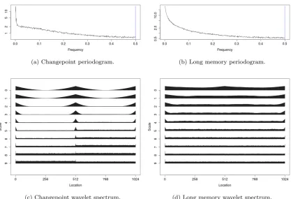
![Table 1: Changepoint observations results with Likelihood Ratio comparison [30].](https://thumb-us.123doks.com/thumbv2/123dok_us/9342403.436263/7.595.125.470.172.396/table-changepoint-observations-results-likelihood-ratio-comparison.webp)