The dynamics of thermostatically controlled loads for power system frequency control

(1)

warwick.ac.uk/lib-publications

A Thesis Submitted for the Degree of PhD at the University of Warwick

Permanent WRAP URL:

http://wrap.warwick.ac.uk/103934

Copyright and reuse:

This thesis is made available online and is protected by original copyright.

Please scroll down to view the document itself.

Please refer to the repository record for this item for information to help you to cite it.

Our policy information is available from the repository home page.

(2)

The dynamics of thermostatically controlled loads

for power system frequency control

by

Ellen Elizabeth Webborn

Thesis

Submitted to the University of Warwick

for the degree of

Doctor of Philosophy in

Mathematics and Complexity Science

Centre for Complexity Science

(3)

List of Tables

2.1 Comparison of centralised and decentralised TCL control strategies . 25

2.2 Benefits and challenges of using TCLs for frequency response . . . . 33

3.1 Parameter values . . . 42

3.2 The number of states and switching events for different numbers of synchronised groups of TCLs . . . 96

4.1 Parameter values for plots in Figures 4.1, 4.2 and 4.3 . . . 105

4.2 Illustrative historic response holding data . . . 112

4.3 Parameter heterogeneity literature survey . . . 137

4.4 Mean and standard deviation for each parameter and diversity factor 139 4.5 Expected parameter range for different percentages of the population for the five diversity factors. . . 140

(7)

List of Figures

1.1 Fuel input for electricity generation in the UK 1920-2016. . . 2

1.2 Solar installation estimates in the UK . . . 3

2.1 Electricity grid transition illustration . . . 9

2.2 Installed generation capacity projections . . . 15

2.3 Frequency-sensitive set points illustration . . . 20

2.4 Different outcomes for a frequency-sensitive refrigerator system . . . 24

2.5 Linearly frequency-dependent temperature set points . . . 27

2.6 Frequency-time control characteristics . . . 29

2.7 Total load demand due to price-based control of PEV loads . . . 32

3.1 Illustration of the Kuramoto model . . . 35

3.2 Visualisingθ . . . 44

3.3 Eigenvalues of the uniformly distributed TCL equilibrium . . . 49

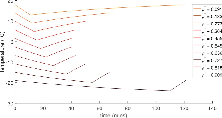
3.4 Fully-synchronised temperature cycling. . . 50

3.5 One cycle of the single group solution . . . 54

3.6 Effect ofβcPc on cycle durations . . . 55

3.7 Phase difference and temperature cycling for synchronising groups, σ= 0.3 . . . 62

3.8 Phase difference and temperature cycling for synchronising groups, σ= 0.7 . . . 63

3.9 Phase difference and temperature cycling for non-synchronising groups, σ= 0.3 . . . 64

3.10 Phase difference and temperature cycling for non-synchronising groups, σ= 0.7 . . . 65

3.11 Phase difference bifurcation diagram for two groups of TCLs . . . . 66

3.12 Four system states and switch events for two groups . . . 67

3.13 All possible events for two groups of TCLs . . . 68

(8)

3.15 Solution for the next group (of 2) to switch in cases 3 and 4 . . . 74

3.16 Initial condition regions for switching event progressions of two groups 78 3.17 Tracking initial temperature pair (3,5) from event A over time for differentρ∗,σ= 0.48 . . . 80

3.18 Tracking initial temperature pairs (3,5) and (10,2) from event E over time . . . 81

3.19 Tracking initial temperature pairs (0,-5) (from I) and (2,7) (from J) over time . . . 82

3.20 Tracking initial temperature pair (3,5) from event A over time for differentρ∗,σ= 0.2 . . . 83

3.21 Two-group linearisation diagram . . . 85

3.22 Solutions for λ(Eq (3.112)) . . . 89

3.23 Bifurcation diagram for the stability of the single group solution to splitting in two . . . 95

3.24 The three types of cycling behaviour of two groups relative to one another . . . 96

3.25 Simplex Coordinates . . . 98

3.26 Long-term behaviour of three groups whenρ∗= 0.3355. . . 99

4.1 Initial fridge distributions in phase . . . 106

4.2 Final fridge distributions after 10 days inθ-space . . . 107

4.3 Electricity grid frequency over 10 days . . . 108

4.4 Simulation methodology . . . 110

4.5 Interpreting historic response data . . . 112

4.6 Cumulative response savings over time for homogeneous populations 119 4.7 Final cumulative response savings for differentPc . . . 121

4.8 Maximum cumulative response savings for differentPc . . . 122

4.9 Time of maximum cumulative response savings for differentPc . . . 123

4.10 Creating a histogram for simulation results . . . 124

4.11 Percentage in each bin for different total fridge load . . . 126

4.12 Temperature spread during simulations for different total fridge load 127 4.13 Final cumulative response savings for different Pc . . . 129

4.14 Maximum cumulative response savings for different Pc . . . 130

4.15 Time of maximum cumulative response savings for different β . . . . 131

(9)

4.17 Percentage in each bin for β = 3.6,4.8,6.0 . . . 133

4.18 Temperature spread during simulations for different total fridge load 134 4.19 Final cumulative response savings for different diversity factors . . . 142

4.20 Maximum cumulative response savings for different diversity factors 143 4.21 Time of maximum cumulative response savings for different diversity factors . . . 144

4.22 Percentage in each bin for diversity factors 0, and 0.25 . . . 145

4.23 Percentage in each bin for diversity factors 0.5, 0.75 and 1 . . . 146

4.24 Final cumulative response savings for different diversity factors . . . 148

4.25 Maximum cumulative response savings withPc= 700MW for differ-ent diversity factors . . . 149

4.26 Time of maximum cumulative response savings for different diversity factors . . . 150

4.27 Percentage in each bin for diversity factors 0 and 0.25 withPc= 700MW151 4.28 Percentage in each bin for diversity factors 0.5, 0.75 and 1 . . . 152

4.29 Final and maximum cumulative response savings for all diversity factors154 4.30 Time of maximum cumulative response savings for all diversity factors155 4.31 Cumulative response savings over time for a heterogeneous population159 B1 Simulation switch time approximation method . . . 167

C1 Summary of stored kinetic energy data . . . 169

C2 Summary of demand data . . . 170

C3 Summary of historic frequency data . . . 172

C4 Summary of high response holdings . . . 173

(10)

Acknowledgments

This thesis would not have been possible without the guidance, support and

inspi-ration of my supervisors, Robert MacKay and Mike Waterson. You have taught me

a great deal and pushed me to become a better mathematician and researcher. I am

very proud of what we have achieved and I’m extremely grateful for your supervision

over the last 5 years. I’d like to thank Lisa Flatley, for all of your encouragement

and assistance with my research, particularly in the early days when I was searching

for research direction. I’m also grateful to the IMAGES research group for support

and stimulating discussions.

To all the people whom I had the pleasure of working with at National Grid, thank

you for helping me to take the leap into the world of engineering, and for teaching

me about the energy industry. I’m particularly grateful to Vandad Hamidi for

supporting me from the start and championing my career at the company. To Matt

Roberts, Roy Cheung and Will Ramsay for your great work with the Frequency

Engine and continued support, which made a huge difference to my simulations,

thank you very much. To Ben Marshall for your generosity of spirit and expertise,

Beth Warnock for your continued encouragement and publication support, and to

everyone in the System Performance team, many thanks.

I have had the privilege of being part of a doctoral training centre full of interesting,

friendly and supportive people. I’d like to thank the many staff and students with

whom I discussed my work and who helped to challenged my thinking. I’ve had great

office mates over the years, Pantelis, Sergio, Chris, Fede, Bernd, Joe, Iliana, Sami,

(11)

chats. Additional thanks go to the Smoothie Club for brightening my Thursdays

with intriguing concoctions, long may it continue.

Although there are too many people to mention by name, and many things I’ll

remember, I’ll take this opportunity to thank a few people who stand out at this

point in time. Thank you Joe for your wit, genuine compliments, and occasional

tough love. Iliana your cakes are amazing and I’ve been touched by your generosity

of baking spirit. Thank you Ayman for your help with Inkscape, and to you and

Michael for letting me use your computer when I was in need of computing power.

Tom and Davide, thank you for being inspirational researchers and friends. Mike,

you always livened up lunchtime discussions with your weird and wonderful debates.

Roger, thank you for your help with simulations and tikz, and for being a wonderful

dance partner. Dancing has been a real source of joy and stress relief, and I’m also

grateful to Josh, Kevin and Nick for being amazing and making me a better dancer

during my time in Complexity. My housemates have always been there for me in

times of celebration and sadness alike. Jamie, Georgia, my Irish boys Barry, Andy

and Conley, also Sophie and Craig, Cyril, Te-Anne and Steph, it’s been a pleasure.

Thank you Dario, for standing by me through thick and thin, always there with

hearty food for late night chats and musical times. Thank you Rachel, who was

there with me when it all began and returned in time to cheer me over the PhD

finish line with tea and friendship.

Finally, I am infinitely grateful to my family, without whom I would not be the

(12)

Declarations

This Thesis is submitted to the University of Warwick in support of my application

for the degree of Doctor of Philosophy. I have read and understood the rules on

cheating, plagiarism and appropriate referencing as outlined in my handbook and I

declare that the work contained in this assignment is my own. No substantial part

of the work submitted here has also been submitted by me in other assessments for

this or previous degree courses, and I acknowledge that if this has been done an

appropriate reduction in the mark I might otherwise have received will be made.

Work contributing to this thesis has appeared in the peer-reviewed publication:

Ellen Webborn & Robert S. MacKay. A stability analysis of

(13)

Abstract

Major changes are under way in our power grids. Until very recently, a few hun-dred, very large, dependable fossil-fuelled power stations were supplying power to consumers whose only role was to use energy whenever they wanted. Today we have wind farms, solar farms, solar panels on millions of roofs, smart metering. Electric vehicles are on the rise and storage technologies are developing rapidly. Achieving a low-carbon, affordable, and secure electricity system, the so-called ‘en-ergy trilemma,’ presents many challenges and opportunities. As en‘en-ergy becomes more dependent on volatile resources such as the wind and sun, flexibility will be-come increasingly important for maintaining system security at palatable costs. One new source of flexibility could come from domestic appliances. Thermostatically-controlled loads (TCLs), such as fridges, freezers, air-conditioners and hot-water tanks are effectively energy stores that can be adapted to meet the needs of the grid with negligible impact on consumers. By allowing their operating set points to vary (a little) according to the electricity frequency, they could provide a valuable re-source to the grid. However, a thorough understanding of their potential to exhibit synchronisation will be needed to understand and mitigate against the potential risks of a decentralised response provider.

(14)

Abbreviations

AC alternating current DC direct current

DSR demand-side response FES Future Energy Scenarios FLC fuzzy logic controller GB Great Britain

GW gigawatt = 109 _{(one billion) watts of electrical power} iff if and only if

kW kilowatt = 1000 watts of electrical power LHS left-hand side

MVA megavolt-ampere = 106 (one million) volt-amperes of apparent power MW megawatt = 106 (one million) watts of electrical power

Ofgem Office of Gas and Electricity Markets PEV plug-in electric vehicle

PHS pumped hydroelectric storage RHS right-hand side

RoCoF rate of change of frequency SO System Operator

(15)

Notation

Symbol Description Units Appears

• denotes on or off depending on the context

- (3.28)

c inverse nominal angular momen-tum

Hz (MWs)−1 (3.12)

c_off f˙ when single group is switched off

Hz s−1 (3.42)

con −f˙when single group is switched

on

Hz s−1 (3.42)

D(t) total measured demand MW (4.1) Demresp f(t), t automatic demand response MW (4.3) Demω0(t) demand at nominal frequency MW (4.2)

Ek(t) total stored kinetic energy MVAs (4.4)

f(t) grid frequency minus nominal frequency

Hz (3.4a)

f− minimum frequency in single

group periodic solution

Hz (3.55a)

f+ maximum frequency in single

group periodic solution

Hz (3.55b)

foff

n grid frequency at timetoffn Hz (3.41a)

fon

n grid frequency at timetonn Hz (3.41a)

GA,GB group A, group B - (3.80) Imbtot(t) total imbalance MW (4.5) Imbunder(t) underlying imbalance MW (4.5)

k dimensionless constant - (3.34)

k0 normalisation constant s−1 (3.23)

l_off off cycle duration of single group periodic solution

(16)

l_on on cycle duration of single group periodic solution

s (3.55a)

L single group periodic solution cy-cle duration

s Figure3.21

N number of synchronised groups - Table3.2

Pc maximum TCL population power consumption

MW (3.12)

S_A, S_B on/off state of group A, group B - Figure3.12

t time s (3.3)

toff

n time of nth switch off of single group

s (3.41a)

ton

n time of nth switch on of single group

s (3.41a)

T(t) temperature ◦C (3.3)

T−0 nominal lower temperature set

point

◦_C ₍_3.4a₎

T− f(t) lower temperature set point ◦C (3.4a)

T₊0 nominal upper temperature set point

◦_C ₍_3.4b₎

T+ f(t)

upper temperature set point ◦C (3.4b)

T_off asymptotic heating temperature (room temperature)

◦_C ₍_3.3₎

T_on asymptotic cooling temperature ◦C (3.3)

TΓ(t) temperature of the single group

periodic solution

◦_C _Figure_3.21

u(θ, t)dθ fraction of TCLs between θ and

θ+ dθ

- (3.18)

v(θ, t) velocity of TCL in θ-space s−1 (3.19)

w(θ, t) perturbation function s−1 (3.29)

woff histogram bin width for switched

off TCLs

- (4.10)

w_on histogram bin width for switched on TCLs

- (4.10)

X∈ {A, ..., L} switch event - Figure3.12

XY switch event progression X then

Y

- (3.89)

(17)

Z0 Z with parameters from

Ta-ble3.1

Hz s−1 (3.40)

α Heating/cooling coefficient s−1 (3.3)

β set point sensitivity to frequency (whenβ− =β+)

◦_{C Hz}−1 ₍_3.60₎

β− lower temperature set point

sen-sitivity to frequency

◦_{C Hz}−1 ₍_3.4a₎

β+ upper temperature set point

sen-sitivity to frequency

◦_{C Hz}−1 ₍_3.4b₎

γ damping factor divided by angu-lar momentum

s−1 (3.12)

δt generator response time lag s (4.7)

∆t time step size s (4.7)

∆P surplus power generation for the TCLs

MW (3.12)

∆t,∆0_t switch on time differences be-tween groups A and B

◦_C _Figure_3.21

∆T,∆0T temperature difference between groups A and B at group B switch on events

◦_C _Figure_3.21

∆u normalised wave peak amplitude - Table4.1

1, ..., 5 time differences in single group

linearisation

s Figure3.21

η(θ, t) perturbation function s−1 (3.27)

θ(t) measure of TCL phase - (3.17)

θn nth normalised phase difference of two groups

- (3.81b)

λ eigenvalue - (3.34)

λ1 eigenvalue - (3.112)

λ2 eigenvalue - (3.134)

µ combination of parameters (Hz s)−1 ₍_3.33c₎

ν0 combination of parameters Hz−1 (3.33a)

ν1 combination of parameters Hz−1 (3.33b)

ξ combination of parameters ◦C s−1 ₍_3.103₎

ξ1 combination of parameters ◦C s−1 (3.114)

(18)

ρ(t) proportion of TCLs switched on - (3.12)

ρ0 expected proportion of frequency

insensitive TCLs switched on

- (3.8)

σ proportion in group A in two group model

- (3.80)

τ_on0 nominal on cycle duration s (3.7a)

τ_on(f) frequency-dependent on cycle duration

s (3.6a)

τ_off0 nominal off cycle duration s (3.7b)

τ_off(f) frequency-dependent off cycle duration

s (3.6b)

φoff(t) combination of parameters Hz−1 (3.21b)

(19)

“I’m absolutely not anti-renewables. I love renewables. But I’m also pro-arithmetic.”

David MacKay,TEDxWarwick, 2012

1

Introduction

Britain, like many countries around the world, is in midst of what could be called an ‘energy revolution’ [1]. In the past year alone there have been headlines such as “GB energy supply enjoys coal-free day for ‘first time since the industrial revolution’ ” [2], “This summer was greenest ever for energy, says National Grid” [3], “Britain opens first subsidy-free solar power farm” [4], and “Jaguar Land Rover to build electric and hybrid new vehicles only from 2020” [5], to name but a few. The public is becoming increasingly aware of, and increasingly involved with, the major changes sweeping the electricity industry.

(20)

[image:20.595.135.516.319.628.2]

electricity generation in the UK between 1920-2016 based on government electricity statistics [6]. Over the last hundred years electricity demand has risen dramatically, and has only recently declined somewhat since its peak in 2005. We can see the rise and fall of coal and oil as our primary electricity sources. Nuclear and natural gas are the largest sources of fuel for electricity today, and other fuels such as wind and solar have been steadily rising since 1990. Figure1.2shows the rapid expansion of solar photovoltaics (PV) over the last eight years to almost 13GW (gigawatt) in October 2017. Wind power has seen similar trends, with current estimates for in-stalled onshore and offshore capacity at 11.0GW and 5.3GW respectively1 [7]. Such widespread changes offer the chance for a future less dependent on fossil fuels [8], but bring with them many challenges to the secure and affordable operation of the electricity grid that are yet to be fully addressed [1,9].

Figure 1.1: Fuel input for electricity generation in millions of tonnes of oil equivalent in the UK between 1920-2016 based on the data in [6].

Our increasing dependence on volatile and less predictable resources such as the

(21)

[image:21.595.136.517.108.383.2]

Figure 1.2: Estimated solar photovoltaics deployment, from [10].

(22)

operation, regulatory frameworks and the design of electricity markets” [11].

The focus of our work is on a particular type of flexible demand. Thermostatically-controlled loads (TCLs) such as fridges, freezers, air conditioners and hot water tanks can effectively be used as energy stores on the grid. They spend periods of time switched on, and periods of time switched off in order to keep food, rooms or water near the right temperature. The precise time when they switch on or off is of no concern to the user, and so their power consumption can be delayed or advanced on the order of several minutes if needed, with no detriment to their operation. To delay consumption is similar to an energy store supplying power to the grid which will be replaced a little later, and to advance consumption is similar to filling/charging a store. By allowing the TCL operating set points to vary a small amount according to the needs of the electricity grid, a population of TCLs can act as a flexible demand resource, similar to energy storage. The rate of change of the grid frequency (RoCoF), detectable anywhere on the network, is an approximate measure of the imbalance between supply and demand. Therefore it would only require a small addition to an appliance to detect the frequency and compute the temperature set points accordingly in order for it to become a flexible resource.

There are a number of challenges with regard to making frequency-sensitive TCLs a reality on the GB grid. For example, there would need to be financial or legal incentives for companies to install the appropriate controllers in existing or new TCLs. Would individual consumers be paid for participating in such a scheme, or would it become a standard component of all new fridge-freezers, for example? If the System Operator were to pay TCLs for providing a balancing service, it would need to know how the population would respond to frequency deviations and be confident that the service could be relied upon. Who would pay if the service did not meet expectations? Beyond the economic and policy considerations, of most interest to us is the control mechanism within each TCL. Many options have been proposed in the literature, but no choice has yet emerged as the optimal solution.

(23)

on and off at the same time. Understanding the propensity of TCL populations to synchronise will be key for avoiding such problems.

The first half of this thesis describes a new continuum model for a population of frequency-sensitive TCLs and presents analyses of the dynamics of a continuum of TCLs, and also of one and two synchronised groups. We consider a simple, decentralised, deterministic control scheme for a homogeneous population of TCLs. Eigenvalue analysis of our model shows that the nominal frequency equilibrium is stable, at least to small perturbations. We also solve for the periodic solution of a fully synchronised group of TCLs. This leads us to study the behaviour of two synchronised groups, which is much more complicated due to the potential for the order of switching (on or off) to change. We analyse the stability of two groups very close to the single group solution, and find the region in parameter space in which the groups will synchronise, and the region in which the groups will separate and remain distinct. This allows us to hypothesize about the long-term behaviour ofN

groups of identical TCLs.

The second half of our work offers a number of simulations which expand on the mathematics and provide new insights into how TCLs would perform on the real GB system under our decentralised, deterministic control scheme. We are able to simulate a large population of TCLs acting on the GB grid using real system data from National Grid from 2015-2016. The data includes system demand, stored kinetic energy, frequency, and frequency response from other providers. To the best of our knowledge, this is the first time TCLs have been simulated with this amount of system data for such long time periods (ten days). In particular, an algorithm from National Grid has allowed us to determine how the other response providers on the system would have acted had the TCLs been frequency-sensitive, and to calculate the resulting reduction (or increase) in response that they were required to provide. We test our theory that with sufficient parameter diversity, a heterogeneous population will avoid the synchronisation issues that befall homo-geneous populations. We discover that even a very small amount of diversity will eradicate these problems. Since diversity exists in any real system, we conclude that the minimal levels required fall within what could be reasonably expected in a population, and so our control scheme is a viable option to implement in a TCL population. Thus potentially unpopular controls with stochasticity can be avoided, as well as infrastructure-intensive centralised control schemes that pose potential security risks.

(24)

de-velopment of a new continuum model describing a population of frequency-sensitive TCLs on the electricity grid. 2) Stability analysis of the nominal frequency equilib-rium in the model. 3) Stability analysis of a fully synchronised group of TCLs to splitting in two and a hypothesis regarding the dynamics ofN groups. 4) Demon-stration that very small amounts of diversity can prevent synchronisation issues in a heterogeneous population, and estimates for the GB system of the potential reduction in frequency response from other providers.

(25)

“Chirping crickets, croaking frogs, flashing fireflies, gaps in the asteroid belt, gener-ators in the power grid-[Norbert] Wiener spotted sync in all of them.”

Steven Strogatz,Sync: the emerging

science of spontaneous order [12]

2

Background

2.1 The Electricity Grid

The first electric power system began operating in 1882 supplying power (for light-ing) to 59 customers in New York City [13]. Today power grids span entire conti-nents, making electric power available to approximately 4.8 billion people [14] and transforming almost all aspects of the way we live. In this thesis, the work is ap-plicable to AC power grids in any country, however we focus predominantly on the electricity grid and current energy policy in Great Britain (GB). We use the terms

electricity grid,power grid,grid and power system interchangeably.

2.1.1 Structure

(26)

load. In addition to generation and load there may also be various types of electricity storage on the network, although in all major power grids (at present), the capacity is relatively small compared to generation capacity. As of 2014 the global installed power generation capacity was approximately 6180GW [15], whereas the installed capacity of pumped hydroelectric storage (PHS), which accounts for over 99% of energy storage capacity, was approximately 127GW [16], a ratio of around 50:1. In Great Britain we have several PHS plants that typically consume electricity at night (to store energy) when demand is low and supply power to the grid during peak times of day. Other key components of an AC power system include power transformers, capacitors, transmission circuits, and control and switching systems1. This description would have been valid 50 years ago and is still relevant today. However, the arrival of renewable power generation, electric vehicles, smart meters and other recent innovations are dramatically altering the way power is generated and consumed. Diagram2.1shows a simplified representation of the electricity grid (a), and the new technologies that we are starting to see connecting to the grid (b).

Today, power is still generated predominantly by synchronous machines that con-vert energy sources such as fossil and nuclear fuels into mechanical energy, driving rotating turbines which in turn produce electrical energy. Alternating current is produced with a frequency equal to the angular frequency of the motor divided by 2π. In order for the grid to operate effectively, all of the generators need to be synchronised, i.e. they all need to be rotating at the same frequency (known as the(electricity grid/system) frequency) so that the phase of the current is the same at all points in the network2. For the purpose of our work we assume that the frequency is the same in all locations. When the power being drawn from the grid is greater than the power being supplied, the generators lose energy and slow down, and this reduces grid frequency. Vice versa, when demand is less than supply, the generators start to speed up and grid frequency increases. In Europe the ideal grid frequency is 50Hz, called thenominal frequency3. The components of any grid are designed to operate within a narrow range around the nominal frequency. They are vulnerable to major faults with severe repercussions for the whole system if the grid frequency deviates outside of this range (approximately 50±0.5Hz).

It is the one of the roles of the System Operator (SO) to ensure that the grid frequency remains within a narrow range of the nominal frequency. Of course,

1

For a detailed description of these components see, for example, [17].

2_{In reality the frequency typically varies a little between different locations, although larger}

differences are sometimes caused by ‘inter-area oscillations’.

(27)

(a) Traditional Electricity Grid

[image:27.595.126.521.109.635.2]

(b) ‘Smart’ Electricity Grid

(28)

the stable and secure operation of the electricity grid involves far more than just maintaining the frequency at its nominal value, for example, careful observance of voltage limits. Many excellent texts can be found explaining in great detail the structure and requirements of the electricity grid, such as Kundur et al. [13] and Eremia and Shahidehpour [18]. In this introduction we focus on the aspects of the electricity grid and system stability most relevant to our work.

2.1.2 Operation

Electricity Markets

Like any commodity, electricity is traded on markets. Domestic electricity con-sumers pay a pre-arranged tariff to companies called suppliers, who procure the electricity from a range of markets. Procurement time-scales range from several years down to one hour in advance of consumption. Unlike other commodities, elec-tricity has very strict constraints on its physical flow from where it is generated to where it is consumed. In order for the electricity grid to operate, the amount of electricity being consumed (bought) must closely match the amount being gener-ated (sold) at all times. This can be difficult to ensure, because predicting national demand ahead of time is imperfect, and generators occasionally disconnect from the system due to faults. Add in the volatility and unpredictability of renewable resources such as wind power and we have a market where few agents know pre-cisely how much power they have to sell, and no suppliers know exactly how much to procure for their consumers. This results in small imbalances between supply and demand, causing the aforementioned physical network challenges. Electricity trading arrangements are therefore designed to incentivise accurate forecasting and to settle inaccurate payments. In this section we introduce the basics of electricity markets and the role of the System Operator (SO) in keeping the grid balanced and secure.

(29)

electricity originated from when it reaches a consumer. What is important is that the total power bought minus sold and the total power consumed minus produced, ultimately balance overall (accounting for transmission losses). The physical bal-ancing of the system is done by the SO which in GB is National Grid, a private company regulated by the Office of Gas and Electricity Markets (Ofgem). National Grid’s role as the SO is to ensure that the system operates safely and securely at all times in the most cost-effective way for consumers. This means redressing any power imbalances and preventing grid instabilities through ‘imbalance settlements’ and ‘balancing services’. Imbalance settlements involve acceptingoffersfrom agents to increase their generation/reduce demand, for a price, and/or acceptingbidsfrom agents to pay the SO to reduce generation/increase consumption4 so that the pre-dicted demand matches the amount procured in the markets [19]. Alongside market balancing, the SO also ensures the physical balancing of the system by maintaining system stability, through the use of balancing services, as we explain below.

Power System Stability

Power system stability is defined by the IEEE/CIGRE Joint Task Force on Stability Terms and Definitions as “the ability of an electric power system, for a given initial operating condition, to regain a state of operating equilibrium after being subjected to a physical disturbance, with most system variables bounded so that practically the entire system remains intact” [20]. Analysis and consideration of this ability is simplified by considering the three classifications of power system stability sep-arately: rotor angle stability, voltage stability and frequency stability. Rotor angle stability refers to “the ability of synchronous machines in a power system to remain in synchronism after being subjected to a perturbation” [20]. Voltage stability in-volves maintaining safe and steady voltage levels throughout the system through reactive power balancing5. As introduced in Section2.1.1, frequency stability is the ability of the system to maintain the grid frequency within a small range of nominal frequency, through supply and demand balancing actions. Frequency stability is the focus of our attention for the majority of this thesis. For more information on the other types of power system stability see, for example, [13] or [20].

A vital part of power system stability (and the analysis thereof) is the concept of

4_{The exception is (currently) renewable suppliers receiving subsidies to generate power, that}

must be paid to reduce generation to cover the loss of earnings from feed-in tariffs.

5

Reactive power is the “energy loaned periodically to the reactive elements in the load”[21] with

frequency twice the grid frequency. For further reading on reactive power, see, for example, [13,21,

(30)

power system inertia. The inertia of a synchronous machine or spinning load is its resistance to changes in its speed of rotation. Inertial/rotational energy is stored in the rotating components of the power system and this inertia must be overcome in order to speed up or slow down the rotation. The heavier the rotating components in a generator or motor (and the greater their distance from the axis of rotation), the greater the inertia [23]. The total system inertia in a power grid equals the sum of the inertia from all synchronised components. A power system with high inertia, such as one with many synchronous generators like coal, gas and nuclear will naturally have greater frequency stability, since changes to the supply-demand balance take longer to affect the system due to the high inertia. When system inertia is low, for example in a system with many asynchronous components such as solar panels, wind turbines and DC interconnectors6, the system is more sensitive to frequency changes, and therefore stability is lower. The anticipated reduction in system inertia over the next few decades [9] is part of the motivation behind our research into how domestic appliances can play a role in supporting system stability. Very closely-related to system inertia is the stored kinetic energy in the system. System inertia is a more commonly discussed concept in the literature, but the data we will use in Chapter 4 includes the stored kinetic energy of the system, rather than system inertia. They are related by the equationEk = 1₂Iω2, where I is total inertia andω is angular velocity.

Balancing Services

Balancing services are a range of options available to the SO to mitigate against unexpected changes in supply or demand and potential faults on the transmission or distribution system. Typically the procurement of balancing services involves paying a generator or consumer to be prepared to act if a fault occurs on the system, or to act continuously to keep the system prepared for such an event. In this section we describe the current set of balancing services in Great Britain [25].

The SO is required to maintain system frequency withinstatutory limits(50±0.5Hz) and, in the absence of incidents such as generator outages or power line faults, within

operational limits (50±0.2Hz). This is achieved by employing different types of

frequency response7. The most common types of frequency response service

6_An_{interconnector}_{is an electricity link between power grids in different countries. For example}

in GB there are currently four interconnectors, to France (2GW), to the Netherlands (1GW), to

Northern Ireland (0.5GW) and to the Republic of Ireland (0.5GW) [24].

7

(31)

available to the GB System Operator, National Grid, are

• Mandatory Frequency Response: most generators are required to provide this

service in order to connect to the grid. There are three types:

– Primary Response: increase power output/decrease demand within 10 seconds of a frequency incident,8 sustained for a further 20 seconds if required

– Secondary Response: increase power output/decrease demand within 30 seconds of an event and sustained for 30 minutes as required

– High Response: reduce power/increase demand within 10 seconds of an event and sustain indefinitely (as required)

• Firm Frequency Response: procured via a tendering process, a provider must supply at least 10MW of energy as either:

– Dynamic Response: continuously varying output in response to frequency deviations away from 50Hz

– Static Response: delivery of a pre-determined increase/decrease in power output when the frequency hits a set level (step-function response)

• Frequency Control by Demand Management (FCDM): industrial/commercial consumers are paid for the interruption of their power supply for thirty min-utes, typically thermal appliances such as supermarket fridge-freezers or hotel air conditioning systems

• Enhanced Frequency Response (EFR): a new service that requires a full re-sponse within one second of an event. The first tendering exercise was held in July 2016, when 200MW of EFR was procured from various energy storage providers.

Based on the current power system conditions such as system inertia, time of day, and the largest power generator/interconnector power supply to the system that could be lost due to a fault, National Grid procure a combination of these services from months to hours ahead of real time.

On longer time-scales (minutes to several hours)reserveservices are used to support the system. Reserve services have a longer start-up time than frequency response

8_{A frequency incident/event is a sudden change in the power balance, such as when a line or}

(32)

services, and in some cases are initiated manually. There are three main types of reserve:

• Fast Reserve: response within 2 minutes of an event, increasing power/decreasing demand by a minimum of 25MW/minute and providing at least 50MW of power

– Required to be highly reliable and paid to be constantly ready for an event

– Typically used to take over from frequency response providers and to support ‘TV pick-ups’ (demand spiking due to television scheduling)

• Short-Term Operating Reserve (STOR): provision of at least 3MW of gener-ation or demand reduction within 4 hours of instruction and sustained for at least 2 hours

• BM Start-Up: Balancing Mechanism Units (BMUs) which were not scheduled to run can be procured to be made available to National Grid for reserve.

Additional types of service includereactive support, current and developing de-mand side response services and constraint management services. More in-formation can be found on all of the above balancing services on the National Grid website [25].

2.2 Renewable Energy

Faced with the threat of climate change, many nations have been setting targets to reduce carbon emissions. For example, the UK government has committed to reduc-ing emissions by at least 80% of 1990 levels by 2050 [26]. To reduce our dependency on fossil fuels, we have seen a huge surge in the development of renewable energy and so-called ‘smart’ technologies, such as smart metering in homes, electric vehicles, and various forms of energy storage. As technologies become more cost-effective, ei-ther through technological advances, mass-production or government subsidies, they are becoming increasingly prevalent on the GB power grid. Such changes naturally bring a mixture of challenges and opportunities for system operability, which must be carefully navigated. Anticipating changes to demand and generation and the potential issues requiring mitigation is part of the role of the SO.

(33)

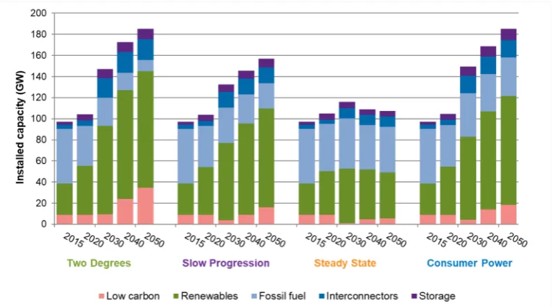
projec-tions for the changes to energy supply and demand in the coming decades, based on input from stakeholders from all areas of the energy industry. The 2017 scenarios (projections to 2050) are

• Two Degrees (TD) - high economic growth and investment in green

technolo-gies and strong government policy to drive change, the only scenario in which the UK meets its carbon targets

• Consumer Power (CP) - high economic growth, lower focus on green

govern-ment policies, market-led investgovern-ments in smaller generation with shorter-term financial returns

• Slow Progression (SP) - low economic growth competes with desire to meet carbon targets, cost-effective long-term environmental policies

• Steady State (SS) - low economic growth, business as usual, security of supply

at low cost, little investment in long-term solutions, the ‘least-green’ scenario.

Figure2.2shows the projections for the installed capacity of each class of generation for each of the four scenarios. We see a moderate-to-large increase in the installed capacity of renewables in all four scenarios. The role of interconnectors and storage also increase, as the amount of installed fossil-fuel generators reduces.

Figure 2.2: Installed generation capacity projections by type, for each energy sce-nario in the 2017 FES [27].

[image:33.595.123.519.429.649.2]

(34)

an electricity grid that arise from increased use of renewable energy, in particular wind power and solar PV, such as [1,9,28–31]. The key operational challenges for a grid with a high penetration of renewables (or distributed renewables) are reduced inertia, greater RoCoF (Rate of Change of Frequency), fewer generators capable of providing frequency response, voltage fluctuation and harmonic distortion, power quality issues, and the supply volatility and unpredictability caused by the nature of the weather. The challenges most relevant to our work are the first three, which directly impact the electricity grid frequency and/or the need for greater frequency response.

As discussed above, the higher the system inertia, the slower the system will be to grid frequency fluctuations. To provide inertia to the system, a component must be synchronously connected (rather than connected with a power electronic converter). To provide a significant amount of inertia, the component needs to have large rota-tional inertia, such as a heavy motor or a turbine in a power plant. Solar panels have no moving parts and therefore contribute no inertia to the system. Wind turbines and interconnectors are connected via power electronic converters, and so at present they are unable to supply system inertia. With lower inertia the frequency changes more rapidly. When the RoCoF is high, the load-shedding controller will decouple its component(s) from the system to protect them. Certain renewable technologies such as solar PV are particularly sensitive to high RoCoF and in the event of a fre-quency incident may remove themselves very quickly from the system, exacerbating the frequency issues.

Traditionally energy was generated by a relatively small number of very large power plants, such as coal, oil and gas. In recent years energy generation has become far more distributed, meaning that we now have a large number of very small generators on the distribution network with a large spatial distribution. These generators are often invisible and beyond the control of the SO9. They can also dramatically alter the way power flows in the distribution network, since bi-directional flows become possible. In recent years decentralised generation has grown to comprise over a quarter of installed capacity in GB. National Grid’s Future Energy Scenarios [32] anticipates that this percentage will increase to 34-40% by 2025 and to 34-50% by 2050. According to their analysis, to achieve the UK carbon targets would require the highest percentage in each of these ranges.

The analysis presented in National Grid’s System Operability Framework 2015 [9]

9

(35)

predicts a number of challenges for frequency control going forward. System inertia is expected to reduce over the next 20 years in all four future energy scenarios during periods of low demand and/or high renewable power generation. Primary frequency response requirements are expected to increase by 30-40% by 2020, and new response providers will be needed to meet these requirements.

2.3 Smart Grids and Demand Response

Alongside the recent advances in renewable technologies is the development of the ‘smart grid’ concept. According to EPRI, “The term ‘Smart Grid’ refers to a mod-ernization of the electricity delivery system so it monitors, protects and automati-cally optimises the operation of its interconnected elements – from the central and distributed generator through the high-voltage transmission network and the dis-tribution system, to industrial users and building automation systems, to energy storage installations and to end-use consumers and their thermostats, electric ve-hicles, appliances and other household devices” [33]. To some, the term ‘smart grid’ is something of a clich´e, over-hyped and over-applied. However, it is useful to distinguish between the centrally-controlled, generator - network - consumer power flow model of the 20th century, and the vision for future electricity systems with greater complexity and control schemes. This is not to say that current (or past) power grids lacked intelligence. Indeed, complex software and automated routines are essential parts of what is an incredibly complex system, that in many cases, spans thousands of miles and/or millions of homes. Rather, by integrating new electrical and communications infrastructures that allow greater participation and support from distributed resources, such as domestic batteries or electric vehicles, the grid will become smarter. In the words of Borlaseet al. “A truly modern smart grid would include sustainable concepts that leverage proven, cleaner, cost-effective technologies available today or under development” [14].

A key part of any smart grid is demand-side response (DSR)10. DSR refers to a change in a consumer’s (or an appliance’s) normal electricity demand at a certain time, in response to an incentive or control from a supplier or SO. Dehghanpour and Afsharnia [34] classify five types of demand response services:

• Energy efficiency servicesimplement energy saving technologies to reduce

de-10

(36)

mand through efficiency savings

• Price response programs incentivise consumers or automatic controllers to

schedule or interrupt demand (typically appliances such as washing machines or dishwashers) to consume power at cheaper times of day, where price may depend on prices paid by suppliers or needs of the electricity grid

• Peak shaving programs spread out the total load at peak times to reduce the maximum energy requirements of the system each day

• Regulation responseemploys centralised control to assist with power balancing

on a highly frequent basis

• Frequency response (spinning reserve) schemes employ centralised or decen-tralised (through local measurements) control to provide demand response in real time, on very fast time-scales.

Each type of response may have an important role to play in the future of the smart grid, as flexibility becomes more important to the system. In this thesis we concern ourselves with the final type of DSR; the potential to use demand-side appliances for the provision of dynamic frequency control.

2.4 Frequency-Sensitive

Thermostatically-Controlled Loads

2.4.1 Introduction

A thermostatically-controlled load (TCL) is an appliance/device whose operation is controlled by a thermostat. Examples include fridges, freezers, air conditioners, hot water tanks, heat pumps and swimming pool pumps11. They operate to maintain a status quo, such as keeping food, water or a building at a roughly constant tem-perature. Unlike other appliances such as kettles, televisions and electric lighting, users pay little or no attention to whether their TCLs are switched on or off, and have no preference, so long as the proper temperature cycling continues to maintain the room temperature, food freshness or hot water availability. This means that the exact time at which a TCL switches on or off in its cycle is relatively flexible, and it is this flexibility that renders them potential providers of DSR.

11_{Although not strictly operated by a thermostat, swimming pool pumps operate in the same}

(37)

Although controlling a large population of small appliances brings new challenges such as control schemes and service/remuneration designs, in addition to being a potential resource that already exists, there are also benefits from using an aggre-gated resource compared to a single large DSR provider. For example, very fast, continuous responses are possible in ways that are not always possible with a single machine. Spatially distributed TCLs have the potential to redress local fluctuations before they create problems at the system level [35]. It can also be argued [36] that availability and reliability is improved when splitting a service between a multitude of providers, compared to a single unit which will become completely unavailable in the event of a fault or scheduled repair. It is estimated in [37] that around 40% of total demand in Europe comes from household appliances, of which fridges and freezers make up 15%, electric storage water heaters 9%, and air conditioners around 1%12. Therefore, although individually TCLs consume very tiny amounts of electric-ity (relative to say, the power generated by a gas power plant), as a large population, they have the potential to make a meaningful contribution to demand-side (and of interest to us, frequency) response.

As explained above, the electricity grid frequency is primarily affected by, and is therefore a measure of, the difference between total supply and demand on the system. Ensuring the frequency remains as close as possible to 50Hz (the nominal frequency) requires keeping supply and demand closely matched at all times. TCLs operate between two temperature set points, switching on when one is reached, and remaining on until the temperature hits the other set point. Normally these set points are fixed, unless a user interferes with operation, which is relatively rare. Figure 2.3(a) shows an example temperature trace of a cooling device such as a fridge. In this hypothetical case the fridge spends 20 minutes switched on until it reaches its lower set point when it switches off for 40 minutes.

Electricity grid frequency can be sensed anywhere in the network, and a TCL with a frequency sensor has the capability to provide sub-second response to a fluctua-tion [38]. We can make a TCL frequency-sensitive by allowing the set points to vary according to some function of the grid frequency. Continuing the example above, we would want the fridge to consume less power when the frequency is less than 50Hz and more power when the frequency is higher than 50Hz. Consuming less power means increasing the set points so that the fridge stays off for longer or switches off sooner in its cycle. Consuming more power requires the opposite. Figure2.3(b)

12

(38)

gives an illustrative example of frequency-sensitive operation of a fridge. Exactly how the temperature set points depend on the frequency is an important part of any control design.

(a) Normal TCL operation (b) Frequency-sensitive TCL operation

Figure 2.3: Illustration of how TCLs normally operate (a) and how frequency-sensitive temperature set points could increase/decrease the power consumption of a population by advancing/delaying switching of individuals.

(39)

reduced reliability in procuring services from thousands of very small demand-side resources, which is undoubtedly an obstacle to be overcome. Effects on consumers and their appliances will be of concern to potential participants. Finally, it will be crucial for the success of any scheme to adequately address the requirements for minimum participation numbers and to develop the right business models that ensure fair rewards and effective incentives.

Research into the possibility of using TCLs for grid balancing services began in the 1980s with key papers such as [48–52]. The changing energy landscape of the 21st century has brought a new focus to the use of TCLs for electricity grid support and a wealth of literature on the topic [34,35,41,45–47,53–78]. Work has varied in nature from mathematical frameworks to numerical simulations and real-world trials. Most of the theory can be applied to any type of TCL, and simulations have touched on many types of TCL technology. A variety of control schemes have been proposed, from centralised, direct-load control to completely distributed, autonomous load control. An important obstacle to the introduction of TCLs for frequency response, in particular, is the propensity for TCL temperature cycling to become synchro-nised. This can be triggered by frequency deviations that become reinforced and cause system instabilities. In the remainder of this section we introduce synchro-nisation phenomena in a general setting, summarise TCL synchrosynchro-nisation evidence and discussions in the literature, and describe the different types of control schemes that have been proposed.

2.4.2 Synchronisation

(40)

explain. One such class of emergent phenomena is synchronisation.

Synchronisation Phenomena

Firefly colonies stretching miles in SouthEast Asia have been observed to flash in unison to awe-inspiring effect. Audiences in eastern-European theatres applaud and the applause becomes a beat of clapping in unison. Walkers on the Millennium Bridge in London were initially found to cause major oscillations on the bridge as their footsteps started falling in rhythm. Simple oscillators with no centralised control spontaneously synchronise their cycles to great effect [12]. In some cases the phenomenon is beautiful, mystifying to the casual observer, impressive to behold. In other cases the effects can be devastating.

Power grid stability relies on generator motors rotating in synchrony in order to prevent inter-area oscillations and large frequency perturbations [80, 81]. Mod-elling power grids as collections of coupled oscillators has gained recent attention in physics [82–87]. These references describe a simplified power system using the Kuramoto framework and assess the stability of the system. For example, [83] considers the impact of decentralising power on system stability and finds that self-synchronisation is still possible and that decentralised grids are “more robust to topological failures”. The authors in [86] establish a synchronisation condition for a general class of coupled oscillator models and in particular apply their results to power networks. In contrast to the work that follows on synchronisation with a population of TCLs, power grids depend on synchronisation in order to operate se-curely. For a population of generators, synchronisation is highlydesirable, and work such as the aforementioned references attempt to improve how quickly and robustly a network can synchronise. As explained below, the synchronisation of TCL cycles is exactly what needs to beavoided.

Synchronisation in TCL Populations

(41)

appliances, we may start to see spikes and troughs in the load as TCL population switching behaviour starts to cluster temporally. This would have a destabilising effect on the system, and lead to an overall detrimental impact on system stability. The simulations in [69] do not find evidence of synchronisation, however, we be-lieve that this is largely due to the heterogeneity in the simulated TCL population. The population was divided into 1000 groups to be modelled separately, and each group “was randomised by altering every parameter to within ±20%”. An impor-tant contribution of this thesis is to explore the effects of heterogeneity on TCL synchronisation.

A number of simulations in the literature indicate TCL synchronisation following a frequency disturbance, for example [53, 60, 61,65,69–71]. Of particular signifi-cance is the 2012 publication by Angeli and Kountouriotis; A Stochastic Approach to “Dynamic-Demand” Refrigerator Control [53]. Building on the work of Short et al.[69], the authors highlight the possibility for synchronisation and the resulting system instabilities through simulations. In one case the authors simulate the effects on a homogeneous fridge population of a 1.32GW power loss lasting 15 minutes be-fore a 10 minute ramped power recovery. It should be noted that while a 1.32GW loss is possible on the GB grid, fast reserve services would begin to make up for some of the loss after around 2 minutes, rather than the 10 minutes assumed. Under the proposed control scheme in [69], the resulting deviations in system frequency and re-frigerator power consumption indicate “overall unstable behaviour” and undesirable effects for the fridges and the system. The authors also offer theoretical arguments for the long-term tendency of the system towards TCL synchronisation. It is rea-soned that any “small periodic ripples in power system frequency will gradually entrain oscillations of refrigerators that have similar frequencies of oscillation, thus reinforcing the frequency ripple and eventually leading to an even larger number of entrained refrigerators”.

As the title suggests,Emergent synchronisation properties of a refrigerator demand side management system by Kremers et al. [61] and their subsequent book chap-ter [60] explore this topic in some detail. The authors use an agent-based model of frequency-sensitive refrigerators with greater detail than in the aforementioned research. For example, stochastic door opening and the impact of fridge contents on temperature are considered. They find three possible types of outcome with the same parameters due to the stochastic nature of their model, as shown in Figure2.4.

(42)

Figure 2.4: Taken from [61]: “Examples of different regimes of the refrigerator system. On top, the total load curve of the refrigerators and below the corresponding grid frequency. The simulations were performed with the same parameters. Due to the non-deterministic nature of the model and for the given parameterisation, each of the three regimes can appear”.

after having switched off to support a large frequency deviation. Although synchro-nisation is observed in the heterogeneous population (unlike in [69] where it is only hypothesized), the control scheme used in [60,61] is significantly different. Rather than allow the temperature set points to vary continuously in time with the grid fre-quency, the refrigerators are switched off at a specific frequency point, and switched back on following a significant frequency drop at another. The benefits of the first control scheme are that the appliances best-positioned in their cycle respond fastest to the needs of the grid13. In the event of a frequency incident (a sudden significant drop in frequency caused by, say, an unexpected loss of a large generator), all ap-pliances switch off at exactly the same time, and will reconnect at exactly the same time. We believe that this is a significant contributor to synchronisation observed in the simulations, and accordingly choose our analysis of frequency-sensitive temper-ature set points as the means to implement demand-side response. Some of the key aims of our research are to determine whether a homogeneous population of TCLs will always be at risk of synchronisation, and to what extent (if any) introducing heterogeneity can mitigate this risk.

13

(43)

2.4.3 Control Strategies

[image:43.595.123.517.278.618.2]

In recent years a number of different types of control strategy for TCLs to provide frequency response have been proposed, many of which are discussed and compared in [34, 46,74]. There are two main classes into which these types of TCL control schemes can be divided: centralised and decentralised control (with a spectrum in between). Their key features and comparative advantages and disadvantages [34] are summarised in Table2.1.

Table 2.1: Comparison of centralised and decentralised TCL control strategies. In-formed by, for example, [34,88].

Centralised Control Decentralised Control

Key Features • TCLs instructed by a cen-tral controller

• Autonomous local control

• 2-way communication in all TCLs

• Control scheme established once, may be updated period-ically

Advantages • Highly controllable • No communications infras-tructure required

• Reasonably predictable • No security risks

• Very fast response possible Disadvantages • Establishing and

maintain-ing a secure communications network are very expensive

• Response is less predictable than with centralised control

• Response time limited by communication speed

• Synchronisation and insta-bility effects possible and not yet fully understood

• Vast amounts of data to manage

• Errors and noise in local frequency measurements more likely

• Data and appliance control security risks

• Negative public perceptions of external control of home appliances

(44)

envi-ronment that was extended to a heterogeneous population through perturbation analysis [50]. A criticism of models such as [49–52] is that their complexity and lack of general closed-form solution renders them unsuitable “to be effectively used by well-understood feedback control design methods” [67]. It is noted [67] that these difficulties appear to be the reason why so many of these models are open-loop control (for example [49–52, 70]). In reality the power system feels the direct impact of TCL response and so closed-loop control models are preferable. When a centralised controller issues instructions to TCLs, these instructions do not have to be influenced by the resulting TCL behaviour, and so typically the control is open loop. Conversely, the decentralised control approaches of interest to us are closed-loop control; the system is affected by the TCL response behaviour which in turn impacts the control scheme in each TCL. Decentralised control strategies are discussed in greater detail below.

An exception to open-loop control is the work by Callaway in [57] which, developing the framework in [50], proposes manipulation of the temperature set points by a broadcast signal from a feedback controller. The approach is applied specifically to air conditioners to support wind smoothing14. Closed-loop dynamics are also cap-tured in the aggregate TCL response models proposed in [68,75] for heterogeneous populations of air conditioners.

It is widely accepted that if millions of TCLs could be used for frequency response they could potentially provide a valuable resource for the system. However, if each device needed constant communication with a central controller, sending data about its temperature and switching history and receiving operation instructions, the eco-nomics and security risks would severely outweigh the benefits of the service. Public perception of the service is also vital for the implementation of any control scheme that involves appliances in people’s homes. For these reasons we choose to focus on decentralised control for our research. A better understanding, however, of the po-tential undesirable side-effects of decentralised control is required before any control strategy could be put in place.

14_{Wind smoothing is the varying of supply or demand to smooth out the natural fluctuations in}

(45)

Deterministic temperature set point control

The simplest form of decentralised TCL control is to change the TCL temperature set points according to some deterministic function of system frequency. The ad-vantages are that simple rules require little processing and the TCLs in the best position to respond to frequency deviations respond first, allowing those that are least ready to wait a little longer before altering their preferred behaviour. In 2007, Short, Infield and Freris publishedStabilization of Grid Frequency Through Dynamic Demand Control [69] which inspired and influenced a significant body of work in this area. The authors simulate the operation of 1320MW of non-identical fridge-freezers responding to large deviations in grid frequency and fluctuations in wind power. They propose a control scheme whereby the TCL temperature set points are linearly dependent on the grid frequency. Figure 2.5 (reproduced from [69]) shows the difference between the normal operation of a fridge and the devised linear frequency-sensitive control scheme proposed. When the frequency is higher than 50Hz the temperature set points decrease, allowing the fridges to switch on sooner or stay on longer, thereby advancing power consumption to meet the generation surplus causing the frequency rise, and vice versa when the frequency drops be-low 50Hz. Shortet al. conclude that the use of many TCLs in this way “has the potential to provide significant added frequency stability to power networks, both at times of sudden increase in demand (or loss of generation) and during times of fluctuating wind power” and “may result in considerable cost savings” [69]. It is perhaps unsurprising, then, that this initial study of TCLs for frequency smoothing led to a surge of interest from the research community.

(46)

The challenges with this type of control are the aforementioned potential synchro-nisation issues, and in our work we attempt to fully explore these issues and look to solve them through the addition of heterogeneity to the TCL population.

Stochastic temperature set point control

In order to prevent synchronisation in a population of TCLs with decentralised control, many papers introduce stochasticity into the control scheme. Typically this takes the form of randomising switch on times following a response action or randomly switching a TCL on or off in addition to the normal control rules. For example, Xuet al.[47] simulate a heterogeneous population of electric heaters in the Nordic power grid using fixed frequency threshold response and the deterministic control proposed in [69], with the addition of stochasticity in two of the control pa-rameters. They uniformly distribute the frequency switch-off thresholdfoffbetween 49.85 and 49.90 Hz and uniformly distribute the time to switch back on following a drop in frequency belowfoff between 4 and 6 minutes.

Molina-Garc´ıa et al.[66] use a distributed frequency-threshold control approach to model a heterogeneous population of different types of TCL. Figure2.6indicates the control approach - frequency deviations ∆f are allowed to exist without response for a short period of time τ. Larger deviations cause response more quickly than small deviations, and depending on the type of TCL different threshold limits can be applied. TCL protection rules prevent devices from remaining switched off for too long or switching off too soon after a TCL switches back on following response. After the minimum recovery time the time of the next switch off is randomised to prevent TCL synchronisation.

In their 2012 paper [53] Angeli and Kountouriotis model domestic fridges as Markov-jump linear systems where the on/off switching is governed by transition probability rates rather than temperature set points. These rates are determined by choosing the desired population average temperature or duty cycle and the temperature prob-ability density is steered towards a desired distribution. The authors show that their algorithm “yields a locally asymptotically stable closed-loop system, regardless of parameter values and control gains” [53]. They also eliminate the ‘payback’ phase (overshoots from fridges recovering lost energy following response actions). How-ever, as noted in [72], in fully eliminating the payback phase the recovery time is longer for each device and rapid response is less feasible. In their 2013 paper Aunedi

(47)

ben-Figure 2.6: Individual load controller ∆f-time characteristic (left), average charac-teristics for different types of TCL used in simulations (right), reproduced from [66].

efits of frequency response under the control scheme proposed in [53] in which the switching probabilities are optimised to prevent overshoots and instabilities. Addi-tional hybrid control schemes are proposed, such as introducing safety temperature thresholds to prevent the fridges from exceeding their preferred temperature range, and making these thresholds frequency-dependent, to increase response speed for large frequency deviations.