Essays in volatility research

(1)

ESSAYS IN VOLATILITY RESEARCH

by

TRISTAN LINKE

MSc in Quantitative Finance, Lancaster University (2011)

THESIS SUBMITTED TO THE DEPARTMENT OF ACCOUNTING AND FINANCE

IN PARTIAL FULFILLMENT OF THE REQUIREMENTS FOR THE DEGREE

OF

DOCTOR OF PHILOSOPHY IN FINANCE

at

THE MANAGEMENT SCHOOL,

LANCASTER UNIVERSITY

2017

c

Tristan Linke, MMXVI.

(2)

Thesis Advisor:

Prof. Ser–huang Poon, Professor of Finance

External Examiner:

Prof. Nick Taylor, Professor of Finance

Internal Examiner:

(3)

(4)

This thesis has been written during my time as a Ph.D. candidate in Finance at Lancaster

University and as a visiting Ph.D. scholar at the Econometrics Department of the

Univer-sity of Amsterdam. This Ph.D. thesis starts with an introduction to finance for a general

audience. Followed by an extensive literature overview, which I have continued to enrich

over the years, of interesting topics in the econometrics–intense field of finance so I felt

the need to incorporate it into my Ph.D.—which is a documentation of my work over the

last years. I then start with a very brief teaser regarding finite sample properties of the

classical skewness estimator and a robust alternative. This paves the way to the first paper

in this thesis on Realized Skewness, Asymmetric Volatility and Risk Management which

is co–authored with my supervisor and was influenced by my time spent in Amsterdam.

The next paper, asymmetric dynamics in index volatility and constituent correlation was

my first work after completing my M.Sc. in Quantitative Finance at Lancaster University

on jump detection methodologies. It largely developed during the first period of my Ph.D.

with the great support of my supervisor and my thesis advisor. These two papers are

linked by an overarching theme: the asymmetric effects of returns on future volatility and

vice versa. The last chapter, co–authored with Cisil Sarisoy, developed more recently and

concentrates on transformations of the covariance matrix, also known as the beta, in a

(5)

PREFACE

Acknowledgements

Of course this thesis would not have existed if it were not for the support from so many

different people over the years. I would here like to take the opportunity to thank in

particular my supervisor Stephen J. Taylor for his invaluable guidance, his advice with

applications, and his insightful contributions to our joint research projects.

Without knowing of my existence, Stephen already guided me through my

undergrad-uate thesis on volatility spreads at the ESB Business School through his book Asset Price

Dynamics, Volatility and Prediction, which ultimately draw me into the newly opened

master degree programme in quantitative finance at Lancaster and I felt like Robert Cole

visiting Ibn Sina in the book the Physician by Noah Gordon when he offered to supervise

me for my M.Sc. and later on for my Ph.D. dissertation. Very special thanks also goes

to my thesis advisor Ser–huang Poon at Manchester Business School who was guiding me

very well and shared lots of interesting research ideas over the course of my studies and

providing me the opportunity to present my work at Manchester, and to my sponsor at

the University of Amsterdam Peter Boswijk, who enabled me to stay for nine months at

the University at Amsterdam and always seemed curious in my research and gave many

insightful comments and suggestions for improvements. I would also like to thank Mark

Shackleton and Ingmar Nolte for guiding me through the literature and commenting on

many research ideas and for their open door policy.

The Department of Accounting and Finance at Lancaster University, the Department of

Econometrics at the University of Amsterdam, and the Department of Finance at

Manch-ester Business School have all been very stimulating and interesting environments to work

in. The great seminar series and brown bag seminars have been very inspiring for my

work. I am also grateful for the financial support throughout my studies provided by the

Department of Accounting and Finance at Lancaster, the scholarship by Lancaster

Uni-versity Management School, scholarshop by the Northwest Doctoral Training Center of the

ESRC and in particular I would like to thank Steve Young or enabling me to teach on the

departmental programmes, and the trust in me in supervising several master dissertations.

No matter where I have been, I have had the privilege to be surrounded by great

Ph.D. colleagues, and I have very much enjoyed their company during this endeavor.

Thank you to my officemates Rui Fan, Xi Fu, Yang Liu, Andrei Lalu and in particular

(6)

Lastly, I wish to thank my friends, my parents and my sister for your patience and

support over the years, and for bearing over with me being slightly absentminded at times.

Declaration

This thesis is submitted to Lancaster University in support of my application for the degree

of Doctor of Philosophy. It has been composed by myself and has not been submitted in

any previous application for any degree. The work presented including data generated and

(7)

Introduction

Introduction to the Financial Economic Setting

IN REAL–LIFE we are exposed to a variety of possibly interrelated risks as is the case

in the domain of finance with the difference being that in the latter case risks may be

directly tradable. If so, one should reasonably expect those risks to be priced, albeit in

sometimes fragmented markets through in–transparent market mechanisms with divers

market participants trading at different time horizons both in terms of execution and

holding period.

In the case of exchange–listed as opposed to over–the–counter traded financial

instru-ments researchers can more easily obtain a set of information from which a priced

com-pound risk premium can be inferred provided the underlying (pricing) model is correct.

Model misspecification plays in fact a very important role but it also raises notoriously

difficult questions to answer, which is why it often remains unaddressed.

Risk premia are then further related to economically interpretable risk factors whose

individual, relative contribution to total risk and, thus the absolute exposure to risk may

well change over time.

The variation in returns calculated from a financial asset price process is non–stationary.

It is stochastic. Although theoreticians may argue that when conditioning on the realized

asset price path the variation might in fact be deterministic and, going further, piecewise

constant. The investor faces exposure to the instantaneous states such as variance, derived

from a relatively short realized asset price path, and to the stochasticity thereof. However,

we can still gain insights when simplifying assumptions are made. Particularly over long

horizons time–varying volatility becomes less important.

Recent financial econometric work has also brought forward evidence that theoretical,

(12)

jumps, which are superimposed upon an otherwise continuous realized asset price path.

Whenever these are non–diversifiable, analogously there should exist a premium based

on the prevailing instantaneous arrival rate, i.e., the probability of occurrence, its size

distribution, and for the stochasticity thereof—in terms of intensity and parameters related

to its size distribution. Currently, there is an ongoing debate regarding the contribution

of discontinuities to the total variation of the price price process, ranging from 20% to

only 1% percent—depending on how inference is conducted, and where these jumps occur

in parameterized models. The equity (price) risk premium can then be understood as the

compendium of exposures to risks.

From a macrofinance perspective, risk premia can be linked to macroeconomic variables

and preference parameters such as risk aversion. Hence establishing a link between the

macroeconomy and asset prices in a joint way. Moreover, there is a strand of literature

trying to link the aversion of the economic agent with the uncertainty attached to asset

prices and hence establishing an intuitive link between the dynamics of asset prices and

uncertainty aversion. Based on this, models of macrofinance should provide insights and/or

generate the dynamics of asset prices.

It is important to remind ourselves that all price models are approximations to the

unknown stochastic process which generates observed prices. Financial econometric

em-piricism and financial economic theory are rarely advanced at the same time, both of which

can progress substantially without relying too much on the other while eventually each

disciplines the other. Measurement is important as it builds the foundation and key

in-puts for theoretical models which are built towards isolating signal in noiseless, controlled

settings.

This thesis focusses in great detail on the measurement part, in particular on the

dynamics and co–dependencies between asset price paths and volatility in univariate,

bi-variate and in simplified multibi-variate settings.

Financial Econometric Rationale for Chapters 1, 2, 3

Chapter 1: Realized Skewness, Asymmetric Volatility, and Volatility Feedback

(13)

gen-erated by the underlying asset price dynamics and their relation to one another through

non–linear transformations. The second moment has received a great deal of attention over

the last decades from the recognition of its time–varying nature to linking innovations in

measures of variation back to realizations in the return residual process with dependent

innovations either occurring concurrently or lagged. It then depends on the sampling

frequency and noise inherent in the data whether the econometrician is able to correctly

identify and moreover correctly specify the underlying economic interdependencies of

func-tions of the return generating process.

Lead lag co–variation terms of functions of returns and spot variation naturally extend to the definition of skewness: It is key to recognize that the asymmetric nature of the link between realizations in the return residual process with innovations in

the variance process and vice versa explain the stylized facts regarding the third moment

and its non–linear transformation such as skewness which we document and explain here

from both a measuring point of view in noisy settings and from a theoretical model based

(parametric) point of view.

Parsimonious univariate measures: Aggregate multivariate constructs, in which stocks are weighted constituents of large index tracking portfolios, are generally more

parsimo-niously modeled and measured in their univariate form due to errors–in–variables issues

when aggregating estimates of large multivariate systems under the alternative. The

uni-variate way in which we propose to measure non–parametrically certain functional forms

of the third moment under very mild assumptions in Chapter 1 is in congruence with that

line of thought, both at the index level and at constituent stock level.

Harvesting the Realized Methodology: We extend the class of estimators belonging to the realized methodology framework from a previous focus on measures of variation to

the aforementioned measures of co–variation between functions of returns and spot

vari-ation which extend to the definition of skewness, here and henceforth denoted realized

skewness estimators. Existing proposed increasingly noise–robust and more efficient

esti-mators, under certain assumptions, are applied, examined and compared in terms of their

results for realized skewness estimates. Note that the conventional measure of skewness is

a subset of the realized skewness estimator suggested here under simple assumptions and

(14)

aggrega-tional properties of the data generating process under certain assumptions. As such the

information set is richer which is again reflected in a smooth evolution of realized skewness

estimates as a function of extending return horizons compared side–by–side to the

conven-tional measure of skewness, which evolves erratic and noisy. The convenconven-tional measure of

skewness suffers from the small sample size, in which the sampling frequency dictates the

measuring frequency as we explain later on, which would result in large standard errors

when the return horizon is long.

Empirical Findings: From an empirical perspective, we examine the contribution of the three components, i.e., the instantaneous skewness, asymmetric volatility, and

volatil-ity feedback, to total realized skewness for various proposed model–free realized skewness

estimators across different sampling frequencies ranging from five to 55 minutes for index

returns and constituent stock returns. We show how at the stock market index level

re-alized skewness builds up over time, becoming more negative, and then slowly decreases

in magnitude towards zero. While for stock market index returns asymmetric volatility

appears to be the main driver of realized skewness across sampling frequencies and

real-ized skewness estimators, which makes it an interesting candidate for the reduced–form

semi–parametric realized skewness estimators, the attribution for constituent stocks looks

different: We classify stocks into distinct realized skewness categories based on

attribu-tion by the three components (stocks with asymmetric volatility, stocks with asymmetric

volatility and volatility feedback effects, stocks with large instantaneous skewness and

stocks whose return multi–horizon return distribution appears to be largely symmetric).

Remarks: While we show in a theoretical way by relying on an extension of a standard commonly applied parametric model how skewness builds up over time in line with

stan-dard assumptions of the data generating process, we do not explicitly derive the stanstan-dard

errors of this class of parametric reduced–form estimators at this stage. However, these can

be derived from stated moment conditions. The application of the proposed reduced–form

parametric estimators becomes interesting when the researcher is willing to superimpose

structure on the data generating process without necessarily being willing to truly belief

in or estimate the most restricted version, i.e., the full parametric model.

Recall that the realized methodology framework relies on within trading day open

(15)

we do not pursue at this stage, the proposed reduced–form estimators can be extended to

include these terms and resulting cross–terms under the assumption that the correlation

structure estimated from intraday data remains intact and applies. Then, overnight terms

and cross–terms are simply scaled by the variances of non–open market period returns.

Chapter 2: Reconciling Asymmetric Dynamics in Index Volatility and Constituent Correlations

Upon the relevance of ARCH–type models: Autoregressive conditional heteroske-dasticity–type models are still very much the workhorse in the domain of finance for

practitioners and academics beyond the narrow focus group of financial econometricians

alike—due to the models tractability, (quasi) maximum likelihood estimates are readily

available, and modeling dynamics in multivariate settings (portfolios) can easily be broken

down into univariate estimation of the volatility series with variance targeting and leaving

much flexibility to impose almost any correlation structure on standardized (or simulated)

residuals.

Realized measures are interesting in the sense of being able to observe an estimate of

variance conditional on the realized asset price path, particularly as realized variance has

been shown to be a credible proxy for the variance of open–to–close returns, i.e., under

empirically realistic conditions, the conditional expectation of quadratic variation is equal

to the conditional variance of returns (Andersen, Bollerslev, Diebold, and Labys, 2003,

Corollary 1), which could be further extended to allow for overnight returns (Hansen and

Lunde, 2006). However, realized variance does not yield an asset price dynamic generator

and it is instead used as a plug in estimate in ARCH–type models or HAR–type reduced

form volatility models, where in the latter case further assumptions need to be made to

produce a financial economic (asset price) scenario generator as in Fan, Taylor, and Sandri

(2017).

Frequency Domain Considerations and Temporal Aggregation: Empirical finan-cial econometric research and findings evolve along with the availability and depth of the

transaction history records. High frequency data for constituent stocks are only available

since approx. two decades from the mid 1990s, with credible high frequency data for only

the most liquid stocks for a much shorter time period. Once the research interest extends

(16)

intraday data.

The benefit of using daily and less coarse data frequencies are that single–period returns

sum up to multi–period returns as there are no gaps in contrast to using intermittent high

frequency data. Note, however, that both applications exercise interesting use cases: While

the former addresses the exposure that an investor faces over the course of consecutive

trading days when closing out her position over night, the latter case is applicable for a

long term investor who stays invested over longer periods of time. ARCH–type models

do not temporally aggregate, meaning that when estimated at one frequency and then

simulated, the properties of multi–period returns do generally not equate to those that

follow from the same model which is estimated at a lower frequency theoretically; refer to

Drost and Werker (1996) for continuous time GARCH diffusions instead.

However, this property serves as a useful control mechanism when inference is

con-ducted at different sampling frequencies; bearing in mind that point estimates of

param-eters come with a standard error which is larger when less data points are used and that

the information set overall is smaller when sparse sampling is applied. Still the properties

of the data generating process which we are interested in here hold for those sampling

fre-quencies at which the models are estimated respectively such as daily and weekly returns.

For properties of multi–horizon returns the analysis in the previous chapter shall lead to

more easily interpretable results as, e.g., the skewness of the density of monthly returns

based on the simulation of estimated ARCH–type models at more granular frequency may

be misspecified.

Asymmetric Volatility & Asymmetric Constituent Correlations Methodology:

We consequently set out in Chapter 2 to explore the inherent dependence structure among

constituent stocks in order to reconcile the large magnitude of asymmetric volatility

re-sponse at the aggregate portfolio (index) level with the less pronounced univariate

asym-metric volatility effects at the individual stock level.

We revert to univariate estimation of model based conditional asymmetric volatility

based on its own univariate residual process. We also tested to include lagged market shock

residuals as explanatory variable(s) in each constituent’s heteroskedasticity process. The

rationale for doing so rests on the observation that (asymmetric) ARCH–type processes

were originally designed to be used at the index level and consecutively applied one to one

(17)

parameters of common stock variance processes is related to negative market residuals

which turns out not to be strongly supported by the data; this part is thus excluded from

the analysis for brevity but available upon request.1

The most common choice for asymmetric ARCH–type models are the EGARCH model

(Nelson, 1991) and the GJR–GARCH model (Glosten, Jagannathan, and Runkle, 1993)

with the main difference being in the news impact curve and the benefit of ensuring

positiv-ity without imposing additional constrains for the exponential garch formulation. While

we test other specifications, we focus on these models which have proven to withstand

the test of time and to save ourselves from (joint) data and model dredging. In order to

ensure ourselves against potentially flat likelihood objective functions and thus numerical

convergence issues, we estimate parameters based off a vast dimensional grid of starting

value and also test parameters estimates from previous rolling windows, which results in

several hundred thousands of estimation sets.

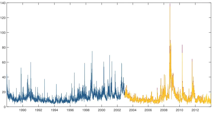
For index and constituent data covering almost one century, we estimate univariate

conditional variance models based on forward rolling ten year windows at daily and weekly

sampling frequency. The window size is chosen in order to balance having a large enough

sample size for these observation driven models while keeping the horizon short enough to

reasonably ensure stationarity

In order to facilitate the analysis of showing how asymmetric constituent correlations

lead to asymmetric volatility effects at the aggregate portfolio level, inference results need

to rely on exactly the same information set of index returns and constituent returns.

We address this issue in several ways by a novel reconstitution methodology: Firstly, as

the Dow Jones Industrial Average is a price weighted index, we create two additional

indices. An equally weighted index rebalanced daily and a market capitalization index

rebalanced daily—both keeping track of stock splits, mergers, name changes, new issuances

etc. Sampling takes place at the daily level which can be aggregated to coarser frequencies

such as weekly. Note that at each rolled forward estimation date we get the Dow Jones

constituents as of that date and create both equally weighted and market capitalization

weighted portfolios of these constituents over the backward looking ten year period.

We then propose one simple estimator of the average threshold exceedance correlation

across all portfolio constituents, where the threshold can be set to zero or specified as a

1_{In continuing research, we have started to extend the framework to allow for asymmetries using the}

(18)

function of standardized constituent residuals. This natural estimator conditions on the

estimated constituent return series volatilities but is otherwise intentionally left

uncon-ditional. The estimator can thus be used as a constraint in constructing portfolios via

constituent selection and weight optimization which minimizes the downside exceedance

correlations in an unconditional way for long term investors that does not active market

timing.

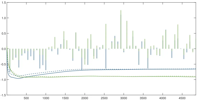
Empirical Findings: Since the asymmetric components in conditional volatility mod-els were first discovered in the 90s, we witnessed a gradual and strong increase in the

asymmetric effect at the index level, which holds for all major US stock market indices,

to the extend that almost all future updating of the one step ahead conditional variance

comes from negative lagged return residuals.

To the best of our knowledge, for the first time we go beyond that time period and

document that there have been equally high asymmetric periods throughout the 1900s

and the magnitude of the effect is time–varying—this is robust against a range of

alterna-tive asymmetric specifications which are available from the author upon request, but not

reported here for brevity except for the GJR and EGARCH specification. We also note

that the effect is more pronounced at the weekly sampling frequency opposed to the daily

sampling frequency which is in line with the results in the previous chapter. The effects are

weaker for individual firms than for aggregate portfolios: Correlations between constituent

returns increase when the market falls, which explains the higher index asymmetry. Thus

the index has more asymmetry than the firms. Asymmetry has increased over the last

three decades both for the index and the mean firm.

Chapter 3: The Role of Noise in the Estimation of Betas

The variance and bias trade-off: In the last Chapter, we consider the relation between classic OLS betas and realized betas: It has been an interest to use highly frequent data

in estimating assets’ sensitivities to systemic risks, β, in order to benefit from statistical precision gains.

(19)

pling frequencies higher than 20 minutes still leading to a significant bias towards zero.

Sheppard (2006) further revisits two models for their ability to explain common empirical

regularities finding that for standard models where prices are contaminated with

stochas-tically independent noise are unable to explain the behavior of realized covariance as the

sampling frequency increases.

However, we show that when the prices are contaminated by i.i.d. microstructure

noise, estimates of the betas are biased and derive a closed–form expression for it. The

estimates are biased towards zero, the magnitude of the bias rises with sampling more

frequently. We conduct a simulation analysis to examine the properties of the estimates

of the betas. We demonstrate that there is a trade-off caused by bias and the variance

and lead to an optimal sampling frequency (in the RMSE sense) among a wide range of

frequencies examined. We conduct a simulation analysis as we were not yet able to derive

the optimal sampling frequency analytically.

Financial Econometric Literature Review

Before we proceed to the three core chapters, we will review relevant financial econometric

building blocks that should help the reader to put the thesis and its contributions into

the relevant context. As the first and second chapter both focus on asymmetric volatility

and skewness we view it as more parsimonious to conduct one large literature review

in the introductory chapter rather than having two largely repetitive literature reviews

in this thesis. We start by reviewing stochastic volatility models which leads us to the

model considered in Chapter 1: While we do not feature discontinuities in an otherwise

smooth model, we favour a discrete exponential multiplicative component volatility model

with can likewise produce very rough paths. As many stochastic volatility models are

driven by the intend to more adequately option price dynamics we also review this strand

of literature incl. non–parametric risk–neutral skewness research from implied volatility

curves. Eventually real–world and risk–neutral dynamics should be theoretically connected

but it is hard to quantify the exact linkages. 2 We then review the measurement theory and applications falling under the realized methodology as it is relevant to understand

the realized skewness estimator we propose in Chapter 1 under the various asset price

dynamic assumptions (jump diffusion setting etc.). We then turn to ARCH–type models

2

(20)

in univariate and review multivariate settings which sets the analysis in Chapter 2 into

the appropriate context. We conclude the literature review with economic explanations

regarding the asymmetric volatility and skewness empirical regularities.

In volatility research we can broadly distinguish three mutually influencing and now

partly overlapping concepts: One, stochastic volatility; two, autoregressive conditional

hetereoskedasticity–type models; three, forward–looking option–implied volatility. More

an underlying theme than a modelling technique influencing all three areas is the

sam-pling frequency which has evolved from daily to intraday data (high frequency up to one

minute), tick data (ultra high frequency below one minute). There is always a trade–off

be-tween non–trivial residuals which may arise due to (complex) microstructure noise at high

frequencies vs. loss of information at low frequencies and inefficiencies due to transaction

costs.

A Brief Note about Time Deformation

Inspired by Houthakker, Mandelbrot (1963) first established the notion of volatility

clus-tering, whose associated non–stationarity property of the return generating process has

also been perceived by Black and Scholes (1972) in empirical tests of their option pricing

formula. Probably also due to the elegance of their derivation and a not well–defined

economic understanding of the variance risk dynamics, the detected apparent anomaly

has not been considered as significant enough to impact pricing and outweigh transaction

costs at that time and was consequently neglected. Almost twenty years later, Mandelbrot

(1982) briefly comments on his seminal 1963 work re–emphasizing how his approach based

on invariance principles decouples prices formation from investor inertia and fits constant

jumps and swings without necessarily having to introduce (time–varying) co–dependence

among the model building blocks, which might have in turn motivated Merton’s (1976)

idiosyncratic jump-diffusion model with constant instantaneous (an average implied)

vari-ance.

The financial economist Clark (1973) introduced the theoretical idea of Bochner’s

(1949) time–deformed Wiener process Wτ, as both a latent and a deterministic func-tion of variables such as trade volume, into finance. Assuming independence in W and

τ, log returns p are a mixture of normal distributions when observed in calendar time,

pt=Wτt → pt|τt∼N(0, τt). Follow up articles include Tauchen and Pitts (1983), who

(21)

the number of active traders, Andersen (1996), who allows for informational asymmetries

and liquidity effects to impact the trade process in response to news, and Ane and Geman

(2000), who advocate the number of trades as a better proxy for market activity in their

jump–diffusion framework. Recently, Andersen, Bondarenko, Kyle, and Obizhaeva (2015)

find that return variation per transaction is log–linearly related to trade size in contrast

to previous studies which are trying to relate volatility to transaction counts or trading

volume.

The trading frequency explained through a time deformation from calendar to asset intrinsic time by the opportunity to execute a trade either independent of volume or as a fixed amount of e.g. shares outstanding/ percentage of free-float should in the long run not

influence the intrinsic value of that share as all business activities take place in calendar

time.

More importantly, the time deformation viaτ is simply a non–negative, non–decreasing, non–autocorrelated process which introduces variation in volatility but cannot distinctly

address empirically observed volatility clustering.

Foundations of Stochastic Volatility

Origins of Stochastic Volatility: The first published research on stochastic volatility with clustering effects induced by autocorrelation can be found in Taylor (1980, 1982) in

which returns are modelled as a non–linear product process of the form

Rt−µX =Vt·Ut,

where volatility shocks Vt are always positive via setting Vt = exp(ht/2) with ht+1 being an AR(1) Gaussian white noise process, i.e.

ht+1 =µ+φ(ht−µ) +ηt.

Ut, a zero mean unit variance process, determines the news impact effect in magnitude and sign. The random variables ηtand Ut are here assumed to be independent. Relaxing this assumption yields a model which can deal with asymmetric effects and produce different

levels of skewness as a function of the horizon. The discussion takes place in discrete time

and motivated by the fact that news are produced at a finite rate. Extensions of the model

are widely used today such as in Huang and Tauchen (2005), Barndorff–Nielsen, Hansen,

(22)

Stochastic Volatility in Continuous Time: The continuous time equivalent to the model above, which also addresses asymmetries and thus skew effects, is the Hull and White

(1987) model, building on Vasicek’s (1977) application of a mean–reverting Ornstein–

Uehlenbeck process in modelling interesting rates. Hull and White write the variance

process in the two forms shown in below, where ω is a scaling factor,

dσ2=α(σ2)dt+ω(σ2)dW,

dlog(σ2) =α(µ−log(σ2))dt+ωdW, α >0.

The Heston (1993) model theoretically overcomes the drawback of obtaining negative

values (as previously encountered in the standard Hull–White variance process above) by

modeling a square–root process. For St the diffusion process andvt the variance process we write the model in real-world dynamics as

dSt=µStdt+

√

vtStdz1,t,

d√vt=−β

√

vtdt+δdz2,t,

where µ is the drift parameter, dz1,t is a standard Wiener process correlated with dz2,t via ρ and scaled by √vt. Itˆo’s lemma applied to second equation above yields the CIR variance process. The risk–neutral stochastic dynamics for the log asset price ln[St] =xt can thus be summarized as

dxt=

h

r−1

2vt

i

dt+√vtdz1,t,

dvt=κ[θ−vt]dt+σV

√

vtdz2,t,

where κ is the mean–reversion parameter, θ the long–run mean of the variance, and σ

the volatility of volatility parameter. When Euler discretization is applied to the variance

process negative values can be obtained. In such cases the variance can either be set to

zero or inverted. Other methods include sampling from the exact transition law of the

process. However, when the discretization step is very small, negative values are hardly

obtained and there are virtually no biases arising.

(23)

markets dominated by long hedgers. Furthermore, the specification equips the

condi-tional return distribution with excess kurtosis and BS IV curves with concavity increasing

w.r.t. |ρ|and σV, and IV curves can both be upward or downward sloping depending on the initial value at V0; see Das and Sundaram (1999) for respective volatility smile and smirk properties; refer to the following subsection: Risk–Neutral Skewness from Implied

Volatility Curves.

Heston–type models still serve today as the workhorse for volatility modelling, see

Gatheral (2005). The application might not yield an adequate description of the asset

price dynamics but obtained estimates are often accurate proxy enough to determine

reasonable option prices due to high bid–ask–spreads and investor’s willingness to pay

for protection. Via Fourier inversion the solution is available in closed form making it

particularly attractive. In practice, the model is often re–calibrated daily to only match

option prices, i.e. minimize option pricing errors, at a target maturity.

The Heston (1993) Fourier inversion of the conditional characteristic function to

cal-culate risk–neutral expectations in closed form encouraged the theoretical development of

new models with rare jumps in prices due to the following shortcoming of the model.

Deutsche Bank (2002) states that in unconstrained parameter estimation Heston–type

models barely match the earlier addressed Feller (1951) constraint and even if matched

in appropriately calibrated market models the distribution of realised variance is highly

peaked near zero with a heavy tail. Market calibration is consequently only achieved by

outweighing the probability of long low volatility periods with very high volatility

proba-bilities Jaeckel (2002). In the various available estimation methods using price and options

data, the correlation coefficent |ρ|is assigned high values (≥0.7) to produce the distinct skewness. In terms of variance risk requirements such a high variance–spot correlation

has not been verified by econometric analysis. Among others, Benzoni (1998) rejects the

specification as skewness and excess kurtosis cannot be simultaneously matched. Another

related issue occurs with the earlier addressed peaks in the distribution of realised variance

at low levels which can be circumvented by increasing the mean–reversion parameter to

in-crease convergence speed towards an assumed ”core stationary distribution” (in a mixture

of distribution setting), see Fouque (2000) for an empirical work. While this approach has

the advantage to allow for temporary variance upsurges it will be even harder to replicate

(24)

Multi–factor Stochastic Volatility Models and Jump Processes The smile of Black–Scholes implied volatilities is consequently indicating the heavy–tailed risk–neutral

distribution. Bates (1996) is probably the first influential study which showed the need to

incorporate a jump component in the price process with regard to FX data; followed by

Scott (1996), Bates (1997), Scott (1997), Chernov and Ghysels (1998), Pan (1998), Bakshi

et al. (1997, 2000), Bakshi and Madan (2000) and many more.

Duffie, Pan, and Singleton (2000) specify a general class of affine jump-diffusion models

which is adaptable to the Qmeasure using their proposed transform theorem. Their

gen-eralized affine stochastic volatility model with state-dependent, correlated jumps (SVSCJ)

for the logarithmic asset price process, Pt=log(St), solves:

dPt=µt,p dt+

p

Vt−dW1,t+JtPdNtP,

dVt=κ(θ−Vt−)dt+σV

p

Vt−

ρdW1,t+

p

(1−ρ2₎_dW

2,t+JtVdNtV,

where for the càdlàg (continué à droite, limité à gauche) specificationVt−= lims↑tVs, the drift parameter µt,p has locally bounded variation and Wt is standard Brownian Motion in R2 for which the scaled diffusion terms in dP and dV are correlated via a constant

instantaneous correlation coefficientρ. Consequently, the instantaneous log price variance process is modelled as a one–factor square–root process plus a (counting) Poisson process

N_tV modelling the occurence of jumps with magnitudes coming from the distributionJ_tV.

N_tP is a Poisson process generating jumps in the asset return process, whose size follows the distributionJ_tP. For a complete definition and characterization of the affine framework we refer to the very technical document, Duffie (2003).

As special case of the affine class proposed by DPS, Barndorff-Nielsen and Shephard

(2001), henceforth BNS, suggest pure non–Gaussian (positive) jump processes of

Ornstein-Uehlenbeck type as the building blocks for volatility models. In the simplest form they

write the following SDE for the variance process

dσ_t2=−λσ_t2dt+dz(λt), λ >0,

wherez is a non–negative process with independent and stationary increments. Volatility can then be modelled as a weighted sum of independent Ornstein–Uehlenbeck processes

with different persistencies. From their equation we can see that the autocorrelation

(25)

This can be regarded as the L´evy response to Comte and Renault (1998)’s long–range

de-pendent stochastic volatility model where the log volatility is constructed via fractional

Brownian Motion. Interesting and stimulating for further research is also Section 6.3 in

BNS, which outlines the idea to directly link tick–by–tick data to their proposed model

dynamics; resorting to the framework by Rydberg and Shephard (2000). For more

exten-sive research into option pricing using the BNS model I refer to Nicolato and Venardos

(2003).

In a series of papers Carr, Geman, Madan, Wu and Yor generalise the time–changed

stochastic process idea proposed by Clark (1973) to a general L´evy process. Starting at

zero, any increasing pure jump process is suitable to model the time–deformed random

clock as time cannot turn negative; I suppose unless we model the instantaneous (log) time

change instead of determining the passage of time directly. Carr, Geman, Madan, and Yor

(2003) state that the clock would be locally deterministic in the absence of jumps. Ruling

out this undesired feature, it can be concluded that jumps in time then trigger jumps in

the asset price process. An equivalent argument requiring a diffusion component in the

price process is not obvious (ibid.).

Early on in their study, Geman, Madan, Yor (2001) remind us that diffusions should

only be applicable in the case where prices adjust continuously to the information flow

resulting in instantaneous equilibria. Discontinuous information flow should thus be

mod-elled by discontinuous stochastic processes exhibiting finite variation unlike Brownian

Mo-tion. Under this new setting jump–diffusion can be interpreted as infinite–activity3 pure jump processes of finite variation where large innovations exhibit a lower (finite) intensity

than their smaller complements. From my point of view the question remains why there

should be infinitely many jumps instead of a finite number per time interval.

The resulting model can be linked to dependently and heterogeneously occurring

eval-uations of a continuous diffusion process in which the random evaluation times can itself

show dependence to the price process. Consequently, when the intensity rate is high

enough continuity can emerge in anactivity–based measure of time which does not need to hold for the price process in calendar time. Interesting is their modelling of the price

process as the difference between two increasing, here gamma, processes, one for price

increases with mean and varianceµ1, ν1 and one for price decreases withµ2, ν2 such that

3_{For a high–activity level the price is non–constant for all time intervals, however the arrival rate for}

(26)

the log price process pt is described as

pt= ν1

µ1

γ

µ2

1

ν1

t

− ν2

µ2

γ

µ2

2

ν2

t

,

where γ is a unit mean and variance gamma process.

Carr, Geman, Madan, Yor (2002), henceforth CGMY, empirically investigate into index

and equity return dynamics and suggest that indices tend to be well described by an

infinite–activity pure jump process with finite variation under both the real–world and

risk–neutral measure as potentially existing idiosyncratic diffusion risk contributions from

individual stocks seem to be diversified away. However, CGMY impose caps at a lower

boundary for very small changes and respectively an upper boundary for large changes in

approximating the finite activity process to minimize the degree of equivalence between

the measure. The cost and the potential impact of doing so onto the measure change

from real–world to risk–neutral remains unclear to me at this stage. Further CGMY put

forward an interesting and intuitive hypothesis that open interest in OTM puts might be

a plausible cause of the negative skewness observed in option–implied distributions (ibid

p.307), which moves the discussion towards equilibrium rather than arbitrage pricing.

In contrast to BNS (2001) who focused on variance modelling exclusively, i.e. the price

process process is still driven by Brownian Motion, the previously addressed studies are

obviously concerned with a joint modelling of the price and variance process as a pure

jump process in terms of a simple homogenous L´evy framework. Consequently, Carr,

Geman, Madan, and Yor (2003) introduce the BNS modelled features such as

asymme-tries and mean–reverting volatilities into their time–changing process which governs the

discontinuous L´evy process—primarily to match option prices across maturities.

Due to the distinctly separate modelling of price and variance processes in stochastic

volatility models and subsequently encountered difficulties in theoretical and econometrical

work even for univariate models, multivariate models are not widely spread in the SV

domain—the exception probably being Fiorentini et al. (2004) which is based on the

discrete–time model by Diebold and Nerlove (1989). It has influenced asset pricing factor

models when volatility clusters.

Risk–Neutral Skewness from Implied Volatility Curves

(27)

match mid quotes of exchange traded options at one maturity on individual stock and

plotted against a simple, non–standardised moneyness measure,4 exhibits a ’smile’, i.e. is almost symmetric, at short horizons and a ’smirk’, i.e. is asymmetric, at longer horizons.5 To overcome truncation, discretisation, extrapolation biases, which arise when

approx-imating the continuum of option prices from sparse discrete data, Jian and Tiang (2005,

2007) recommend to fit cubic splines to mid prices of index option trades and quotes over

a simple but wide moneyness range.

Gatheral and Jacquier (2004, 2005, 2012, 2013) come up with a flexible parametric

specification of the volatility surface which aims at eliminating static and recently also

dynamic arbitrage jointly at multiple maturities in the presence of stochastic volatility

and jumps. Such a formulation enables us to further analyse the dynamics of the implied

volatility surface in terms of their model parameters with regard to dynamics of the

un-derlying security. Bedendo and Hodges (2009) employ discrete and linear Kalman filter

updating of the volatility skew and assess the models capability of producing good density

forecasts. They claim an outperformance of their model compared to the sticky–delta and

vega–gamma alternatives. Zhang and Xiang (2008) employ a second–order polynomial

function to quantify the implied volatility curve and then relate level, slope, and curvature

coefficients to the properties (cumulants) of the implied risk-neutral distribution of asset

returns and show how such links can be used to calibrate and compare different option

pricing models.

The slope of an implied volatility curve or differential slopes of left (out–of–the–money

put) vs. right (out–of–the–money call) ’wing’ of the implied volatility curve set in relation

to at–the–money implied volatility ultimately determine but do not directly equate to

the standardised third moment, i.e. skewness, of the risk–neutral return distribution.

By building on the Bakshi and Madan (2000), Carr and Madan (2001) result on how to

replicate any claim from a continuum of option prices in the cross–section of moneyness

of one asset at one target expiry (T −t), BKM show how to replicate implied moments, moreover, implied skewness and implied kurtosis of the risk–neutral return distribution,

henceforth RNS and RNK, over that forward–looking horizon (T −t).

4_{such as}_K/X_,_log₍_K/X_{) where}_K _{denotes strike price and}_X _{denotes spot or future price} 5

(28)

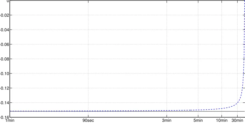
Approximating RNS at Index and Stock Level: Slopes of individual equity op-tions are much less negative than the index (Bakshi, Kapadia, Madan (2003) as equivalent

analysis of options on stock indices such as the S&P500 reveals a strongly pronounced

asymmetry at short horizons which is in turn almost flat at very long horizons under the

same (simple) moneyness measure. It seems to be yet unclear whether these results hold

in the case of standardised moneyness measures such as Black–Scholes–Merton (BSM)

delta.6 E.g. Wu (2012) provides some, although weak empirical evidence for index im-plied volatility curves as a function of BMS delta resembling the shape of a smirk also

at long horizons. Robust inference at long horizons is especially hampered when the

cov-ered standardised moneyness range measured by e.g. BMS delta is shrinking over time

even when the range of covered strike prices remains unchanged, which is the case under

usual market conditions for index and individual stock options. Then, tails of the risk–

neutral density can no longer be spanned by option prices and the density is consequently

truncated, not necessarily symmetrically.

Neumann and Skiadopolous (2012) make repeated use of smooth cubic splines over

a truncated delta grid to obtain constant implied maturity moments for S&P500 index

options. The integrals are evaluated using trapezoidal approximation. The authors further

note that extrapolating in the time dimension creates artificial spikes in implied moments

from which they refrain themselves. However, in absence of a formal sensitivity test thereof,

consequently created large gaps in the time series of constant maturity moments7 can themselves lead to spurious spikes. The CBOE implied volatility and skewness reference

indices VIX and Skew Index are both calculated based on a discrete strike grid with two

consecutive zero bid option prices as cut–off rule for the strike price range and linear inter–

/extrapolation in the time dimension to yield constant 30 calendar days moments. The

CBOE Skew Index seems to be more subject to extrapolation errors as regularly recurring

spikes are visible in its time series plot unlike for the VIX Index.

In order to calculate implied skewness of individual stocks, Conrad, Dittmar,

Ghy-sels (2013) rely on procedures similar to those used by the CBOE but require an equal

number of put and call options entering their calculation and impose stricter exclusion

criteria. The number of qualifying out–of–the–money puts and calls on single name stocks

can be sparse which emphasises the need for good approximation methods of the

inte-6

Alternative standardised moneyness measures are the BMSd1, BMSd2 orlog(K/X)

σ√(T−t) whereT−tdenotes

(29)

gral over a continuum of strike prices. In their cross–sectional analysis of RNS among

U.S. firms, Taylor et al. (2009) require a minimum of five option prices and then employ

quadratic approximation to the implied volatility curve in order to avoid less

meaning-ful, non–arbitrage–free shapes sometimes imposed by spline methods. While the former

mentioned shapes, which are a result of splining exactly through each option mid price,

can distort the efficient estimation of implied moments, they might still be arbitrage–free

under incorporation of large bid–ask spreads.

Skewness Trading Strategies Bali and Murray (2012) do for skewness what Goyal and Saretto (2009) did for the second moment.8 They isolate the exposure to time varia-tion of risk-neutral skewness by creating delta– and vega–neutral trading strategy based

on ’skewness assets’, i.e. portfolios of equity options and stock combinations which mimic

skewness. They find a strong negative relation between risk-neutral skewness and

’skew-ness assets’ consistent with a positive skew’skew-ness preference. Schneider (2012) develops a

simple skew swap trading strategy which exploits the skew in S&P 500 futures options.

The strategy is executed in the futures market after initial option transactions, avoiding

transaction costs and lending itself to high-frequency data to assess realized skew. The

fixed leg of the simple skew swap is highly correlated with the fear index from Bollerslev

and Todorov (2011b).

From Implied Volatility Surface back to Data Generating Process

Implied volatility ’smiles’ (’smirks’) generate non–normality in terms of altering the tail

probability (asymmetry), i.e. fat–tailedness (skewness), of the risk–neutral return

dis-tribution. As mentioned earlier implied skewness essentially depends on the differential

pricing of left (OTM puts) versus right wing (OTM calls) of the implied volatility curve

and on standardisation by the overall level of implied volatility.9 However, it is a common fact, see e.g. Neuberger (2012) with regard to skewness, that the ratio of two efficient

estimators is not in itself an efficient estimator of the ratio. This results complicates the

analysis but moreover certainly calls for a disentangling and test for significance of the

effects jointly affecting implied skewness.

The different shapes of implied volatility curves seem to be mainly caused via the

8_{Goyal and Saretto (2009) find that the difference between realised and implied volatility predicts future}

straddle returns.

9_Skewness₌_m3_/m1.5

(30)

following two mechanisms: Price jumps generate non–normality for the innovation

distri-bution. Any form of stochastic volatility generates non–normality through mixing over

multiple periods.10 Over very short time intervals only significant jumps cause departures from normality.

In absence of intraday volatility pattern but in the presence of concurrent price–

volatility cojumps, Ait–Sahalia et al. (2013) have shown that strong negative correlation

between the continuous or high–activity components of an asset’s price and its variance

process exists also at high–frequency for S&P500 futures at the one–minute frequency and

for one large cap US stock, Microsoft. Consequently, the aforementioned short intervals

over which only jumps contribute to non–normality might have to be limited to intraday

horizon and we can complement the second mechanism, stochastic volatility, by negatively

correlated return–volatility innovations which contribute, albeit less pronounced, to

skew-ness of the risk–neutral density. Christoffersen, Heston, Jacobs (2009) note that the slope

and the level of the smirk fluctuate largely independently such that a more credible model

should be able to generate stochastic correlation between volatility and stock returns.

They propose a two–factor stochastic volatility model but do not provide a benchmark

test against other models from e.g. the Duffie, Pan, Singleton (2000) framework or other

pure jump or mixture Levy models.

Convergence: In Asymptotics and Measure–wise. Under the functional central limit theorem on stochastic processes, henceforth FCLT, a return distribution converges

to normality with aggregation under weak conditions such as finite return variance;

orig-inally due to Donsker (1951) under rather simple assumptions. As stock option maturity

increases, the ’smirk’ should flatten whereas evidence suggests it steepens. Nevertheless,

FCLT seems to hold statistically fine under the real–world measure for index returns and

individual stocks.

Measurement of real–world skewness is heavily plagued by outliers with only few

ob-servations available (Kim and Kong, 2004). As real–world skewness can be hardly

as-sessed, there is consequently less research about how risk–neutral information can be used

in forecasting real–world skewness. Moreover, asymptotic convergence results are well–

established for power functions ofσ2p for even moments (realised variance and quarticity, p = 1, 2) in the absence of leverage effect in a series of papers by Barndorff–Nielsen and

10

(31)

Shephard and many others11 but not well–established for uneven moments, in particular p = 1.5. Further, it is not immediately obvious how to aggregate the obtained skewness

of HF returns at the daily level, as skewness unlike variance does not scale nicely with

time. Nevertheless, Buckle, Chen and Williams (2012) test the stability of realised higher

moments of Dow Jones 30 stocks and analyse its impact on portfolio optimisation.

Outside the field of financial econometrics, Brys, Hubert, and Struyf (2003, 2004, 2004)

suggest robust alternative measures of skewness based on the median over certain kernels

which are defined on couples. However, the convergence towards the traditional measure

of skewness is yet unclear to me but could easily be evaluated via Monte Carlo methods.

Neuberger (2012) suggests the concept of ’realised skewness’. The term ’realised’ does

not refer to high–frequency (HF) returns but should be interpreted relative to the horizon,

thus daily returns qualify as HF returns. The term ’skewness’ refers to a hybrid of real–

world returns and option prices such that it is contaminated by risk premia—for which

arising biases are analysed. Further a re–definition of realised variance based on differences

in log and arithmetic returns is required. Then, ’Neuberger skewness’ of equity index

returns increases with horizons up to one year with economically important magnitude.

Measurement Theory & Applications: Realized Methodology

The research into risk–neutral (option–implied) dynamics as introduced in the previous

section is only one strand of literature. Due to encountered frictions in derivatives markets,

the informative value of these studies to make inference about dynamics under the P

measure seems to be somewhat limited. Available high–frequency data enables us to

explore the asset price dynamics under the statistical measure more accurately.

Quadratic variation: In view of incorporating the information content inherent in in-traday data Andersen and Bollerslev (1998), Comte and Renault (1998), Meddahi (2002)

and Barndorff-Nielsen and Shephard (2002) mainly contributed to the theory of the so–

called realised variance measure. While daily squared returns are an unbiased estimator

as a proxy for daily volatility, they contain a high degree of noise due to the underlying

asymmetric χ2 distribution Lopez (2001). Under the assumption that a GARCH(1,1) process is underlying the risky part of returns in VtUt, or in adapted notation σtt equiv-alently, Andersen and Bollerslev (1998) show that the R2 of the ex–post squared daily

11

(32)

return–volatility regression,

r_t2_+∆ =a+bσ_t2_+∆+ut+∆,

”simply measures the extent of idiosyncratic noise in squared returns relative to the mean

which is given by the (true) conditional return variance” Andersen and Bollerslev (1998,

p7). In particular, they show that the R2 coefficient is bounded by the reciprocal of the finite unconditional kurtosis, i.e. for conditional Gaussian errors by 1₃ and for more fat– tailed error distribution by even less. In their Eq. (12) and (13) they show when correcting

the forecast errors for sampling frequency bias and the induced covariance thereof, their

more appropriate statistics attributes a much higher explanatory power (theoretical up

to 1₂ for their time series) in assessing the daily variance in one–step–ahead forecasts. Blair, Poon, Taylor (2001) report a more than tripling in the coefficient of determination

when 5–minute squared returns instead of daily returns are used; using absolute instead

of squared variables in the above equation they report an R2 of 0.285.

Under the strong assumption that discretely sampled returns are serially uncorrelated

and the variance sample path is continuous, it follows from Karatzas and Shreve (1988)

for the probability limit with regard to Geometric Brownian Motion that

p lim ∆→0

Z t+1

t

σ2_t₊_τdτ−

M=1/∆ X

j=1

r_t2₊_j·∆

= 0.

In a discrete setting, the sum of M squared intraday returns over a fractional period of the day of length delta (∆), denoted rt,∆ ≡ pt−pt−∆, corresponds to the daily realised variance measure

RVt+1(∆)≡

M=1/∆ X

j=1

r_t2₊_j·∆,∆.

Consequently, variance assessed by the cumulative sum of squared intraday returns refines

the actual measurement and thus the forecasting power. Andersen, Bollerslev, Diebold,

and Labys (2000) and Andersen, Bollerslev, Diebold, and Ebens (2001) report three major

properties of the newly estimated realised volatility and so did Areal and Taylor (2002)

w.r.t. FTSE100 HF returns. One, for many markets daily returns standardised by realised

volatility (rt/σˆt) are approximately normally distributed; two, the distribution of ˆσt over time is approximately lognormally distributed; three the autocorrelations of volatility seem

(33)

Now assume the logarithmic asset price pt follows generic jump diffusion of the form

dpt= (µtdt +)σtdWt+JtdNt,

where the drift term is usually negligible for sufficiently small increments as in the

high-frequency domain. Moreover, we are here only interested in the risky part of returns and

not in the instantaneous reward component. In the absence of microstructure noise the

total ex–post return variability (quadratic variation) is then defined to be

QVt+1=

Z t+1

t

σ_s2ds+ X t<s6t+1

J_s2. (0.0.1)

In the presence of discontinuities, Barndorff-Nielsen and Shephard (2002) show that (under

weak regularity condition) RV asymptotically converges to QV as ∆ →0. When jumps are not present the RV measure is consistent for the total return variation coming from the diffusion component alone, denoted integrated variance IV.

Christensen and Podolski (2007) suggest high–frequency sampled squared realised price

ranges which by definition inspect all available data points regardless of the interval length.

Their non–parametric measure of quadratic variation is defined as

RRVt+1(∆)≡ 1

λ2

M=1/∆ X

j=1

s2_p_t₊_j·∆,∆,

where {s2_p

t+j·∆,∆}j=1,...,M are the observed intraday ranges of the log price p and λ2 is a

normalising constant which also removes downward bias induced by infrequent trading.

Nevertheless, the variance process itself remains latent as: One, discontinuities (jumps)

in the price process emit additional variation such that RV estimates total variation (QV)

while it is important to distinguish between diffusive and jump–induced variation being

two fundamentally different sources of risk. Two, microstructure effects render the limiting

case to be infeasible and thus question the reliability of the asymptotically valid result.

In response, two relatively separate strands of literature have evolved dealing with jumps

and microstructure noise, which are just being combined with surprising outcomes. I will

start with the latter one as it affects the jump detection procedure inherently.

Microstructure noise–reduction techniques With the empirical inter–trade interval being at just a few fractions of seconds length on average for highly liquid securities, the

(34)

diffusion price variation over those short horizons. Consequently, most price changes

are either zero (on a discrete time scale) or too large in comparison with the expected

price variation and trading under incorporation of bid–ask spreads only intensifies this

effect. Moreover, in the presence of market microstructure noise (ut) the fundamental price process (dp∗_t) remains latent,

pt≡p∗t +ut,

rt,∆≡p∗t +ut−p∗t−∆+ut−∆≡rt,∗∆+t,∆, lim

∆→0E[(r

∗

t,∆)2] = 0, but lim ∆→0E[(

2

t,∆)]>0,i.e.

the noise term dominates for ∆ → 0 such that RVt(∆) is inconsistent in exploiting the limiting behaviour and it is thus counterproductive to use the entire set of price information

of ∆→ 0. Taylor (2005) notes that the noise introduced into prices inflates the measure

of volatility.

For index related assets Andersen, Bollerslev, and Diebold (2007) advocate two-minute

returns while for liquid equities the frequency is usually decreased to fifteen- to

twenty-minute returns following the concept of ”volatility signature”, originated in Fang (1996),

where for fairly constant values of the average daily realised variance plotted against

the return interval length the RV measure is assumed to be free of microstructure noise

bias (E[(rt,∆)2]≈ E[(rt,∗∆)2]). Nota bene, the word ”bias” only implies that the level of microstructure noise has been reduced to an approximately constant proportion. It does

not mean that RV is entirely free of microstructure noise. From the shape of the signature

plot we can learn about the properties of the noise process itself.

Another idea is to aggregate RV measures across sampling frequencies and starting

points (sub–sampling) in order to infer, reduce or, asymptotically, eliminate the degree

of microstructure distortion. Bandi and Russel (2008) work with mean squared errors in

deriving the optimal frequency, which indicates that the advocated five–minute returns

understates the optimal frequency for liquid stocks; also see Zhang (2006) for an extension

from two– to a multi–scale realised variance estimator. Christensen, Podolski, Vetter

(2008) also propose a bias–correction making the realised range–based estimator more

robust to simple microstructure noise and they further show how to optimally split up the

(35)

Inspired by Zhou (1996), Hansen and Lunde (2006) apply realised kernel-based

esti-mators to US trade and quote equity data and point out that instead of the usual i.i.d.

noise assumption, noise correlates with the ”efficient” price and is time–dependent. Other

methods have been proposed such as the realised kernel approach for equidistant time

conversion by Barndorff–Nielsen et al. (2008), an early–stage extension thereof Li et al.

(2009) and the pre-averaging approach of Jacod et al. (2009) which has received attention

for ultra high-frequencies. Parallel to the noise–reduction techniques a number of jump

robust volatility estimators have been proposed.

Jump robust variation measures In the presence of jumps Barndorff-Nielsen and Shephard (2004) define the concept of standardised realised bipower variation,

abbrevi-ated RBV or simply BV, which asymptotically only measures the variation IV which is attributable to the diffusion component. By showing that the expectation of the product of

consecutive absolute return increments is proportional to their variance, Barndorff-Nielsen

and Shephard (2004) establish the bipower variation measure as

BVt+1(∆)≡

πM

2(M−1) M

X

j=2

|r_t₊₍_j−1)·∆,∆||rt+j·∆,∆|. (0.0.2)

For the limiting behaviour we can summarize

BVt+1 →IVt+1=

Z t+1

t