Theory of electron, phonon and spin transport in nanoscale quantum devices
Full text
Figure


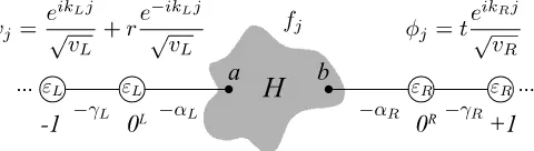


![Fig. 11. Generalized transport model using Green’s function method. Generalized transport model using equilibrium Green’s function method [28] and itsequivalent model for a simple 1D problem.](https://thumb-us.123doks.com/thumbv2/123dok_us/9347977.436837/18.612.104.508.59.555/generalized-transport-function-generalized-transport-equilibrium-function-itsequivalent.webp)
Related documents
Therefore, nonparametric effects of continuous covariates can be estimated on the basis of penalized splines, random walks or univariate Gaussian random fields priors (see
dir and ligand sequence number in the file macro.dir; (4) ligand molecular weight; (5) number of hydrogen- bond donors, acceptors, rotatable bonds, rings and NO 2 groups in the
Interplay of irreversible reactions and hydrofracturing This subsection derives reaction relations that formed the reaction zone between the serpentinite and rodingite, to explain
In this paper, we thus describe and discuss two methods to estimate parameters of LIF models with the added complexity of a time-varying input current. We assume that the
Students were grouped into experimental (6A class) 11 and control (6B class) 10. Equal number was not possible since the intact classes were used.. thereafter taught narrative
Although I maintain that values are either equivalent with constructs, or consistent with them at the very least, this claim in no way precludes individuality or uniqueness in one's
(A and C) Chorein immunoblotting results revealed reduced chorein immunoreactivity in the erythrocyte membranes of patients with MLS, which are equivalent to the heterozygous
The overall aim of this study was to inform the devel- opment of equitable and accessible mental healthcare integrated into primary care services for people with se- vere
