Feasibility study of a simulation software tool development for dynamic modelling and transient control of adiabatic compressed air energy storage with its electrical power system applications

warwick.ac.uk/lib-publications

Manuscript version: Author’s Accepted Manuscript

The version presented in WRAP is the author’s accepted manuscript and may differ from the

published version or Version of Record.

Persistent WRAP URL:

http://wrap.warwick.ac.uk/107917

How to cite:

Please refer to published version for the most recent bibliographic citation information.

If a published version is known of, the repository item page linked to above, will contain

details on accessing it.

Copyright and reuse:

The Warwick Research Archive Portal (WRAP) makes this work by researchers of the

University of Warwick available open access under the following conditions.

Copyright © and all moral rights to the version of the paper presented here belong to the

individual author(s) and/or other copyright owners. To the extent reasonable and

practicable the material made available in WRAP has been checked for eligibility before

being made available.

Copies of full items can be used for personal research or study, educational, or not-for-profit

purposes without prior permission or charge. Provided that the authors, title and full

bibliographic details are credited, a hyperlink and/or URL is given for the original metadata

page and the content is not changed in any way.

Publisher’s statement:

Please refer to the repository item page, publisher’s statement section, for further

information.

1 Introduction

Electrical Energy Storage (EES) has been recognized as one of the significant technologies for solving great challenges in modern power systems, e.g., the network’s reliability with a rapid increase of intermittent renewable

energy generation. Among all EES technologies, Pumped Hydroelectric Storage (PHS) is a technology with high technical maturity and large energy/power capacity, which dominates the worldwide EES bulk storage capacity [1,2].

Apart from PHS, Compressed Air Energy Storage (CAES) is another commercialized technology with bulk storage capacity, which can offer both technical and economic benefits in different stages of power networks (e.g. generation,

transmission, and distribution) with multi-scales (from a few kW to over 100 MW) [1,2]. It is proven that CAES has many outstanding advantages, such as large-scale availability, low operation cost, long lifetime and established

Feasibility study of a simulation software tool development for dynamic modelling and transient control of adiabatic compressed air energy storage with its

electrical power system applications

Xing Luoa

Mark Doonera

Wei Hec

Jihong Wanga, b, ⁎

[email protected], [email protected]

Yaowang Lib

Decai Lia

Oleh Kiselychnyka

a_{School of Engineering, University of Warwick, UK}

b_{School of Electrical & Electronic Engineering, Huazhong University of Science & Technology, China}

c_{Department of Mechanical Engineering, Massachusetts Institute of Technology, United States}

⁎_{Corresponding author at: School of Engineering, University of Warwick, UK.}

Abstract

The field of large-scale electrical energy storage is growing rapidly in both academia and industry, which has driven a fast increase in the research and development on adiabatic compressed air energy storage. The

significant challenge of adiabatic compressed air energy storage with its thermal energy storage is in the complexity of the system dynamic characteristics arising from the multi-physical (pneumatic, thermal, mechanical and

electrical) processes. This has led to a strong demand for simulation software tools specifically for dynamic modelling and transient control of relevant multi-scale components, subsystems and whole systems with different

configurations. The paper presents a feasibility study of a simulation tool development implemented by the University of Warwick Engineering team to achieve this purpose. The developed tool includes a range of validated

simulation models from the fields of pneumatics, thermodynamics, heat transfer, electrical machines and power grids. The structure of the developed tool is introduced and a component library is built up on the

Matlab/Simulink platform. The mathematical descriptions of key components are presented, which precedes a presentation of four case studies of different applications. The case studies demonstrate that the simulation

software tool can be used for dynamic modelling of multi-scale adiabatic compressed air energy storage components and systems, real performance analysis, dynamic control strategy implementation and feasibility studies of

applications of adiabatic compressed air energy storage integrated with power grids. The paper concludes that the continued development and use of such a tool is both feasible and valuable.

industrial experience [1,2].

The working principle of a conventional CAES plant can be described as follows. During the charging (compression) mode, the electrical energy from the grid is used to drive a multi-stage compressor unit to compress the air

into a storage reservoir. To improve the efficiency of the compression process, the compressor unit normally uses coolers to reduce the air temperature after each stage of compression [1,2]. Also, for large-scale CAES plants, only

underground salt cavens have practical commericialcommercial operation experience for the purpose of storing a large amount of compressed air [2,3]. During the discharging (expansion) mode, the stored compressed air with high

pressures is released, heated by fossil fuel combustion, and then expanded via a multi-stage turbine (or expander). Finally the electricity is generated by an electrical generator connected to the main shaft of the turbine. Two

large-scale conventional CAES plants are in commercial operation worldwide, that is, 290 MW/580 MWh German Huntorf CAES plant and 110 MW/2860 MWh US McIntosh CAES plant. Both of them use the combustion of natural gas to heat

compressed air for electricity generation [2,3].

With the development of technology, the concept of adiabatic CAES (i.e., a hybrid combination of CAES and Thermal Energy Storage (TES) without involving fossil fuel combustion), has received much attention. In a

conventional CAES plant, a large amount of heat generated from the charging (compression) mode is directly released to the atmosphere via the cooler operation, which is a waste of useful energy. Adiabatic CAES can store and reuse

this heat energy in the CAES discharging (expansion) mode for enhancing the compressed air energy with high temperature to generate electricity [4–6]. This concept increases the complexity of the whole system because the closed

loop of the heat transfer medium to TES (including heat exchange and thermal storage units) must have the capacities and the performance to match the requirements of the air compression/expansion units. The key features of

adiabatic CAES include: (1) improving the cycle efficiency of the overall system, i.e., the cycle efficiency of adiabatic CAES could be up to around 70%, compared to Huntorf (42%) and McIntosh (54%); (2) avoiding the use of fossil fuels

in CAES discharging (expansion) modes, which is a significant advantage over the conventional CAES plants [1,2].

Some demonstration plants using adiabatic CAES technology have recently been built or are under construction. A multi-stage regenerative 500 kW demonstration system (named “TICC-500”), designed jointly by Tsinghua

University, Institute of Physics and Chemistry of Chinese Academy of Science and China Electric Power Research Institute, had its trial interconnection with the Chinese power grid in 2014 [2]. A 1.5 MW supercritical adiabatic CAES

demonstration system designed by Institute of Engineering Thermophysics of Chinese Academy of Science with its academic and industrial partners has been operating for more than 3000 h since its first test, running from 2014 [2,7].

The compressed air in a part of the air circuit of the system is at its supercritical state and the system cycle efficiency can achieve about 55% [2,7]. Based on this experience, Institute of Engineering Thermophysics of Chinese Academy

of Science has leaded another project – the first 10 MW adiabatic CAES demonstration project in China, which has started its test running in 2017 [2]. In Germany, it was claimed that the world’s first large-scale adiabatic CAES project

named ADELE has been designed by RWE Power, General Electric, Zűblin and DLR [8]. The targets of the project are: (1) adiabatic CAES combining other individual energy sources (especially wind power) to achieve electrical energy

storage completely without CO2 emissions, with 70% cycle efficiency; (2) the project has planed to have a storage capacity of 360 MWh and a power output of 90 MW [8]. However, the project is currently on hold due to uncertain

business conditions [2].

Academic researchers have explored the concept of adiabatic CAES with a range of different research focuses, such as simulation modelling, efficiency analysis and configuration optimisation. Luo et al. presented an adiabatic

CAES system model with a time-dependent dynamic model for the compressed air storage and thermodynamic (steady state) models for other components in the system (compressors, expanders, valves and pumps) [9]. Liquid water

was used as a heat transfer medium and for heat storage. The paper also reported a system parametric study and optimised the system’s configuration [9]. Hartmann et al. studied the simulation analysis of different adiabatic CAES

plant configurations [6]. The models of compressors and turbines were based on the thermodynamic state equations of the polytropic and isentropic processes. The study concluded that the efficiency of the polytropic configuration was

about 60%, and 70% efficiency could reach when choosing the isentropic (ideal) configuration [6]. Guo et al. studied a similar mathematical model for adiabatic CAES [10]. A simulation study on the cycle efficiency and the energy

storage density was carried out [10]. Wolf and Budt presented a techno-economic analysis of a low-temperature adiabatic CAES system and a simple thermodynamic description of the system was employed [5]. The theoretical study

indicated that the cycle efficiency is in the range of 52–60% with wide-ranging part load capabilities [5]. Chen et al. presented an isobaric adiabatic CAES system, in which CO2 and its mixtures are used as the volatile fluids for

extending the system operation over a wide range of ambient temperatures [11]. The thermodynamic analysis, including exergy efficiency analysis and a parametric analysis, was evaluated based on the developed steady state model

[11]. Wang et al. experimentally studied a pilot CAES system with TES, which used water as the TES working medium and heat storage [12]. An average cycle efficiency of 22.6% was achieved in the tests [12]. The paper discussed the

reasons for such a low efficiency: (1) the unsteady operation of the compressor caused by the pressure variation in the storage tank; (2) the output electric generator operating at its off-design conditions; (3) the non-optimal

performance of the TES subsystem [12]. These findings show the importance of dynamic control strategy development and implementation using a complete system (electricity-to-electricity) dynamic model for improving the cycle

efficiency. Peng et al. studied the thermodynamic performance of an adiabatic CAES system with a Packed Bed Thermal Energy Storage (PBTES) subsystem [4]. The thermal behaviour of PBTES was studied and then an updated

A-CAES system with a heat recuperator was further proposed to improve the cycle efficiency. An exergy analysis performed by Barbour et al. indicated that the main losses for adiabatic A-CAES with PBTES occur in the compressors and

expanders [13]. Both papers ([4,13]) focused on the dynamic modelling of PBTES. In Sciacovelli et al.’s model [14] (except for the compressed air reservoirs and PBTES) the compressors, turbines and heat exchangers used steady state

study linked the component performance and the plant performance, no electrical modelling (e.g. electric motors/generators/loads) was considered [14]. He et al. studied a cycle-to-cycle modelling framework to simulate adiabatic

CAES with PBTES [15]. Phase Change Material (PCM) filled PBTES and rock filled PBTES were studied respectively. The paper mainly focused on the study of thermodynamic variables (e.g., pressure, flow rate and temperature) and

the cycle efficiency analysis, while most mechanical and electrical variables (e.g., compressor torque and generator voltage/current) were not discussed. Tola et al. proposed a system configuration including axial compressors, radial

and axial turbines and a PBTES subsystem [16]. The article only presented a simple PBTES mathematical model. A simulation study including a cycle efficiency analysis was carried out, considering the off-design working conditions

[16]. In addition, a few overview papers focused on CAES technology development were recently published [2,17–19], and all of them have introduced the adiabatic CAES concept and its state of the art.

From the above research papers (i.e., [4–6,9–16], almost all of the modelling approaches used one or more thermodynamic (steady state) submodels (e.g., the submodels of compressors and expanders/turbines), and none

considered detailed submodels of relevant electrical components in the whole system. A complete dynamic system model should have time-dependent dynamic submodels of its all components. Additionally, there is no complete (i.e.,

electricity-to-electricity) time-dependent dynamic adiabatic CAES system model considering all involved multi physical (i.e., pneumatic, thermal, mechanical and electrical) processes. Thus the published modelling methods cannot

achieve full dynamic behaviors of the actual adiabatic CAES system. The dynamic performance can significantly differ from the steady state characteristics and consequently, dynamic control strategy development for the charging

(electricity-to-air) and discharging (air-to-electricity) processes, and the simulation studies of time-dependent power system applications (especially to the Grid Code realization and grid-connection applications), cannot be

implemented.

Although many efforts have been made, some significant challenges still exist, e.g., (1) both CAES and TES are complex systems with subsystem coupling, component interaction and parameter sensitivity, which require

time-dependent dynamic simulation studies; (2) the cycle efficiency of CAES within the wide working conditions depend on both system dynamic and static behaviours; (3) dynamic modelling of complete adiabatic CAES systems is essential

to provide support for feasibility studies of EES applications, system optimisation and control strategy development, and management of grid integration.

There is simulation software for power system modelling with different priorities, for instance, power system analysis for steady and dynamic states (e.g. DIgSLENT, PSS/E), electromagnetic transient (e.g. EMTP-RV, PSCAD),

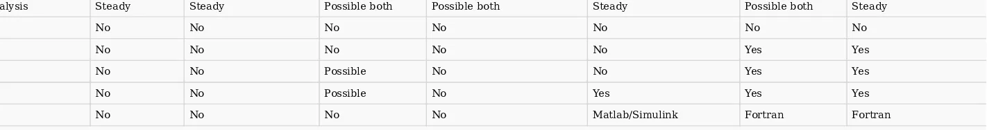
real-time simulation (e.g. OPAL-RT, dSPACE) and multi-physics analysis (e.g. Matlab/Simulink, DYMOLA) [20,21]. A comparison of the characteristics of available software with EES modelling capabilities is shown in Table 1. Although it

is not claimed that Thermolib includes EES modelling in its scope (refer to [22]), from Table 1 it can be seen that Thermolib is the only simulation software in which thermodynamic (steady state) modelling of CAES and TES could be

achieved. Thus, compared to the well-developed power system software available, the capabilities of software for EES simulation are limited. From the investigation presented in Table 1 and the literature review, it can be concluded

that there is a lack of appropriate simulation tools to (1) study the time-dependent dynamic performance of adiabatic CAES with consideration of the dynamic electricity usage/generation, (2) implement the essential dynamic controls

in the whole system or in the pneumatic, thermal, mechanical and electrical subsystems and (3) perform feasibility studies of adiabatic CAES in time-dependent power grid applications. Considering that the field of large-scale EES is

growing rapidly, there is a strong demand for the development of a specific simulation software tool for this purpose. Developing such a simulation tool faces great challenges, such as (1) a wide range of dynamic time-scales in

pneumatics (minutes), heat conduction (minutes), machinery (seconds to minutes) and electricity (milliseconds to seconds), causes the complete systems to be stiff and thus difficult to simulate; (2) interdisciplinary research in

pneumatics, thermodynamics, heat transfer, machinery and electricity adds integration challenges; (3) air compressibility, heat transfer complexity and strong non-linearity of components introduce difficulties in dynamic simulation; (4)

realization of such a tool creates logistical challenges, such as solving module standardization and coding problems (e.g. model coupling, algebraic loops).

Table 1 A comparison of simulation software with EES modelling capabilities [22–28].

Function Software

Homer Energy Plus Power

world Energy 2020 Thermolib AspenPlus Protrax

Economic/

technical study Both Both Both Mainly on economics Technical analysis Both Technical analysis

EES pertinence Yes Yes Yes Yes Indirect

(no claim) No No

Types of EES technologies Flywheels,

battery, hydrogen

TES Battery Pumped hydro,

fuel cell Possible TES, CAES N/A N/A

Round-trip efficiency Yes No No Yes N/A N/A N/A

Steady/dynamic state analysis Steady Steady Possible both Possible both Steady Possible both Steady

Multi-physics analysis No No No No No No No

Real-time simulation No No No No No Yes Yes

Dynamic control No No Possible No No Yes Yes

User defined function No No Possible No Yes Yes Yes

Co-simulation No No No No Matlab/Simulink Fortran Fortran

Considering the above, development of a specific simulation software tool for multi-scale adiabatic CAES is proposed. The features of this simulation tool include: (1) it is the first simulation software software tool specifically

for dynamic modelling and transient control of adiabatic CAES; (2) it consists of a range of complex and novel time-dependent dynamic models and thus many components’ and systems’ variables can be simulated, many of which are

not available in the steady state models, e.g., the time-dependent dynamic shaft rotation speeds of compressors and expanders; (3) the adiabatic CAES charging and discharging processes can be dynamically controlled using the

developed simulation tool (e.g., pneumatic regulators and valves can be controlled in time series like their real counterparts; the electric motor driving the compressor and the electrical generator driven by the expander can be also

dynamically controlled); (4) the developed simulation tool sets up a bridge from the CAES and TES technologies themselves, to the electricity generation and the power grid, which can be directly used for the feasibility studies of

power grid applications, e.g., grid frequency and voltage controls (which essentially require the transient analysis of the integration of EES systems onto power grids); (5) the initial version of the developed tool is currently under

internal tests on a server (refer to https://estoolbox.org/), and it will be open source and will thus facilitate and support research projects in the relevant EES with power grid application areas. A feasibility study to evaluate the

potential development and use of the tool is presented in the paper. Four case studies using the initial version of the developed tool are also presented, which indicate that the proposed tool can provide important support for adiabatic

CAES research and development and its grid application study.

2 Structure of the proposed simulation software tool

To implement the simulation tool, the component-based modular design method is chosen, which enables the construction of complicated systems to be easily carried out. The characteristics of this simulation tool will be: (1)

based on the established component library, the user is able to easily assemble the ready-to-use components together to model the whole system; (2) user-defined models can be linked with the pre-developed component library models;

(3) a component model is able to stand for its real counterpart, and the model can show the same behaviours as its counterpart in real systems; (4) the structures of the component models across the entire simulation software tool are

standardized (including the input/output variables, the parameter settings and the initial condition settings), to allow for ease of use and integration of all components. Fig. 1 illustrates the structure and connection of the component

models in the simulation software tool, which shows their external characteristics, settings and relationships with other component models. It can be seen that the input variables of a component model can be the outputs of the

upstream model(s) and/or the feedback from the downstream model(s). In some cases, there are special items in the settings or modelling processes (see Fig. 1), which need to be carefully considered, such as a moment of inertia of a

system, especially when the shafts of two or more components are coupled together in the system.

Fig. 2 shows the library of the proposed simulation software tool. The multi-level classification method has been used. Fig. 2(a) presents the library structure of the proposed simulation software tool. Fig. 2(b) shows the top

level of the library implemented in the Matlab/Simulink platform. For the top level, the first eight categories (“1–8” in Fig. 2(a)) are classified based on their physical functions; the last (“9” in Fig. 2(a)) gives simulation examples for

case studies. For the second level, the classification is based on the different approaches of mathematical modelling (e.g. modelling for thermodynamic steady state analysis and modelling for dynamic simulation & control, “10–17” in

Fig. 2(a)) or the functions of machines (e.g. “18–20” in Fig. 2(a)). The second level subdirectory can continually divide into the third level subdirectory and so on. The high number of component models can be clearly sorted by the

logical multi-level structure of the library, and the required components can be easily located by the user when building complex system models. In addition, with such a structure, it is easy to extend the library, e.g. the subdirectories

of “measurements” and “pneumatic actuators” can be added if needed (see Fig. 2).

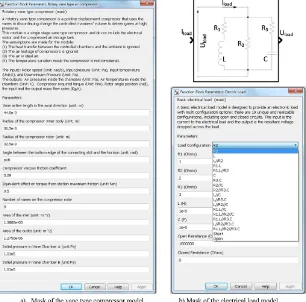
Each model must clearly show its inputs and outputs, parameter settings and initial conditions. Fig. 3 shows two typical examples of component model masks. It can be seen that the model mask for the vane type compressor

model has a brief introduction, the parameter settings for its geometrical structure and its friction coefficients, and the initial conditions of chamber pressures (Fig. 3(a)). Apart from the parameter settings, the model mask for the

individual model is accompanied by a document giving details of its physical counterpart, modelling assumptions and equations, and detailed parameter and I/O information.

3 Mathematical modelling of key adiabatic CAES components

In this section, the modelling descriptions of some typical adiabatic CAES components (including compressors, turbines, heat exchangers, storage reservoirs, electrical generators/motors and loads) implemented in the

simulation tool are presented. In order that the reader can follow a linear and effective path along the article scope, the detailed mathematical equations for the modelling of the described components are given in Appendix A.

3.1 Compressors

For the mathematical modelling of compressors, the modelling approach for thermodynamic (steady state) analysis (“10” in Fig. 2(a)) has been widely used and it can be summarized as follows: (1) the compression process is

assumed to be an isentropic, isothermal or polytropic thermodynamic process; (2) the equations of states are used to calculate the state variables (e.g. pressures and temperatures); (3) an actual output is calculated based on the

assumed thermodynamic process with introducing a corresponding efficiency (e.g. isentropic efficiency). A typical example can be found in [9]. However, such a method can only be used for steady state analyses because dynamic time

dependent processes are not modelled.

Regarding to dynamic modelling and transient control of compressors, the modelling approach for positive displacement compressors (e.g. piston, vane, screw and scroll types) is described in this section, which is illustrated in

Fig. 4: (1) the compressor chamber volumes with their time-based change rates are derived from the compressor geometric structures; (2) the differential expressions describing the chambers’ pressures and temperatures are derived

In this paper, the dynamic modelling of piston compressors is used as an example. The piston machine, as a mature technology [2,29], can be used in small/middle-scale CAES. The detailed mathematical equations for the

dynamic modelling of this type of compressor is described in Appendix A.

3.2 Turbines and expanders

For the category of turbines and expanders, the modelling method for thermodynamic (steady state) analysis (“16” in Fig. 2(a)) is similar to the modelling approach described in the first paragraph of Section 3.1. Also, the

method for dynamic modelling of positive displacement expanders (“17” in Fig. 2(a), e.g. piston type) is similar to the approach illustrated in Fig. 4. An example of dynamic modelling for scroll expanders was reported in the authors’

paper [30].

In addition, the working principle of turbomachinery (e.g. radial turbines) differs from that of positive displacement machines: turbomachinery converts energy between the rotational kinetic energy of the impeller and the

dynamic energy of the fluids, while positive displacement machines uses controlled chambers with variable dimensions to complete compression or expansion processes. Thus, a specific modelling methodology for turbomachinery is

required. Based on the above, a numerical model for radial turbines is presented in Appendix A, which can be connected dynamic models of electrical generators to simulate the dynamic performance of radial turbines.

3.3 Compressed air storage reservoirs

Similar to the modelling of compressors and turbines/expanders, two types of modelling approaches (“12” and “13” in Fig. 2(a)) are considered in the simulation tool. There are three types of natural geological options which

have the possibility to be used for scale CAES, including salt caverns (in bedded or domal salts), hard rock and porous rock. To date, only the caverns constructed in salt domes have practical experience for commercialized

large-scale CAES [1,2]. The air storage in the caverns made from salt domes have been used in both Huntorf and McIntosh CAES plants. Thus, the dynamic modelling of salt caverns is presented in Appendix A.

3.4 Heat exchangers and thermal storage

The Heat Exchanger (HEX) is an essential component of adiabatic CAES systems. Effective HEX design can improve the whole system performance, especially to enhance the thermal energy reuse for the CAES discharging

process and in turn to increase the whole system cycle efficiency. In the 1.5 MW demonstration system operating at the Institute of Engineering Thermophysics of Chinese Academy of Science, the tube and shell type of HEXs have been

used and liquid water is chosen as the working medium for heat transfer and storage [2,7]. In the initial version of the developed simulation tool, both the steady state and the dynamic models for such type of HEX are available, and

their mathematical equations are presented in Appendix A.

Based on the range of operating temperature, thermal storage can be classified into two groups: low-temperature (e.g. aquiferous TES) and high-temperature (e.g. latent heat TES). The water tank has been widely used as a

heat storage reservoir, e.g., the 1.5 MW advanced adiabatic CAES demonstration system in China [7]. In the initial version of the developed tool, the model for water tanks (i.e., a major component used for low-temperature thermal

storage) is available, which is briefly described in Appendix A.

3.5 Electrical power systems

Modelling of the electrical subsystems is important to the CAES system modelling; however, the published papers did not take this into serious consideration. This section introduces the dynamic models for AC synchronous and

asynchronous machines, a utility electrical load model with resistance, capacitance and inductance combined, and a frequency response model for adiabatic CAES implemented in relevant grid applications.

3.5.1 Synchronous and asynchronous electrical machines

At present, many thermal power plants, hydropower plants and nuclear power plants use synchronous generators for electricity generation; and the power factor of non-permanent magnet (non-PM) synchronous generators can be adjusted by

generators in the rotor d-q reference frame is briefly described in Appendix A.

Three-phase asynchronous motors have been widely used in industry because they are reliable, robust and economical [31–33]. With proper motor drives, they can offer good energy saving opportunities in variable torque/frequency applications

[31,32]. Thus, the asynchronous motor can be used for CAES operation in the charging mode. The dynamic model for asynchronous motors in the d-q reference frame is available in the developed simulation tool, and is described in Appendix A.

3.5.2 Electrical load

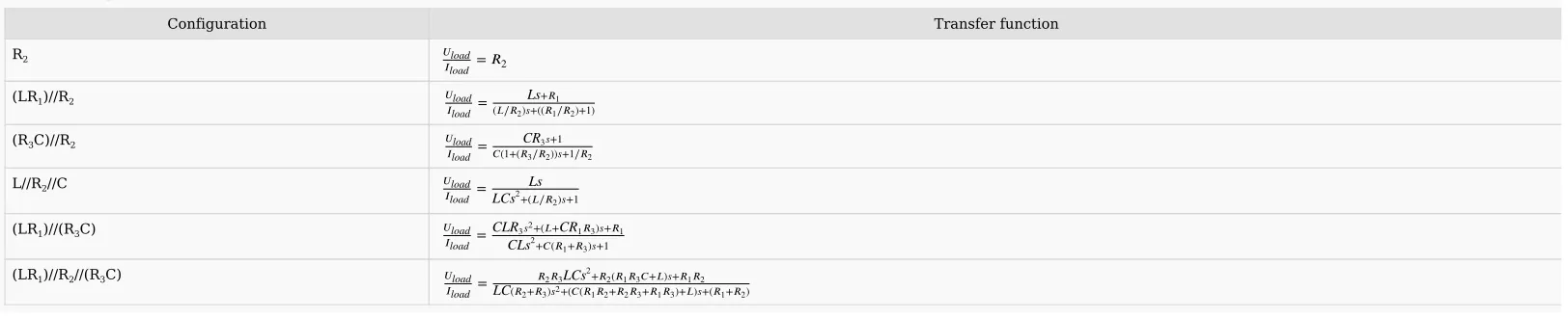
A utility electrical load model is designed to provide an electronic load with multiple configuration options. The represented circuit of the electrical load model is given in Fig. 3(b). The input and the output of the model are the load current ( )

and the load voltage ( ), respectively. The resistors (R1, R2, R3) can take the state zero (i.e., a short circuit), infinity (i.e., an open circuit) and present (i.e., the component is present and requires a positive value); the inductor L and the capacitor C can

take the state zero and present. Considering the different states of each of the five components (R1, R2, R3, L and C in Fig. 3(b)), a range of configurations can be modelled, that is, 19 unique and realizable configurations in total. The transfer functions of

six examples of configurations are listed in Table 2 shown in the corresponding section of Appendix A. The model integrated with the generator model forms a loop circuit, which can be used for electrical power system simulation.

3.5.3 Grid frequency response

For the utility power system, its frequency must be controlled within a very tight range due to the electricity usage regulation (named Grid Code), e.g. the normal operation frequency variation intervals are within for the U.K. grid [34].

Disturbances in the power system can cause a frequency deviation from its rated value. For instance, because the rotation speed of the synchronous generator in the power plant is synchronic to the grid frequency, the frequency will be raised when the

input shaft power of the synchronous generator exceeds the power of load demand. Frequency regulating units in the power system must take action in such a situation. EES can be used for frequency response control service to the electrical power

system.

The developed model in the tool can be used to simulate the grid frequency response with the electrical system power balance variation. The model can be applied to the study of grid frequency response with EES operation for power system

frequency stabilization. A case study is given in Section 4. The mathematical equations for this model are introduced in the corresponding section of Appendix A.

4 Application case study of the simulation software tool

Both the models for thermodynamic analysis and the models for dynamic simulation can be used for the analysis of steady state performance and the feasibility study of system configuration. The authors’ recent research paper

[9] shows an example for such purposes. The paper presents a complete adiabatic CAES system model for steady state analysis (refer to [9]). The developed dynamic models in the simulation tool have additional features due to the

capabilities of dynamic simulation which allow for other types of analyses and studies to be carried out. This section presents four application case studies using the dynamic models in the developed tool, in the areas of model

validation, dynamic simulation of the whole system, transient control of adiabatic CAES components and systems, and grid frequency service.

4.1 Models validation

The dynamic model can show the same transient behaviours of the real systems they represent. The validation can be carried out through comparing the open-loop responses from the experimental data (or the reference data)

and the simulated results of the corresponding model. In this section, graphical comparisons in figures (Figs. 5–7) and Mean Relative Error (MRE) are chosen for quantitative analysis. MRE can be defined as,

where is the number of samples; stands for the data from the actual measurements of the real components/systems (or reference data); represents the data from the simulation results of the corresponding

models. In this section, the validation for piston compressors, salt caverns and radial turbines are presented as examples.

Iload

Uload

(1)

A two-stage reciprocating compressor (BroomWade, type: TS9-16) with its experimental test data described in [35] is used for the piston compressor model validation. The used parameters are given in Table 3 which refers to

Table A1 in [35]. The unknown parameters can be identified using a Genetic Algorithm with the experimental data (refer to [38]). The crankshaft speed of the compressor is 425 rpm as a constant input to the model. The initial air

pressures and air temperatures in the low pressure and high pressure cylinders are  Pa and 293 K respectively. Fig. 5 shows the comparisons of experimental and simulated air pressures within one complete cycle (i.e., crank

angle from 0° to 360°) in the two cylinders. It can be seen that the experimental and simulated air pressures in both cylinders roughly agree with each other. However, differences between the experimental data and the simulation

results can be in Fig. 5 and thus the MRE has been studied: the MRE of the air pressure in the low pressure cylinder is 0.079; the MRE of the air pressure in the high pressure cylinder is 0.084. The MRE can be reduced by detailed

modelling of the cylinder inlet and outlet valves, which have been simplified in the current modelling process.

Table 3 The parameters of the compressor for model validation [35].

Parameters Value

Number of cylinders 2

Compressor crank shaft speed (rpm) 425

Stroke lengths for both cylinders (m)

Connecting rod lengths for both cylinders (m)

Fig. 5 Model validation for the developed piston compressor dynamic model (experimental data from [35]).

Fig. 6 Model validation for the salt cavern dynamic model (referenced data from [3,36]).

Fig. 7 Model validation for the radial turbine model (experimental data from [37]).

1.011×105

7.62×10 - 2

Crank radius for both cylinders (m)

Low pressure cylinder bore (m)

High pressure cylinder bore (m)

Maximum inlet valve lift (m)

Maximum discharging valve lift (m)

Low pressure cylinder

’

High pressure cylinder

’

The experimental data of air pressure inside the salt cavern of the Huntorf CAES plant (refer to [3,36]) is employed for the salt cavern model validation. The simulated result of the air temperature within the salt cavern in [3] is

also used in this paper for simulation comparison. The parameters are given in Table 4. The input and output mass flow rates of the salt cavern shown in Fig. 6(a) and (b) are used as the model inputs via the method of lookup tables. The

initial air pressure and temperature inside the salt cavern set at  Pa and 330 K respectively. Fig. 6 shows the comparison of experimental and simulated air pressures, and the comparison of simulated air temperatures,

respectively. From Fig. 6, it can be seen that the data of air pressures and temperatures are well matched. The MRE of the cavern pressure based on the data given in Fig. 6(c) is 0.009, and the MRE of the cavern temperature

calculated from the data shown in Fig. 6(d) is 0.003.

Table 4 The parameters of the salt cavern used for model validation [3].

Parameters Value

Volume of the cavern storage (m3_{) 300,000}

Cavern operating pressure (Pa) to

Maximum cavern pressure (Pa)

Maximum discharge rate (Pa/hour)

Cavern wall temperature (K) 323

Natural convection heat transfer coefficient 0.2356

Forced convection heat transfer coefficient 0.0149

The experiment-based isentropic efficiency of a turbine presented in [37] is used for the radial turbine model validation. Table 5 lists the parameters of the radial turbine described in [37]. The input rotor rotation speed and the

pressure ratio of ( and are air pressures at the stator nozzle and at the rotor exit, respectively) are set to be variables for obtaining the isentropic efficiencies at different conditions. The isentropic efficiency of the

turbine can be defined as [39,40],

3.81×10 - 2

9.36×10 - 2

5.55×10 - 2

2.2×10 - 3

2.6×10 - 3

1.25×10 - 2

1.05×10 - 2

48.6×105

46×105 66×105

72×105

10×105

PTair3/PTair1 PTair1 PTair3

where is the rotation speed of radial turbine in rad/s; is the enthalpy change of air from turbine inlet to outlet with the assumption that the air through the turbine is an ideal isentropic process; and are the

two parts of the torque generated on the rotor, i.e., obtained from the sudden deflection of the flow when entering the rotor and developed in the rotor passage; and are tangential velocities of the rotor at its

inlet and outlet, respectively; and are the tangential velocities of air at the rotor inlet and outlet; is universal gas constant; is the ratio of specific heats; is air temperature at the stator nozzle inlet; is the

stator nozzle outlet angle; is the rotor exit angle.

Table 5 The parameters of the radial turbine used for model validation (Figs. 4 and 9 in [37]).

Parameters Value

Diameter of rotor periphery (diameter of rotor at inlet) (m) 0.1164

Mean diameter of rotor exit (m) 0.0520

Depth of rotor entry section (m) 0.0063

Depth of rotor exit section (m) 0.0216

Rotor inlet angle from mean velocity triangle (degree) 77.6

Rotor exit angle from mean velocity triangle (degree) 57.4

Fig. 7 shows the comparison of experimental data and simulation results for the isentropic efficiency of a radial turbine (the experimental data is from [37]). For the data comparison with the reference [37], the ratio of the rotor

peripheral velocity ( ) and the stage terminal velocity ( ) is used here (i.e., as the x axis of Fig. 7). From Fig. 7, when the pressure ratios of are at 4 and 5 respectively, the corresponding MREs are 0.008 and 0.006

individually. The comparisons approximately agree and thus the model for radial turbines is validated.

The validated models can represent the dynamic performances of the real counterparts and can thus be used in practical control design, model based control strategies, hardware-in-the-loop experiments, system design, system

and component optimization, efficiency analysis and parameter sensitivity studies. AdditionalyAdditionally, due to the non-linear characteristics of most CAES components, the validated models can be used to find their approximation in

the form of a Fourier series expansion for applying advanced control theory.

4.2 A MW scale adiabatic CAES system dynamic simulation

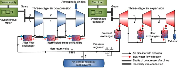
The simulation study of the dynamic modelling of a complete cycle (electricity-to-electricity) of a MW scale adiabatic CAES system is presented. Fig. 8 shows the whole system layout. An asynchronous motor with a three-stage

piston compressor and a synchronous generator with a three-stage radial turbine are used in the CAES charging and discharging modes, respectively. A salt cavern is chosen for compressed air storage. An ideal three-phase electricity

supply (rated phase voltage 220 V and rated frequency 50 Hz) is used to power the asynchronous motor. A non-return valve and a pressure regulator, as auxiliary components, are employed for air flow and pressure control purpose (see

Fig. 8). The main parameters used for the simulation study are listed in Table 6 (considering the length of Table 6, it is presented in Appendix B).

ωT Δhin→out,s τT1 τT2

τT1 τT2 veTrotor2 veTrotor3

γ TTair1 α2

α3

vTrotor2 cst PTair1/PTair3

An adiabatic CAES system was recently studied by the authors in [9], which uses liquid water for heat transfer and storage. For the study, considering the complexity of the whole system and with a view to saving computer

memory for simulation, the HEX and the water thermal storage with the same structure in [9] are used. The HEX effect on air temperatures in the charging and discharging modes has been assumed based on the system numerical

analysis in [9]. It is assumed that: after the three HEXs in the air compression mode (the blue circular points in Fig. 8(a)), the air temperatures drop to 310 K; after three HEXs in the air expansion mode (the red circular points in Fig.

8(a)), the air temperatures increase to 370 K. The simulation study of such type of HEX will be presented in Section 4.4 and the above assumptions also approximately match the simulated results given in Section 4.4 (the air

temperature at its steady state shown in Fig. 13(a)).

Fig. 9 shows the simulation results for the case study, including dynamic responses of the piston compressor crankshaft rotation speed (Fig. 9(a)), the air pressures inside three cylinders of the piston compressor (Fig. 9(b)), the

air temperature and pressure inside the salt cavern in a complete charging-storage-discharging cycle ((Fig. 9(c) and (d)), the air pressures before and after the pressure regulator in CAES discharging (Fig. 9(e)), the isentropic efficiency

of the 3rd stage radial turbine during CAES discharging (Fig. 9(f)), the mass flow rate of the radial turbine with its generated mechanical torque (Fig. 9(g)) and the rotation speed of the synchronous generator with its electrical load

From Fig. 9, it is seen that, via using the dynamic models in the developed tool, the real dynamic performance of components with variables can be simulated, such as the rotation speeds of machine shafts (Fig. 9(a) and (h)) and

the air pressures/temperatures inside cylinders/caverns (Fig. 9(b), (c) and –(d)). From Fig. 9, the CAES charging process takes approximately 4.66 h and the air pressure inside the salt cavern increases from  Pa to  Pa. The CAES storage process takes 8 h, and both air pressure and air temperature in the salt cavern slightly reduce due to heat loss. The CAES discharging process takes approximately 0.6 h and the air pressure inside the cavern returns to

around  Pa. . From the consumed and generated electrical powers during the charging and discharging processes with their duration time, the electricity-to-electricity cycle efficiency can be obtained as around 58.9%. Fig. 9(a)

shows that the compressor speed is maintained at around 500 rpm in its steady status with some small vibrations because of the compressor’s mechanical torque variation in cycle-to-cycle operation. The functionality of the pressure

regulator is clearly shown in Fig. 9(e), i.e., maintain the regulator output pressure to match a given pressure reference (e.g., set at  Pa in this case study) until the regulator input pressure is lower than this pressure reference.

With the pressure regulator operation, if the turbine’s load (i.e., the electrical generator with its load) remains constant, the turbine’s mechanical torque generated from compressed air power can be dynamically controlled. Also, Fig.

9(g) and (h) shows the variations following the pressure regulator output change, such as the mass flow rate of the turbine dropping from 5.5 kg/s to 4.5 kg/s. Fig. 9 Simulation results of a complete cycle of a MW scale adiabatic CAES system.

4.6×106 6.5×106

4.6×106

It can be seen that, from the subsystem/system level, the dynamic model can capture many more system variables (e.g., the rotation speed of compressor rotors), especially their transient variations (e.g., the air temperature

variation inside the salt caverns), compared to the thermodynamic (steady state) models. The dynamic model for adiabatic CAES systems can be used for the study of the interactions between the components/subsystems,

subsystem/system level efficiency analysis, system parametric studies, dynamic control strategy implementation and system optimisation. Its powerful simulation capacity can be also used as a guide for implementing a new

demonstration system.

4.3 The charging process of a kW scale CAES system with dynamic control

Nowadays the small-scale CAES technology attracts much attention due to its merits, e.g., environmentally friendly and low maintenance cost. Considering that small-scale CAES normally has a faster response than large-scale

CAES, it requires a proper process control for its operation at the desired conditions. Also, small-scale CAES normally uses air tanks for storing compressed air with a wide pressure range (up to a few hundreds of times of the

atmospheric pressure), which causes the requirement for efficient control of the relevant electrical machine. This section shows a simulation study of the charging process of a kW scale adiabatic CAES system with dynamic cascade

control.

Here the configuration layout of the simulated small-scale CAES charging system is similar to the compression of the MW scale adiabatic CAES system presented in Section 4.2, i.e., a three-stage piston compressor with three

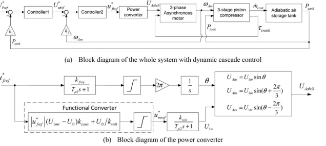
HEXs. Fig. 10(a) illustrates the block diagram of the whole system with the proposed cascade control strategy. An adiabatic air tank is employed for storing compressed air. Table 7 lists the main parameters used in this case study

(considering the length of Table 7, it is presented in Appendix B). From Fig. 10(a), it is seen that there are two coupling relationships leading to the system complexity: (1) the asynchronous motor coupling with the piston compressor via

the motor rotor speed ( ) and the compressor required torque ( ); (2) the piston compressor coupling with the adiabatic air tank via the compressor output mass flow rate ( ) and the air pressure inside the storage tank (

). Because an adiabatic air tank is used, the effective heat transfer coefficient . A power converter (also named frequency converter for controlling AC machines) replaces the ideal three-phase electricity supply shown in

Fig. 8 for control purpose (Fig. 10(a)).

For such a small-scale adiabatic CAES charging system shown in Fig. 10(a), safe and efficient regulation of the tank pressure is necessary. This requires automatic smooth motor start-up and stopping when the pressure reaches

the desired level. Also, to improve the efficiency of the motor, its speed during pressure transients should be kept at a rated value. Thus, a cascade control strategy as shown in Fig. 10(a) with different control methods can be

implemented. The internal loop control should be faster than the external loop control. Here the internal control is the motor speed control and the external control is the storage tank pressure control.

For instance, PID control is used in Controller 1 and 2 respectively (Fig. 10(a)). The control signal generated from the PID controller is: , where is the tracking error; are the

proportional, integral and derivative gains. In Controller 1 (i.e., the external control), is the difference between the reference corresponding to the target pressure ( ) and the dynamic pressure inside the tank ( )

multiplied by a feedback gain ( ); the signal generated from Controller 1 is the reference corresponding to the asynchronous motor rotor speed ( ). In Controller 2 (i.e., the internal control), is the difference between the

reference ( ) and the speed of the asynchronous motor rotor ( ) multiplied by a feedback gain ( ); the output signal of Controller 2 is the reference corresponding to the power converter frequency ( ).

The power converters used for the AC machine control indicate intermediate conversions of AC-DC and/or DC-AC voltages, to achieve the regulation of frequency and voltage magnitude of the AC machine power supply. The

ωAm τcrank

Ptank χtank,heat≈0

Fig. 10 a small-scale adiabatic CAES charging system with dynamic cascade control.

kp,kI,kD

Ptank

k1

transient mathematical descriptions of power converters can be approximated by aperiodic functions as shown in Fig. 10(b). It is seen that: one channel is for frequency regulation with the reference , the channel gain and the

time constant ; another channel is for voltage magnitude regulation with the reference , the gain and the time constant . The functional converter (Fig. 10(b)) sets a specific relationship between the frequency

channel reference and the voltage magnitude channel reference , where , is the rated frequency. The output signal of the power converter contains three stator phase voltages.

Fig. 11 shows the simulation results for this example study, including the dynamic response of the required mechanical torque of the three stage piston compressor (Fig. 11(a)), the comparison of the asynchronous motor rotor

speeds with and without the proposed control (Fig. 11(b)), the output signals of the two controllers respectively (Fig. 11(c) and (d)), the transient process of the voltage magnitude ( ) of the power converter (Fig. 11(e)), and the

variations of air temperature and pressure inside the adiabatic air tank with the control (Fig. 11(f)). From the simulation results, it is clearly seen that: (i) with the operation of controllers, the motor rotor speed can be well controlled,

to provide a smoother start-up process of the motor compared to the scenario without control (Fig. 11(b) and to maintain the speed at a desired value when necessary (Fig. 11(b)); (ii) the required compressor mechanical torque has

some oscillation due to the cycle-to-cycle variation of cylinder pressures, and the average torque is gradually increased from 6.5 N m to 32.8 N m resulting from the rising of the downstream tank pressure (Fig. 11(a)); (iii) the maximum

tank pressure (  Pa, Fig. 11(f)) and the stopping action of the compressor can be managed well via the dynamic control; (iv) the voltage magnitude ( ) from the power converter varies with the frequency regulation reference (

) (Fig. 11(d) and (e)).

In summary, from the simulation study, the functionality of using the developed software tool for dynamic control of the charging process (electricity-to-air) is presented and discussed. Based on this, the application can be also

implemented in the (advanced) control of the discharging process (air-to-electricity), the thermal storage subsystem and the whole adiabatic CAES cycle process. Considering that the dynamic models can reflect the real system

behaviours, the application areas can involve the practical control engineering implementation and Rapid Control Prototyping (RCP) of the relevant CAES with TES subsystems/systems.

4.4 Electrical energy storage servicing grid frequency control

kfreq

Tμ1 U1m kvolt Tμ2

fr UAabcS

U1m

2.5×106 U1m

A simulation study of a hybrid EES system servicing grid frequency control is presented here. The study focuses on the grid primary frequency control which should be able to stabilize the grid frequency to a steady state value

(but it normally cannot let the grid frequency return to its rated value) [34,41]. Based on the Great Britain (GB) Grid Code, the requirement of primary frequency control is the minimum increase in active power output within the

duration of 10–30 s after the time of the start of frequency fall [34]. From the review, the response time (standby to full power) of the 110 MW McIntosh plant and the 290 MW Huntorf CAES plant is 5–12 min [41]. From this, large-scale

CAES technology alone is not suitable for primary frequency control. But if it integrates with fast response EES technologies (e.g., batteries and flywheels) for power quality, the whole EES system can be used for such services. In the

simulation study, the total mass flow rate of pressurized water (as heat transfer fluid) flowing into the heat exchangers is set at 6.4 kg/s with the temperature at 393 K.

Fig. 12 shows the system layout for the simulation study. An adiabatic CAES discharging subsystem (2 MW) is implemented. The conditioning unit is for regulating/converting AC or DC electricity to match the grid connection

requirements. The parameters of the models of the synchronous generator and the three-stage radial turbine are the same as in Table 6. The parameters to the HEX and the grid frequency response models are listed in Table 8. The

parameters relevant to the grid frequency response model are guided by the UK power grid regulation (refer to [42]).

Table 8 The parameters of the simulation study in Section 4.4.

Parameters Value

Type of flow directions of HEX Counter flow

Heat transfer coefficient of HEX (W/(m2

Effective heat transfer area inside one HEX (m2_{) 150}

Initial temperature of air inside the HEX (K) 280

Initial temperature of water inside the HEX (K) 373

Power grid droop characteristic (Hz/MW) 0.04

Power grid inertia constant (sec) 10.8

Power grid damping factor 1

Grid rated frequency (Hz) 50

Electrical energy storage rated power capacity (MW) 2

Grid rated power capacity (MW) 200

Fig. 13 shows the simulation results of this example study, including the dynamic responses of air temperatures at the inlet and outlet of the last HEX (the HEX prior to the 3rd stage turbine, see Fig. 12), the CAES with TES

system electrical power generation, and the grid frequency responses. In the simulation, the load demand in the large power grid system (200 MW grid capacity) has a step increase (i.e., 4 MW increase) from its rated condition at the

simulation time of 10 s, which leads to the grid frequency fall (Fig. 13). Three scenarios have been considered at the moment of the grid frequency fall: (i) without any extra action being taken, i.e., there is no EES system used); (ii) the

responses of the three scenarios are simulated as shown in Fig. 13(c). It is clear to see that, the primary frequency control has a better performance when using a hybrid CAES with TES plus instantaneous response EES facility

compared to the other scenarios, because the grid frequency has a smaller variation during its transient process and can achieve quicker stabilization at a steady state value (Fig. 13(c)). Also, it can be observed that the quality of

primary frequency control highly depends on the response time of the increase in active power injection into the power grid system after the grid frequency fall. In the case study, the CAES with TES system electrical power generation

needs a simulation time of around 20 s (i.e., the simulation time approximately from the 10th second to the 30th second, Fig. 13) to reach its steady state with the rated output (Fig. 13(b)), which leads to the grid frequency taking a

similar time to become stabilized (black curve, Fig. 13(c)).

The above example shows the functionality of the developed tool to enable the simulation study of hybrid EES (including adiabatic CAES) participating in power gird applications. Except the energy management applications in

the grid (i.e., this type of applications could have less link with transient time), the application potentials that can be studied using the tool include low voltage ride-through, grid frequency/voltage regulation and control, grid

fluctuation suppression and other power quality grid applications (i.e., they all require the dynamic/transient state study and analysis).

5 Conclusion

From a comprehensive literature review, it has been found that a simulation tool with specific capabilities for adiabatic compressed air energy storage time-dependent dynamic modelling and transient control with the

integration of electrical power systems is lacking. The paper presents a feasibility study of the development of such a simulation tool. A range of dynamic models in different engineering areas are developed for the proposed software

tool and a corresponding component library is built up on the Matlab/Simulink platform. Using the initial version of the developed tool, examples for component models validation, an electricity-to-electricity MW scale adiabatic

compressed air energy storage system simulation, a small-scale compressed air energy storage charging process with dynamic control and a grid frequency response scenario with hybrid electrical energy storage actions are presented

in the paper.

From the study, it can be summarized that: the proposed software tool is useful for multi-scale adiabatic compressed air energy storage research and their integration with electrical power usage/generation; it can be used for

the analyses of system start-up/shut down and transient processes during operations with time-dependent dynamic controls; it can be used as a base for studying the system component coupling, the system parameters/efficiencies and

configuration’s optimization. The developed tool can be also applied in the studies of electrical energy storage contributing to (dynamic) power grid applications, e.g., transient grid frequency and voltage controls. The dynamic models

of compressed air energy storage components and systems developed by the tool can be further implemented in hardware-in-the-loop and rapid control prototyping applications to speed up the research, the development and the

testing of complex compressed air energy storage (prototype) systems and advanced (dynamic) control algorithms. The software tool development is still on-going and more component models will be developed. The plan is to publicly

release the software tool to the academic and industrial communities in the near future.

Acknowledgements

The authors would like to thank the research grant support from Engineering and Physical Sciences Research Council, UK (EP/K002228/1 and EP/L019469/1). Also, the authors want to give their thanks to the support from China National Basic Research Program 973 (2015CB251301).

Appendix A

A.1 Dynamic modelling of piston compressors

For the dynamic modelling of piston compressors, the following assumptions are made: (1) the air is ideal; (2) no heat transfer between the cylinder and the environment takes place. The cylinder volume ( ) at a crank

position ( ) are:

where is the cylinder clearance volume, is the cylinder bore, is the connecting rod length and is the crank radius. The piston acceleration ( ) at a crank position ( ) is,

where is the angular speed of crank shaft. The input or output mass flow rates to the cylinder ( ) can be calculated by the Orifice Theory [29,30],

Vcy

θcy

(A.1)

Bcy lcy acy ACpiston θcy

(A.2)

where , is the effective areas of the inlet or outlet; and are up and down stream pressures, respectively, is the discharge coefficient;

, is universal gas constant, is the molar mass of air; is the ratio of specific heats; From the first law of thermodynamics [43], the below expression can be

obtained,

where stands for the specific internal energy; is the mass of air; is the specific enthalpy of air; is the rate of energy transfer as the work done on the fluid by the piston ( ); the subscripts “ ” and “ ”

represent the input and output respectively; is the rate of energy transfer as heat; considering that the heat transfer via the cylinder wall is very small [43], is ignored in the modelling. From the definition of enthalpy, the

following equation can be derived,

Considering the specific enthalpy of air in molar base ( ), , and the molar volumetric concentration of air ( ), , the following equation can be derived,

where is the specific heat at constant pressure in molar basis. From Eq. (A.4) to Eq. (A.6), the air temperature variation rate inside the cylinder can be derived,

From the ideal gas law, the pressure variation rate inside the cylinder is,

where is the mass of air inside the compressor cylinder. From Newton’s law for linear motion, the resultant force on the piston can be described as,

where is the crankcase pressure; is the mass of piston and linkage parts; is the piston’s viscous friction, is the piston speed; the term is the summing effect of static and

Coulomb frictions [44]. The torque ( ) on the crankshaft is,

where is the resultant force on the crank for rotation. From above, the dynamic model for piston compressors is developed.

A.2 Numerical model for radial turbines

Both design and off-design conditions are considered in the numerical model for radial turbines. Assuming the radial turbine is a purely resistive fluid flow component, the accumulation of mass, momentum and energy is

negligible in the modelling [39,40]. The specific work released by the turbine, ( ), can be described by the changes in momentum of compressed air,

(A.3)

Pu Pd Cd

Mair γ

(A.4)

u m h in out

(A.5)

(A.6)

Cp_mair

(A.7)

(A.8)

mcy

(A.9)

Pcase mpiston KvpSPpiston SPpiston

τcrank

(A.10)

Fcrank

wturbine

where and are tangential velocities of rotor at its inlet and outlet, respectively, and and are the tangential velocities of air at the rotor inlet and outlet. At the turbine design condition, ,

, , and it can be assumed that the air through the stator is a reversible adiabatic process. From the steady-flow equation [43], the velocity of the air at the nozzle outlet of the stator ( ) is,

where and are air temperature and pressure at the stator nozzle inlet; is air temperature at the stator nozzle exit. Similarly, the stage terminal velocity of air ( ) can be,

where is air temperature at the rotor exit.

At off-design conditions, the part-load operation can result in incidence loss [39,40]. In this case, from flow energy conservation,

where is the specific heat at constant pressure, and are the varied velocity and temperature due to the sudden change of the flow direction, respectively, and is the external work done by air on the

rotor periphery in part-load operations, which can be described as [39,40],

where is the stator nozzle outlet angle and is the rotor inlet angle.

The torque generated on the rotor consists of two parts, i.e., due to the sudden deflection of the flow when entering the rotor and developed in the rotor passage,

where is the nozzle exit angle from the sudden change of the flow direction, is the rotor exit angle, is the diameter of the rotor periphery, is the mean diameter of the rotor exit. The stator nozzle mass flow

rate ( ) and the rotor mass flow rate ( ) can be obtained by,

where and are the rotor inlet and outlet widths, respectively, is the air density at the stator nozzle inlet and is the air density from the sudden change of the flow direction. Considering the mass

balance, must equal to at the same moment.

A.3 Dynamic modelling of salt caverns

For the dynamic modelling of salt caverns, the inner wall of salt caverns is chosen as the controlled volume boundary and it is assumed that there is no air leakage through it. The air storage in salt caverns is considered as a

constant volume process in the modelling.

From the mass balance, the following equation can be obtained,

where the subscripts “ ” and “ ” represent the incoming and outgoing air of the salt cavern, respectively, the subscript “ ” stands for the salt cavern itself, is air density, and can be

calculated by the Orifice Theory (Eq. (A.3)), is the cross sectional area of the incoming or outgoing air and is the air flow velocity. From the first law of thermodynamics, Eqs. (A.4)-(A.6) can be derived. Also, considering

, the rate of change of air pressure in the salt caverns is, veTrotor2 veTrotor3

(A.12)

TTair1 PTair1 PTair2

(A.13)

PTair3

(A.14)

Cp_air wTexternal

(A.15)

α2 β2

τT1 τT2

(A.16)

(A.17)

α3 DTrotor2 DTrotor3

(A.18)

(A.19)

bTrotor2 bTrotor3 ρTair1

(A.20)

in,cavern out,cavern cavern ρ

where is the cavern wall temperature, is the cavern heat transfer coefficient and is the surface area of the salt cavern. An effective heat transfer coefficient can be defined as: .

stands for a combination of a natural convection and a forced convection (refer to [3]). From the Dittus–Boelter equation [45], the effective heat transfer coefficient ( ) can be approximately described as:

, where and are the effective heat transfer coefficients caused by the natural convection and the forced convection, respectively. Because the temperature variation in the salt cavern is not

very high, and can be assumed to be fairly constant. Such a lumped parameter correlation is an acceptable approximation (refer to [3,36]).

From the ideal gas law with considering , the rate of change of air temperature in the salt cavern is: , where is the variation with time of the mass

contained by the cavern, .

A.4 Modelling of the tube and shell type of heat exchangers

For the steady state HEX model, the Number of Transfer Units (NTU) method can be used [19]. Three flow directions (parallel, counter and cross) can be selected in the developed model. The effectiveness of a HEX can be

described as,

where , and are the heat transfer coefficient and the heat exchange area, , , are the

thermal capacity rates of the two flows of HEX, respectively. With the assumptions of the heat transfer of HEX shell being ignored and no heat source and no leakage inside the HEX [19], the outlet temperature of the 1st flow is,

The outlet temperature of the 2nd flow is,

where is the inlet temperature of hot flow and is the inlet temperature of cold flow. , are the specific heats of the 1st and 2nd flows at constant pressures respectively. The above is a simplified

description of the steady state HEX model.

For the dynamic modelling, the assumptions are made that: (1) heat conduction is ignored in the flow direction; (2) there is no heat source inside HEXs; (3) there is no heat transfer via the HEX shell; (4) the fluids are

incompressible within the HEX. From heat balance [46], the governing equation is,

where the subscript “ ” stands for the working medium fluid in the HEX, is density, is enthalpy and stands for the heat generation item. The Finite Difference Method (FDM) can be used to solve Eq. (A.25). Each

of the two flow channels is discretised into a number of elements from one port to another. Considering an approximation that the enthalpy of fluid is a function of temperature (i.e., ), and the temperature of the fluid is

a function of position and time ( ), also the mass balance , Eq. (A.26) can be derived from Eq. (A.25),

where is the th element of one discretised flow channel and its corresponding heat generation rate , the subscripts and stand for the hot and the cold flows respectively,

and are the heat transfer coefficient and its surface area, the th element of one discretised flow channel has heat transfer to the th element of another discretised flow channel. By FDM, Eq. (A.26) can be solved by a group

of algebraic equations, in which the convective term of both air and water is discretised using the first order upwind scheme [47]. The boundary conditions are: (1) parallel flow: , ; (2) (A.21)

Tca,wall ζcavern Aca ϑcavern,heat = ζcavernAca/Vcavern

ϑcavern,heat ϑcavern,heat

(A.22)

ζhex Ahex

(A.23)

(A.24)

Tin,max Tin,min Cp,flow1 Cp,flow2

(A.25)

fluid ρ H

Hfluid = Cp,fluidTfluid

(A.26)

i i hot cold ζhex

counter flow: , , are the positions to two ports of the flow channel respectively.

A.5 Dynamic modelling of water tanks

The assumptions made for modelling work are: (i) there is no heat source or sink in the tank; (ii) the density of water is considered as a constant. From energy balance,

where is the density of water, is specific heat of water at constant pressure, is the volume of tank , is the bottom area of tank, is the height of tank, is the heat transfer

coefficient of the tank, the subscripts “in,wt” and “out,wt” stand for the input and the output of water respectively, is the water temperature inside the tank, is the tank wall temperature and is the effective surface

area of the tank for heat transfer. The change rate of the water surface level in the tank ( ) can be obtained from,

The dynamic performance including the water temperature and the waterline then can be simulated.

A.6 Dynamic modelling of non-permanent magnet synchronous generators

The dynamic model for non-PM synchronous generators with the rotor d-q reference frame is described. The nominal frequency, the amplitude of single-phase nominal voltage and the amplitude of the single-phase nominal

current are chosen as the base values of frequency, voltage and current [32].

where the subscripts “ ”, “ ” mean the synchronous generator stator and axes, respectively, “ ”, “ ”, “ ” represent the synchronous generator field windings, axis damper windings and axis damper

windings, , , , and stand for flux, voltage, current, resistance and inductance, and are the and axis magnetizing inductances, respectively, and are the electromagnetic torque and the driving torque of

the synchronous generator, and are the inertias of the synchronous generator and the driving machine, respectively, is the rotor electrical angular velocity, and is the rotor angle deviation, is the

combined synchronous generator rotor and viscous friction coefficient.

A.7 Dynamic modelling of asynchronous motors

The dynamic model for asynchronous motors in the d-q reference frame is described below [35]: x = 0,x = L

(A.27)

ρwt CP_wt Vtank BAtank Gheight ζtank

Ttank,wt Ttank,wall SAtank

(A.28)

(A.29)

(A.30)

(A.31)

(A.32)

Sd Sq d q Sf SD SQ d q

φ v i R L LSmd Lsmq d q τSe τSm

JS Jdrive ωSr δS KVS