Large Language Models in Machine Translation

Large Language Models in Machine Translation

Thorsten Brants Ashok C. Popat Peng Xu Franz J. Och Jeffrey Dean

Google, Inc.

1600 Amphitheatre Parkway Mountain View, CA 94303, USA

{brants,popat,xp,och,jeff}@google.com

Abstract

This paper reports on the benefits of large-scale statistical language modeling in ma-chine translation. A distributed infrastruc-ture is proposed which we use to train on up to 2 trillion tokens, resulting in language models having up to 300 billionn-grams. It is capable of providing smoothed probabil-ities for fast, single-pass decoding. We in-troduce a new smoothing method, dubbed Stupid Backoff, that is inexpensive to train on large data sets and approaches the quality of Kneser-Ney Smoothing as the amount of training data increases.

1 Introduction

Given a source-language (e.g., French) sentence f_, the problem of machine translation is to automati-cally produce a target-language (e.g., English) trans-lationˆe_{. The mathematics of the problem were} for-malized by (Brown et al., 1993), and re-formulated by (Och and Ney, 2004) in terms of the optimization

ˆ

e_{= arg max}

e M X

m=1

λmhm(e,f) (1)

where{hm(e,f)}is a set ofMfeature functions and

{λm} a set of weights. One or more feature

func-tions may be of the formh(e_,f_{) = h(}e_{), in which} case it is referred to as a language model.

We focus onn-gram language models, which are trained on unlabeled monolingual text. As a general rule, more data tends to yield better language mod-els. Questions that arise in this context include: (1)

How might one build a language model that allows scaling to very large amounts of training data? (2) How much does translation performance improve as the size of the language model increases? (3) Is there a point of diminishing returns in performance as a function of language model size?

This paper proposes one possible answer to the first question, explores the second by providing learning curves in the context of a particular statis-tical machine translation system, and hints that the third may yet be some time in answering. In particu-lar, it proposes a distributed language model training and deployment infrastructure, which allows direct and efficient integration into the hypothesis-search algorithm rather than a follow-on re-scoring phase. While it is generally recognized that two-pass de-coding can be very effective in practice, single-pass decoding remains conceptually attractive because it eliminates a source of potential information loss.

2 _N-gram Language Models

Traditionally, statistical language models have been designed to assign probabilities to strings of words (or tokens, which may include punctuation, etc.). LetwL

1 = (w1, . . . , wL)denote a string ofLtokens

over a fixed vocabulary. Ann-gram language model assigns a probability towL₁ according to

P(wL₁) = L Y

i=1

P(wi|wi₁−1)≈ L Y

i=1 ˆ

P(wi|w_ii−₋1_n+1)

(2) where the approximation reflects a Markov assump-tion that only the most recentn−1tokens are rele-vant when predicting the next word.

For any substringwj_i ofwL₁, letf(wj_i)denote the frequency of occurrence of that substring in another given, fixed, usually very long target-language string called the training data. The maximum-likelihood (ML) probability estimates for then-grams are given by their relative frequencies

r(wi|wii−−n1+1) =

f(wi_i−n+1)

f(wi_i−₋1_n+1). (3)

While intuitively appealing, Eq. (3) is problematic because the denominator and / or numerator might be zero, leading to inaccurate or undefined probabil-ity estimates. This is termed the sparse data prob-lem. For this reason, the ML estimate must be mod-ified for use in practice; see (Goodman, 2001) for a discussion ofn-gram models and smoothing.

In principle, the predictive accuracy of the lan-guage model can be improved by increasing the or-der of then-gram. However, doing so further exac-erbates the sparse data problem. The present work addresses the challenges of processing an amount of training data sufficient for higher-order n-gram models and of storing and managing the resulting values for efficient use by the decoder.

3 Related Work on Distributed Language Models

The topic of large, distributed language models is relatively new. Recently a two-pass approach has been proposed (Zhang et al., 2006), wherein a lower-order n-gram is used in a hypothesis-generation phase, then later theK-best of these hypotheses are re-scored using a large-scale distributed language model. The resulting translation performance was shown to improve appreciably over the hypothesis deemed best by the first-stage system. The amount of data used was 3 billion words.

More recently, a large-scale distributed language model has been proposed in the contexts of speech recognition and machine translation (Emami et al., 2007). The underlying architecture is similar to (Zhang et al., 2006). The difference is that they in-tegrate the distributed language model into their ma-chine translation decoder. However, they don’t re-port details of the integration or the efficiency of the approach. The largest amount of data used in the experiments is 4 billion words.

Both approaches differ from ours in that they store corpora in suffix arrays, one sub-corpus per worker, and serve raw counts. This implies that all work-ers need to be contacted for each n-gram request. In our approach, smoothed probabilities are stored and served, resulting in exactly one worker being contacted per n-gram for simple smoothing tech-niques, and in exactly two workers for smoothing techniques that require context-dependent backoff. Furthermore, suffix arrays require on the order of 8 bytes per token. Directly storing 5-grams is more efficient (see Section 7.2) and allows applying count cutoffs, further reducing the size of the model.

4 Stupid Backoff

State-of-the-art smoothing uses variations of con-text-dependent backoff with the following scheme:

P(wi|wi_i−₋1_k+1) =

(

ρ(wi_i−k+1) if (w_ii_−k+1)is found

λ(wi_i−₋1_k+1)P(wi

i−k+2) otherwise

(4)

where ρ(·) are pre-computed and stored probabili-ties, and λ(·) are back-off weights. As examples, Kneser-Ney Smoothing (Kneser and Ney, 1995), Katz Backoff (Katz, 1987) and linear interpola-tion (Jelinek and Mercer, 1980) can be expressed in this scheme (Chen and Goodman, 1998). The recur-sion ends at either unigrams or at the uniform distri-bution for zero-grams.

We introduce a similar but simpler scheme, named Stupid Backoff1, that does not generate nor-malized probabilities. The main difference is that we don’t apply any discounting and instead directly use the relative frequencies (S is used instead of P to emphasize that these are not probabilities but scores):

S(wi|wi_i−₋1_k+1) =



 

 

f(w_ii_−k+1)

f(w_ii₋−_k1₊₁) if f(w i

i−k+1)>0

αS(wi|wi_i−₋1_k+2) otherwise

(5)

1

In general, the backoff factorαmay be made to de-pend onk. Here, a single value is used and heuris-tically set toα = 0.4in all our experiments2. The recursion ends at unigrams:

S(wi) =

f(wi)

N (6)

withN being the size of the training corpus. Stupid Backoff is inexpensive to calculate in a dis-tributed environment while approaching the quality of Kneser-Ney smoothing for large amounts of data. The lack of normalization in Eq. (5) does not affect the functioning of the language model in the present setting, as Eq. (1) depends on relative rather than ab-solute feature-function values.

5 Distributed Training

We use the MapReduce programming model (Dean and Ghemawat, 2004) to train on terabytes of data and to generate terabytes of language models. In this programming model, a user-specified map function processes an input key/value pair to generate a set of intermediate key/value pairs, and a reduce function aggregates all intermediate values associated with the same key. Typically, multiple map tasks oper-ate independently on different machines and on dif-ferent parts of the input data. Similarly, multiple re-duce tasks operate independently on a fraction of the intermediate data, which is partitioned according to the intermediate keys to ensure that the same reducer sees all values for a given key. For additional details, such as communication among machines, data struc-tures and application examples, the reader is referred to (Dean and Ghemawat, 2004).

Our system generates language models in three main steps, as described in the following sections.

5.1 Vocabulary Generation

Vocabulary generation determines a mapping of terms to integer IDs, son-grams can be stored us-ing IDs. This allows better compression than the original terms. We assign IDs according to term fre-quency, with frequent terms receiving small IDs for efficient variable-length encoding. All words that

2

The value of 0.4 was chosen empirically based on good results in earlier experiments. Using multiple values depending on then-gram order slightly improves results.

occur less often than a pre-determined threshold are mapped to a special id marking the unknown word.

The vocabulary generation map function reads training text as input. Keys are irrelevant; values are text. It emits intermediate data where keys are terms and values are their counts in the current section of the text. A sharding function determines which shard (chunk of data in the MapReduce framework) the pair is sent to. This ensures that all pairs with the same key are sent to the same shard. The re-duce function receives all pairs that share the same key and sums up the counts. Simplified, the map, sharding and reduce functions do the following:

Map(string key, string value) {

// key=docid, ignored; value=document array words = Tokenize(value);

hash_map<string, int> histo; for i = 1 .. #words

histo[words[i]]++; for iter in histo

Emit(iter.first, iter.second); }

int ShardForKey(string key, int nshards) { return Hash(key) % nshards;

}

Reduce(string key, iterator values) { // key=term; values=counts

int sum = 0;

for each v in values sum += ParseInt(v); Emit(AsString(sum)); }

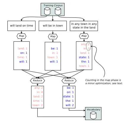
Note that the Reduce function emits only the aggre-gated value. The output key is the same as the inter-mediate key and automatically written by MapRe-duce. The computation of counts in the map func-tion is a minor optimizafunc-tion over the alternative of simply emitting a count of one for each tokenized word in the array. Figure 1 shows an example for 3 input documents and 2 reduce shards. Which re-ducer a particular term is sent to is determined by a hash function, indicated by text color. The exact par-titioning of the keys is irrelevant; important is that all pairs with the same key are sent to the same reducer.

5.2 Generation ofn-Grams

Figure 1: Distributed vocabulary generation.

words. A simplified map function does the follow-ing:

Map(string key, string value) {

// key=docid, ignored; value=document array ids = ToIds(Tokenize(value)); for i = 1 .. #ids

for j = 0 .. maxorder-1 Emit(ids[i-j .. i], "1"); }

Again, one may optimize the Map function by first aggregating counts over some section of the data and then emit the aggregated counts instead of emitting “1” each time ann-gram is encountered.

The reduce function is the same as for vocabu-lary generation. The subsequent step of language model generation will calculate relative frequencies r(wi|w_ii₋−_k1₊₁)(see Eq. 3). In order to make that step

efficient we use a sharding function that places the values needed for the numerator and denominator into the same shard.

Computing a hash function on just the first words of n-grams achieves this goal. The required n-grams wi_i−n+1 and wi_i−−_n1₊₁ always share the same first wordwi−n+1, except for unigrams. For that we

need to communicate the total countNto all shards. Unfortunately, sharding based on the first word only may make the shards very imbalanced. Some terms can be found at the beginning of a huge num-ber of n-grams, e.g. stopwords, some punctuation marks, or the beginning-of-sentence marker. As an example, the shard receiving n-grams starting with

the beginning-of-sentence marker tends to be several times the average size. Making the shards evenly sized is desirable because the total runtime of the process is determined by the largest shard.

The shards are made more balanced by hashing based on the first two words:

int ShardForKey(string key, int nshards) { string prefix = FirstTwoWords(key); return Hash(prefix) % nshards; }

This requires redundantly storing unigram counts in all shards in order to be able to calculate relative fre-quencies within shards. That is a relatively small amount of information (a few million entries, com-pared to up to hundreds of billions ofn-grams).

5.3 Language Model Generation

The input to the language model generation step is the output of the n-gram generation step: n-grams and their counts. All information necessary to calcu-late relative frequencies is available within individ-ual shards because of the sharding function. That is everything we need to generate models with Stupid Backoff. More complex smoothing methods require additional steps (see below).

Backoff operations are needed when the full n-gram is not found. If r(wi|wi_i−−_n1₊₁) is not found,

then we will successively look for r(wi|wii−−1n+2),

r(wi|wi_i−−_n1₊₃), etc. The language model generation

step shards n-grams on their last two words (with unigrams duplicated), so all backoff operations can be done within the same shard (note that the required n-grams all share the same last wordwi).

5.4 Other Smoothing Methods

Step 0 Step 1 Step 2 context counting unsmoothed probs and interpol. weights interpolated probabilities Input key wi

i−n+1 (same as Step 0 output) (same as Step 1 output)

Input value f(wii−n+1) (same as Step 0 output) (same as Step 1 output)

Intermediate key wii−n+1 wii−−1n+1 w

i−n+1

i

Sharding wi

i−n+1 wii−−1n+1 w

i−n+2

i−n+1, unigrams duplicated

Intermediate value fKN(wii−n+1) wi,fKN(wii−n+1)

fK N(wi i₋n+1)−D

fK N(wi−1

i₋n+1)

,λ(wi_i−−1_n+1)

Output value fKN(wii−n+1) wi,

fK N(wii₋n+1)−D

fK N(wi−1

i₋n+1)

,λ(wi−1

i−n+1) PKN(wi|wii−−1n+1),λ(wii−−1n+1)

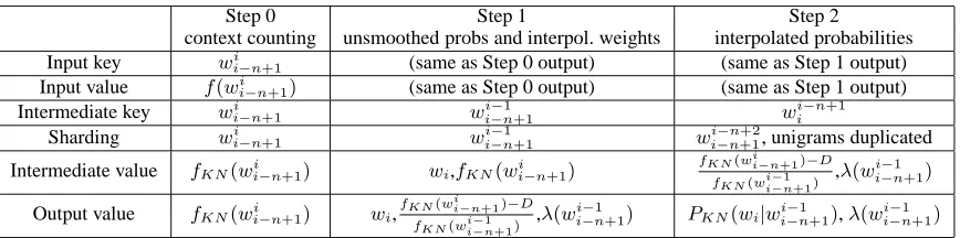
Table 1: Extra steps needed for training Interpolated Kneser-Ney Smoothing

Kneser-Ney Smoothing counts lower-order n-grams differently. Instead of the frequency of the

(n−1)-gram, it uses the number of unique single word contexts the(n−1)-gram appears in. We use fKN(·)to jointly denote original frequencies for the

highest order and context counts for lower orders. After the n-gram counting step, we process the n-grams again to produce these quantities. This can be done similarly to the n-gram counting using a MapReduce (Step 0 in Table 1).

The most commonly used variant of Kneser-Ney smoothing is interpolated Kneser-Ney smoothing, defined recursively as (Chen and Goodman, 1998):

PKN(wi|w_ii₋−_n1₊₁) =

max(fKN(wii−n+1)−D,0)

fKN(wi_i−−_n1₊₁)

+λ(wi_i−−1_n+1)PKN(wi|wii−−1n+2),

whereDis a discount constant and{λ(w_ii₋−1_n+1)}are interpolation weights that ensure probabilities sum to one. Two additional major MapReduces are re-quired to compute these values efficiently. Table 1 describes their input, intermediate and output keys and values. Note that output keys are always the same as intermediate keys.

The map function of MapReduce 1 emitsn-gram histories as intermediate keys, so the reduce func-tion gets all n-grams with the same history at the same time, generating unsmoothed probabilities and interpolation weights. MapReduce 2 computes the interpolation. Its map function emits reversed n-grams as intermediate keys (hence we use wi_i−n+1 in the table). All unigrams are duplicated in ev-ery reduce shard. Because the reducer function re-ceives intermediate keys in sorted order it can com-pute smoothed probabilities for all n-gram orders with simple book-keeping.

Katz Backoff requires similar additional steps. The largest models reported here with Kneser-Ney Smoothing were trained on 31 billion tokens. For Stupid Backoff, we were able to use more than 60 times of that amount.

6 Distributed Application

Our goal is to use distributed language models in-tegrated into the first pass of a decoder. This may yield better results thann-best list or lattice rescor-ing (Ney and Ortmanns, 1999). Dorescor-ing that for lan-guage models that reside in the same machine as the decoder is straight-forward. The decoder accesses n-grams whenever necessary. This is inefficient in a distributed system because network latency causes a constant overhead on the order of milliseconds. On-board memory is around 10,000 times faster.

We therefore implemented a new decoder archi-tecture. The decoder first queues some number of requests, e.g. 1,000 or 10,000 n-grams, and then sends them together to the servers, thereby exploit-ing the fact that network requests with large numbers ofn-grams take roughly the same time to complete as requests with singlen-grams.

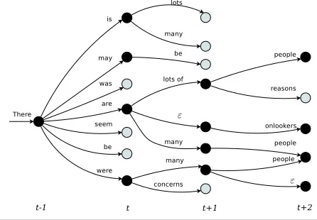
Figure 2: Illustration of decoder graph and batch-querying of the language model.

from other features) decides which hypotheses to keep in the search graph. When using a distributed language model, the decoder first tentatively extends all current hypotheses, taking note of whichn-grams are required to score them. These are queued up for transmission as a batch request. When the scores are returned, the decoder re-visits all of these tentative hypotheses, assigns scores, and re-prunes the search graph. It is then ready for the next round of exten-sions, again involving queuing then-grams, waiting for the servers, and pruning.

The process is illustrated in Figure 2 assuming a trigram model and a decoder policy of pruning to the four most promising hypotheses. The four ac-tive hypotheses (indicated by black disks) at time t are: There is, There may, There are, and There were. The decoder extends these to form eight new nodes at timet+ 1. Note that one of the arcs is labeled , indicating that no target-language word was gener-ated when the source-language word was consumed. Then-grams necessary to score these eight hypothe-ses are There is lots, There is many, There may be, There are lots, are lots of, etc. These are queued up and their language-model scores requested in a batch manner. After scoring, the decoder prunes this set as indicated by the four black disks at timet+ 1, then extends these to form five new nodes (one is shared) at timet+ 2. Then-grams necessary to score these hypotheses are lots of people, lots of reasons, There are onlookers, etc. Again, these are sent to the server together, and again after scoring the graph is pruned to four active (most promising) hypotheses.

The alternating processes of queuing, waiting and scoring/pruning are done once per word position in a source sentence. The average sentence length in our test data is 22 words (see section 7.1), thus we have 23 rounds3per sentence on average. The num-ber of n-grams requested per sentence depends on the decoder settings for beam size, re-ordering win-dow, etc. As an example for larger runs reported in the experiments section, we typically request around 150,000 n-grams per sentence. The average net-work latency per batch is 35 milliseconds, yield-ing a total latency of 0.8 seconds caused by the dis-tributed language model for an average sentence of 22 words. If a slight reduction in translation qual-ity is allowed, then the average network latency per batch can be brought down to 7 milliseconds by re-ducing the number of n-grams requested per sen-tence to around 10,000. As a result, our system can efficiently use the large distributed language model at decoding time. There is no need for a second pass nor forn-best list rescoring.

We focused on machine translation when describ-ing the queued language model access. However, it is general enough that it may also be applicable to speech decoders and optical character recognition systems.

7 Experiments

We trained 5-gram language models on amounts of text varying from 13 million to 2 trillion tokens. The data is divided into four sets; language mod-els are trained for each set separately4. For each training data size, we report the size of the result-ing language model, the fraction of 5-grams from the test data that is present in the language model, and the BLEU score (Papineni et al., 2002) obtained by the machine translation system. For smaller train-ing sizes, we have also computed test-set perplexity using Kneser-Ney Smoothing, and report it for com-parison.

7.1 Data Sets

We compiled four language model training data sets, listed in order of increasing size:

3

One additional round for the sentence end marker. 4

1e+07 1e+08 1e+09 1e+10 1e+11 1e+12

10 100 1000 10000 100000 1e+06 0.1 1 10 100 1000

Number of n-grams

Approx. LM size in GB

LM training data size in million tokens x1.8/x2

x1.8/x2

x1.8/x2

x1.6/x2

target +ldcnews +webnews +web

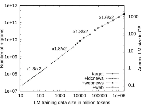
Figure 3: Number ofn-grams (sum of unigrams to 5-grams) for varying amounts of training data.

target: The English side of Arabic-English parallel data provided by LDC5(237 million tokens). ldcnews: This is a concatenation of several English news data sets provided by LDC6(5 billion tokens). webnews: Data collected over several years, up to December 2005, from web pages containing pre-dominantly English news articles (31 billion to-kens).

web: General web data, which was collected in Jan-uary 2006 (2 trillion tokens).

For testing we use the “NIST” part of the 2006 Arabic-English NIST MT evaluation set, which is not included in the training data listed above7. It consists of 1797 sentences of newswire, broadcast news and newsgroup texts with 4 reference tions each. The test set is used to calculate transla-tion BLEU scores. The English side of the set is also used to calculate perplexities andn-gram coverage.

7.2 Size of the Language Models

We measure the size of language models in total number of n-grams, summed over all orders from 1 to 5. There is no frequency cutoff on then-grams.

5_{http://www.nist.gov/speech/tests/mt/doc/}

LDCLicense-mt06.pdfcontains a list of parallel resources provided by LDC.

6

The bigger sets included are LDC2005T12 (Gigaword, 2.5B tokens), LDC93T3A (Tipster, 500M tokens) and LDC2002T31 (Acquaint, 400M tokens), plus many smaller sets.

7

The test data was generated after 1-Feb-2006; all training data was generated before that date.

target webnews web # tokens 237M 31G 1.8T vocab size 200k 5M 16M

#n-grams 257M 21G 300G

LM size (SB) 2G 89G 1.8T time (SB) 20 min 8 hours 1 day time (KN) 2.5 hours 2 days – # machines 100 400 1500

Table 2: Sizes and approximate training times for 3 language models with Stupid Backoff (SB) and Kneser-Ney Smoothing (KN).

There is, however, a frequency cutoff on the vocab-ulary. The minimum frequency for a term to be in-cluded in the vocabulary is 2 for the target, ldcnews and webnews data sets, and 200 for the web data set. All terms below the threshold are mapped to a spe-cial termUNK, representing the unknown word.

Figure 3 shows the number of n-grams for lan-guage models trained on 13 million to 2 trillion to-kens. Both axes are on a logarithmic scale. The right scale shows the approximate size of the served language models in gigabytes. The numbers above the lines indicate the relative increase in language model size: x1.8/x2 means that the number of n-grams grows by a factor of 1.8 each time we double the amount of training data. The values are simi-lar across all data sets and data sizes, ranging from 1.6 to 1.8. The plots are very close to straight lines in the log/log space; linear least-squares regression findsr2>0.99for all four data sets.

The web data set has the smallest relative increase. This can be at least partially explained by the higher vocabulary cutoff. The largest language model gen-erated contains approx. 300 billionn-grams.

50 100 150 200 250 300 350

10 100 1000 10000 100000 1e+06 0 0.1 0.2 0.3 0.4 0.5 0.6

Perplexity

Fraction of covered 5-grams

LM training data size in million tokens +.022/x2

+.035/x2

+.038/x2 +.026/x2

target KN PP ldcnews KN PP webnews KN PP target C5 +ldcnews C5 +webnews C5 +web C5

Figure 4: Perplexities with Kneser-Ney Smoothing (KN PP) and fraction of covered 5-grams (C5).

7.3 Perplexity andn-Gram Coverage

A standard measure for language model quality is perplexity. It is measured on test dataT =w|₁T|:

P P(T) =e−

1 |T|

|T|

i=1

logp(wi|wii−−1n+1)

(7)

This is the inverse of the average conditional prob-ability of a next word; lower perplexities are bet-ter. Figure 4 shows perplexities for models with Kneser-Ney smoothing. Values range from 280.96 for 13 million to 222.98 for 237 million tokens tar-get data and drop nearly linearly with data size (r2= 0.998). Perplexities for ldcnews range from 351.97 to 210.93 and are also close to linear (r2 = 0.987), while those for webnews data range from 221.85 to 164.15 and flatten out near the end. Perplexities are generally high and may be explained by the mix-ture of genres in the test data (newswire, broadcast news, newsgroups) while our training data is pre-dominantly written news articles. Other held-out sets consisting predominantly of newswire texts re-ceive lower perplexities by the same language mod-els, e.g., using the full ldcnews model we find per-plexities of 143.91 for the NIST MT 2005 evaluation set, and 149.95 for the NIST MT 2004 set.

Note that the perplexities of the different language models are not directly comparable because they use different vocabularies. We used a fixed frequency cutoff, which leads to larger vocabularies as the training data grows. Perplexities tend to be higher with larger vocabularies.

0.34 0.36 0.38 0.4 0.42 0.44

10 100 1000 10000 100000 1e+06

Test data BLEU

LM training data size in million tokens +0.62BP/x2

+0.56BP/x2

+0.51BP/x2

+0.66BP/x2

+0.70BP/x2

+0.39BP/x2

+0.15BP/x2

target KN +ldcnews KN +webnews KN target SB +ldcnews SB +webnews SB +web SB

Figure 5: BLEU scores for varying amounts of data using Kneser-Ney (KN) and Stupid Backoff (SB).

Perplexities cannot be calculated for language models with Stupid Backoff because their scores are not normalized probabilities. In order to neverthe-less get an indication of potential quality improve-ments with increased training sizes we looked at the gram coverage instead. This is the fraction of 5-grams in the test data set that can be found in the language model training data. A higher coverage will result in a better language model if (as we hy-pothesize) estimates for seen events tend to be bet-ter than estimates for unseen events. This fraction grows from 0.06 for 13 million tokens to 0.56 for 2 trillion tokens, meaning 56% of all 5-grams in the test data are known to the language model.

Increase in coverage depends on the training data set. Within each set, we observe an almost constant growth (correlation r2 ≥ 0.989 for all sets) with each doubling of the training data as indicated by numbers next to the lines. The fastest growth oc-curs for webnews data (+0.038 for each doubling), the slowest growth for target data (+0.022/x2).

7.4 Machine Translation Results

We use a state-of-the-art machine translation system for translating from Arabic to English that achieved a competitive BLEU score of 0.4535 on the Arabic-English NIST subset in the 2006 NIST machine translation evaluation8. Beam size and re-ordering window were reduced in order to facilitate a large

8

number of experiments. Additionally, our NIST evaluation system used a mixture of 5, 6, and 7-gram models with optimized stupid backoff factors for each order, while the learning curve presented here uses a fixed order of 5 and a single fixed backoff fac-tor. Together, these modifications reduce the BLEU score by 1.49 BLEU points (BP)9at the largest train-ing size. We then varied the amount of language model training data from 13 million to 2 trillion to-kens. All other parts of the system are kept the same. Results are shown in Figure 5. The first part of the curve uses target data for training the lan-guage model. With Kneser-Ney smoothing (KN), the BLEU score improves from 0.3559 for 13 mil-lion tokens to 0.3832 for 237 milmil-lion tokens. At such data sizes, Stupid Backoff (SB) with a constant backoff parameter α = 0.4 is around 1 BP worse than KN. On average, one gains 0.62 BP for each doubling of the training data with KN, and 0.66 BP per doubling with SB. Differences of more than 0.51 BP are statistically significant at the0.05level using bootstrap resampling (Noreen, 1989; Koehn, 2004). We then add a second language model using ldc-news data. The first point for ldcldc-news shows a large improvement of around 1.4 BP over the last point for target for both KN and SB, which is approxi-mately twice the improvement expected from dou-bling the amount of data. This seems to be caused by adding a new domain and combining two models. After that, we find an improvement of 0.56–0.70 BP for each doubling of the ldcnews data. The gap be-tween Kneser-Ney Smoothing and Stupid Backoff narrows, starting with a difference of 0.85 BP and ending with a not significant difference of 0.24 BP.

Adding a third language models based on web-news data does not show a jump at the start of the curve. We see, however, steady increases of 0.39– 0.51 BP per doubling. The gap between Kneser-Ney and Stupid Backoff is gone, all results with Stupid Backoff are actually better than Kneser-Ney, but the differences are not significant.

We then add a fourth language model based on web data and Stupid Backoff. Generating Kneser-Ney models for these data sizes is extremely ex-pensive and is therefore omitted. The fourth model

9

1 BP = 0.01 BLEU. We show system scores as BLEU, dif-ferences as BP.

shows a small but steady increase of 0.15 BP per doubling, surpassing the best Kneser-Ney model (trained on less data) by 0.82 BP at the largest size. Goodman (2001) observed that Kneser-Ney Smoothing dominates other schemes over a broad range of conditions. Our experiments confirm this advantage at smaller language model sizes, but show the advantage disappears at larger data sizes.

The amount of benefit from doubling the training size is partly determined by the domains of the data sets10. The improvements are almost linear on the log scale within the sets. Linear least-squares regres-sion shows correlations r2 > 0.96 for all sets and both smoothing methods, thus we expect to see sim-ilar improvements when further increasing the sizes.

8 Conclusion

A distributed infrastructure has been described to train and apply large-scale language models to ma-chine translation. Experimental results were pre-sented showing the effect of increasing the amount of training data to up to 2 trillion tokens, resulting in a 5-gram language model size of up to 300 billion n-grams. This represents a gain of about two orders of magnitude in the amount of training data that can be handled over that reported previously in the liter-ature (or three-to-four orders of magnitude, if one considers only single-pass decoding). The infra-structure is capable of scaling to larger amounts of training data and highern-gram orders.

The technique is made efficient by judicious batching of score requests by the decoder in a server-client architecture. A new, simple smoothing tech-nique well-suited to distributed computation was proposed, and shown to perform as well as more sophisticated methods as the size of the language model increases.

Significantly, we found that translation quality as indicated by BLEU score continues to improve with increasing language model size, at even the largest sizes considered. This finding underscores the value of being able to train and apply very large language models, and suggests that further performance gains may be had by pursuing this direction further.

10

References

Peter F. Brown, Stephen Della Pietra, Vincent J. Della Pietra, and Robert L. Mercer. 1993. The mathematics of statistical machine translation: Parameter estima-tion. Computational Linguistics, 19(2):263–311.

Stanley F. Chen and Joshua Goodman. 1998. An empiri-cal study of smoothing techniques for language model-ing. Technical Report TR-10-98, Harvard, Cambridge, MA, USA.

Jeffrey Dean and Sanjay Ghemawat. 2004. Mapreduce: Simplified data processing on large clusters. In Sixth

Symposium on Operating System Design and Imple-mentation (OSDI-04), San Francisco, CA, USA.

Ahmad Emami, Kishore Papineni, and Jeffrey Sorensen. 2007. Large-scale distributed language modeling. In

Proceedings of ICASSP-2007, Honolulu, HI, USA.

Joshua Goodman. 2001. A bit of progress in language modeling. Technical Report MSR-TR-2001-72, Mi-crosoft Research, Redmond, WA, USA.

Frederick Jelinek and Robert L. Mercer. 1980. Inter-polated estimation of Markov source parameters from sparse data. In Pattern Recognition in Practice, pages 381–397. North Holland.

Slava Katz. 1987. Estimation of probabilities from sparse data for the language model component of a speech recognizer. IEEE Transactions on Acoustics,

Speech, and Signal Processing, 35(3).

Reinhard Kneser and Hermann Ney. 1995. Improved backing-off for m-gram language modeling. In

Pro-ceedings of the IEEE International Conference on Acoustics, Speech and Signal Processing, pages 181–

184.

Philipp Koehn. 2004. Statistical significance tests for machine translation evaluation. In Proceedings of

EMNLP-04, Barcelona, Spain.

Hermann Ney and Stefan Ortmanns. 1999. Dynamic programming search for continuous speech recogni-tion. IEEE Signal Processing Magazine, 16(5):64–83.

Eric W. Noreen. 1989. Computer-Intensive Methods for

Testing Hypotheses. John Wiley & Sons.

Franz Josef Och and Hermann Ney. 2004. The align-ment template approach to statistical machine transla-tion. Computational Linguistics, 30(4):417–449.

Kishore Papineni, Salim Roukos, Todd Ward, and Wei-Jing Zhu. 2002. BLEU: a method for automatic eval-uation of machine translation. In Proceedings of

ACL-02, pages 311–318, Philadelphia, PA, USA.