Part-of-Speech Tagging using Virtual Evidence and Negative Training
Sheila M. Reynolds and Jeff A. Bilmes
Department of Electrical Engineering University of Washington
Seattle, WA 98195-2500
{sheila,bilmes}@ee.washington.edu
Abstract
We present a part-of-speech tagger which introduces two new concepts: virtual evi-dence in the form of an “observed child” node, and negative training data to learn the conditional probabilities for the ob-served child. Associated with each word is a flexible feature-set which can in-clude binary flags, neighboring words, etc. The conditional probability of Tag given
Word + Features is implemented using a factored language-model with back-off to avoid data sparsity problems. This model remains within the framework of Dynamic Bayesian Networks (DBNs) and is conditionally-structured, but resolves the label bias problem inherent in the con-ditional Markov model (CMM).
1 Introduction
A common sequence-labeling task in natural lan-guage processing involves assigning a part-of-speech (POS) tag to each word in the input text. Previous authors have used numerous HMM-based models (Banko and Moore, 2004; Collins, 2002; Lee et al., 2000; Thede and Harper, 1999) and other types of networks including maximum entropy models (Ratnaparkhi, 1996), conditional Markov models (Klein and Manning, 2002; McCallum et al., 2000), conditional random fields (CRF) (Laf-ferty et al., 2001), and cyclic dependency networks (Toutanova et al., 2003). All of these models make
use of varying amounts of contextual information. In this paper, we present a new model which re-mains within the well understood framework of Dy-namic Bayesian Networks (DBNs), and we show that it produces state-of-the-art results when ap-plied to the POS-tagging task. This new model is conditionally-structured and, through the use of vir-tual evidence (Pearl, 1988; Bilmes, 2004), resolves the explaining-away problems (often described as label or observation bias) inherent in the CMM.
This paper is organized as follows. In sec-tion 2 we discuss the differences between a hidden Markov model (HMM) and the corresponding con-ditional Markov model (CMM). In section 3 we de-scribe our observed-child model (OCM), introduc-ing the notion of virtual evidence, and providintroduc-ing an information-theoretic foundation for the use of nega-tive training data. In section 4 we discuss our exper-iments and results, including a comparison of three simple first-order models and state-of-the-art results from our feature-rich second-order OCM.
For clarity, the comparisons and derivations in sections 2 and 3 are done for first-order models us-ing a sus-ingle binary feature. The same ideas are then generalized to a higher order model with more fea-tures (including adjacent words).
2 Generative vs. Conditional Models In this section we discuss the tradeoffs between the generative hidden Markov model (HMM) and the conditional Markov model (CMM). For pedagogical reasons, the figures and equations are for first order models with a single word-feature.
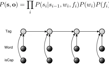
The HMM shown in Figure 1 includes a single
feature (the binary flag isCap) in addition to the word itself. Each observation, oi = (wi, fi), is a
word-feature pair. Leto = {oi}be the observation
sequence ands ={si}be the associated tag (state)
sequence. The HMM1factorizes the joint probabil-ity distribution over these two sequences as:
P(s,o) =Y
i
P(si|si−1)P(wi|si)P(fi|si)
Tag
Word
[image:2.612.95.278.149.263.2]isCap
Figure 1: First order HMM.
A similar model often used for sequence label-ing tasks is the conditional Markov model (CMM) which reverses the arrows between the words and the tags (Figure 2), and factorizes as:
P(s,o) =Y
i
P(si|si−1, wi, fi)P(wi)P(fi)
Tag
Word
isCap
Figure 2: First order CMM.
Because the words and features are observed, this model does not require that we compute the proba-bility of the evidence, P(o), when finding the
opti-mal tag sequence. The tag-sequence s which
max-imizes the joint probabilityP(s,o)is the same one
that maximizes the conditionalprobability P(s|o).
The CMM, therefore, does not require that we model the language, allowing us to focus on modeling the conditional probability of the tags given the words.
The HMM has its advantages as well, principally that it is easier to train than the CMM because it 1In this HMM, Word and isCap are independent given Tag,
but this need not be true in general.
factorizes the joint probability into simpler com-ponents. The tables required for P(si|si−1) and P(oi|si) are significantly smaller than the one for P(si|si−1, oi)which may be difficult to estimate due
to either data sparsity or normalization issues. One potential disadvantage of the HMM is that when it is trained using a maximum likelihood procedure, it is not necessarily encouraged to optimally classify tags due to its generative nature. One solution is to train the HMM using a discriminative procedure. Another option is to use entirely different models.
A key disadvantage of the CMM is that it makes critical statements about independence that the HMM does not: the converging arrows at each tag put the parent nodes (the previous tag and the current observation) into causal competition and as a result the model states that the previous tag is inde-pendent of the current observation. In other words, all states (tags) are independent of future observa-tions (words). The CMM thus incorporates a strong directional bias which does not exist in the HMM.
One way to eliminate this bias is to use a CRF (Lafferty et al., 2001; McCallum, 2003), where fac-tors over neighboring tags may use features from anywhere in the observation sequence. The CRF is discriminative and avoids label/observation bias by using a model that is constrained only in that the conditional distribution factorizes over an undi-rected Markov chain. However, most popular train-ing procedures for a CRF are time-consumtrain-ing and complex processes.
3 Using Virtual Evidence
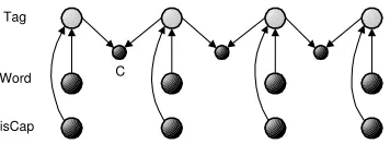
Our goals in this work are to: 1) keep the discrimi-native nature of the CMM to the extent possible; 2) avoid label and observation bias issues; and 3) stay entirely within the DBN framework where training is relatively simple. We thus propose a new solu-tion to the problem, which retains the discrimina-tive conditional form of “tag given word” from the CMM, but avoids label bias by temporally linking adjacent tags in a new way. Specifically, we employ virtual evidence in the form of a binary observed child node, ci, between adjacent tags (Figure 3) or
[image:2.612.90.280.372.492.2]Tag
Word
isCap
[image:3.612.98.276.53.119.2]C
Figure 3: First order observed-child model (OCM) with the tags connected in pairs.
tag-pair consistency. When the tag pairs are consis-tent (as they are in real text), we should have a high conditional probability that ci = 1; and when the
tag pairs are not consistent, the conditional probabil-ity thatci = 1should be low. With this conditional
distribution, observing ci = 1during decoding
ex-presses a preference for consistent tag pairs.
The presence of this observed-child node results in a term in the factorization of the joint probability distribution that couples its parents:
P(c,s,o) ∝Y
i
P(ci|si−1, si)P(si|wi, fi)
whereciis the observed-child node of tagssi−1and si, and we omit the probability of the observations, P(wi, fi)which do not affect the final choice ofs.
By the rules of d-separation (Pearl, 1988), the ex-istence ofci defined in this way means that the
par-ents (the adjacent tags) are not conditionally inde-pendent given the child. This link between adja-cent tags through an observed-child node allows for a probabilistic relationship to exist between the ad-jacent tags. Thus, future words can influence tags, which is not true for the CMM. Whether or not a relationship between tags will actually be learned, however, will critically depend on how the model is trained. In a graphical model, it is the lack of an edge that ensures some form of independence; the presence of an edge (or a path made up of two or more edges) does not necessarily ensure the reverse.
3.1 Training
The introduction of virtual evidence into a graph-ical model requires that careful thought be given to the training process. If we were to na¨ıvely add
ci = 1to all samples of the training data, the model
would learn that ci is constant rather than random,
and therefore that it is independent of its parents,
si−1 and si. In other words, this na¨ıvely-trained
model would assume that P(ci = 1|si−1, si) =
1 ∀ (si−1, si), and when used to tag the sentences
in the test-set (also labeled with ci = 1), it would
maximize this simplified joint probability in which the relationship betweensi−1andsi has been lost:
P(c,s,o)∝Y
i
P(si|wi, fi)
In order to induce and thereby have the model
learnthe relationship between the adjacent tagssi−1
and si, the training has to be modified to include
samples that are labeled withci = 0. The
proba-bility tableP(ci= 1|si−1, si)should favor common
(consistent) tag-pairs with high probabilities, while discouraging rare tag-pairs with low probabilities.
Although all observations (in both training and test sets) are labeled with ci = 1, we hypothesize
an alternate set of observations labeled withci = 0.
This alternate set will be the source of the negative training data 2. It is a set of nonsensical sentences with the same distribution over individual tags, i.e. the sameP(si), but in this set adjacent tags are
in-dependent. We denote the total number of training samples by M. This is divided into positive
train-ing samples,M1, and negative training samples,M0,
withM1+M0 =M. The ratio of the amount of
pos-itive to negative training data should be the same as the ratio of our prior beliefs about tag-pair consis-tency, namely the ratio ofP(ci = 1)toP(ci = 0).
With no evidence to support that one is more likely than the other, one option is to use the strategy of “assuming the least” and use a maximum entropy prior, settingM0 = M1. More flexibly, we can de-finento be the ratio of the two so thatM0 =n·M1. Now we derive a method for training the condi-tional probability tableP(ci|si−1, si)in terms of the
pointwise mutual information between the adjacent tags si−1 and si. We first rewrite the conditional
probability (henceforth abbreviated asp) as:
p=P(ci= 1|si−1, si) =
P(ci= 1, si−1, si) P(si−1, si)
If the probabilities are maximum likelihood (ML) estimates derived from counts on the training data, we can equivalently write:
p= N(ci = 1, si−1, si)
N(si
−1, si)
2This use of implied negative training data is similar to the
whereN(·) is the count function.
Expanding the denominator into two terms:
p= N(ci = 1, si−1, si)
N(ci = 1, si
−1, si) +N(ci = 0, si−1, si)
Without any negative training data (labeled with
ci = 0), this ratio would always evaluate to 1, and no
probabilistic relationship betweensi−1andsiwould
be learned.
From the start, we have implicitly postulated a re-lationship between adjacent tags. We now formally state two hypotheses: H1that thereisa relationship between adjacent tags which can be described by some joint probability distribution P(si−1, si), and
the null hypothesis, H0, that there is no such rela-tionship, i.e.si−1andsi are independent:
PH1 =P(si−1, si)
PH0 =P(si−1)P(si)
Now we can express the counts as follows:
N(ci= 1, si
−1, si) =M1·P(si−1, si)
N(ci= 0, si
−1, si) =M0·P(si−1)P(si)
whereM1is the total number of tokens in the (posi-tive) training data, andM0is the total number of to-kens in the induced negative training data. We sub-stitute M0 with n ·M1 for the reasons mentioned earlier, and simplify to obtain:
p= P(si−1, si)
P(si−1, si) +nP(si−1)P(si)
which can be simplified to obtain:
p= 1
1 +n
P(si −1,si)
P(si−1)P(si) −1
The ratio of probabilities in the denominator is the ratio used in computing the pointwise mutual infor-mation between si−1 and si. This ratio, which we
will call λ, is also the likelihood ratio between the
two previously stated hypotheses. Finally, we write the conditional probability as a function ofλ:
P(ci = 1|si−1, si) =
1 1 +nλ−1 =
λ λ+n
where λ= PH1
PH0
= P(si−1, si) P(si−1)P(si)
= P(si|si−1) P(si)
The conditional probability, P(ci = 1|si−1, si)is a
mappingg(λ)fromλ∈[0,∞)top∈[0,1). Beginning with (Church and Hanks, 1989), nu-merous authors have used the pointwise mutual in-formation between pairs of words to analyze word co-locations and associations. This ratio tells us whethersi−1andsico-occur more or less often than
would be expected by chance alone.
Consider, for example, the tags DT (determiner) and NN (noun), and the four possible ordered tag-pairs. The probabilities P(si) and P(si|si−1)
de-rived from the training data (see section 4.1), the likelihood ratio scoreλ, the conditional probability p = P(ci = 1|si−1, si), and the occurrence counts Nare shown in Table 1. As expected, the sequence DT-NN (e.g.the surplus) occurs very often and gets a high score, while DT-DT (e.g. this a) and NN-DT (e.g.surplus the) occur infrequently and get low scores. The sequence NN-NN (e.g. trade surplus) gets a neutral score (λ≈1) indicating that if the pre-ceding word is a noun, the likelihood that the current word is a noun is nearly equal to the likelihood that any randomly chosen word is a noun.
We present two methods for inducing the negative training counts that are required to train the condi-tional probability table forP(ci|si−1, si).
In the first method, we generate “nonsense” sen-tences by randomly scrambling each sentence in the training-set n times, using a uniform distribution
over all possible permutations. This results in n
negative training sentences for each positive training sentence and thereforeM0=n·M1. Effectively, the ratio of priors onci is now:
P(ci = 1) P(ci = 0)
= M1
M0 = 1
n
The conditional probability table P(ci|si−1, si) is
si
−1-si P(si) P(si|si−1) λ p N
DT-NN 0.129 0.4905 3.80 0.79 37301
NN-NN 0.129 0.1270 0.98 0.49 15571
NN-DT 0.080 0.0071 0.09 0.08 870
DT-DT 0.080 0.0018 0.02 0.02 134
Table 1: Sample likelihood ratio scores (λ),
then trained using alln+1versions of each sentence, thus inducing the desired dependence betweensi−1
andsi. The method of scrambling sentencesn-times
only approximates the theory described above be-cause it is performed on a sentence-by-sentence ba-sis rather than across the entire training set. Also, the resulting negative training data represents onlyn
re-alizations of a random process, so the total number of samples may not be large enough to approximate the underlying distribution.
In the second method, rather than generate the negative training data in the form of scrambled sen-tences, we compute the negative-training counts di-rectly, based on the positive unigram counts and the hypotheses presented in section 3.1. For example, the negative bigram counts are a function of the marginal probability of each tag,P(si):
N(ci= 0, si
−1, si) =nM1·P(si−1)P(si)
Negative unigram and trigram counts are computed in a similar fashion, and then the conditional proba-bility table is derived as a smoothed back-off model directly from the combined sets of counts.
These two methods are conceptually similar but may exhibit subtle differences: one is randomizing at the sentence level while the other operates over the entire training set and does not have the same sensitivity to small values ofn.
4 Experiments and Results
In this section we describe our experiments and the results obtained. Sections 4.1 and 4.2 describe the data sets and features. Section 4.3 presents compar-isons between several simple models using just the tags, the words, and a single binary feature for each word. Section 4.4 presents results from a feature-rich second-order observed-child model in which tags are linked in groups of three.
All training of language models is done using the SRILM toolkit (Stolcke, 2002) with the FLM exten-sions (Bilmes and Kirchhoff, 2003), and the imple-mentation and testing of the various graphical els is carried out with the help of the graphical mod-els toolkit (GMTK) (Bilmes and Zweig, 2002).
4.1 Data Sets
The data used for these experiments is the Wall Street Journal data from Penn Treebank III
(Mar-cus et al., 1994). We extracted tagged sentences from the parse trees and divided the data into train-ing (sections 0-18), development (sections 19-21), and test (sections 22-24) sets as in (Toutanova et al., 2003). Except for the final results for the feature-rich model, all results are on the development set.
4.2 Features
The tagged sentences extracted from the Penn Tree-bank are pre-processed to generate appropriately-formatted training data for the SRILM toolkit, as well as the vocabulary and observation files to be used during testing.
The pre-processing includes building a dictionary based on the training data. All words containing uppercase letters are converted to lowercase before being written to the dictionary. Words that occur rarely are excluded from the dictionary and are in-stead mapped to a single out-of-vocabulary word. This is based on the idea from (Ratnaparkhi, 1996) that rare words in the training set are similar to un-known words in the test set, and can be used to learn how to tag the unknown words that will be encoun-tered during testing. In this work, rare words are those that occurr fewer than 5 times. The dictio-nary also includes special begin-sentence and end-sentence words, as well as punctuation marks, re-sulting in a total of 10,824 words. A list of the 45 tags found in the training data is also created, and is similarly augmented with special begin-sentence
andend-sentence tags, for a total of 47 distinct tags. Each word has associated with it a set of features. During training, these features are used to learn a smoothed back-off model forP(si|wi,fi)(wherefi
is a vector of features associated with wordwi).
The following five binary flags, taken from (Toutanova et al., 2003), are derived from the cur-rent wordwiand used as features :
• is-capitalized (refers to the first letter only); • has-digits (word contains one or more digits); • is-hyphenated (word contains ‘-’);
• is-all-caps (allletters are capitalized);
• is-conjunction (true if is-all-caps, has-digits,
and is-hyphenated are all true, for example
CFC-12orF/A-18).
suffix-feature to our set. Previous work used all possible prefixes and suffixes ranging in length from 1 to k
characters, with k = 4 (Ratnaparkhi, 1996), and
k = 10 (Toutanova et al., 2003). This method re-sults in very long lists of thousands of suffixes and prefixes. In this work, we instead analyzed the rare words in the training data to generate shorter lists of informative prefixes and suffixes, with lengths be-tween 1 and 7 characters. Each prefix/suffix was scored based on the number of times it appeared with a particular tag, and all prefixes/suffixes that scored above 20 (an arbitrarily chosen threshold) were kept. This process resulted in two separate lists: one with 377 prefixes, and the other with 704 suffixes. Each word is then assigned a single pre-fix feature and a single sufpre-fix feature from these lists (which both include an entry for “unknown”). When assigning prefix and suffix features to the rare words (in the training data) or the unknown words (in the test data), we assume that the longest string is the most informative. (This may not necessarily be true: for example, although the suffixingis certainly more informative thang, it is less clear whether ulat-ingwould be more or less informative thaning.)
We also include the two adjacent words as fea-tures of the current word. Our model provides great flexibility in the choice of features to be included in the current word’s feature-set. This feature-set is not limited to binary flags and indeed can include anything that can be extracted from the observa-tion sequence in the pre-processing stage. By using a smoothed back-off model, issues related to data-sparsity and over-fitting are avoided.
4.3 First Order Model Comparisons
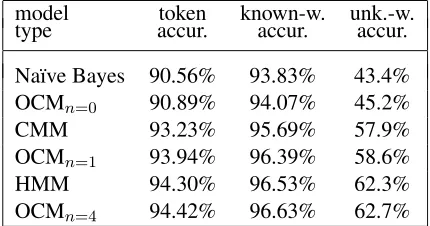
In this section we compare results obtained from three first-order models: HMM, CMM, and OCM, using a Na¨ıve Bayes (NB) model as a baseline. The Na¨ıve Bayes model is a zeroth-order model with no connection between adjacent tags, while the first-order models connect adjacent tags in pairs. (Note that the HMM in this case is just a “temporal” NB since given the tag, the features are independent.) In these experiments, the only feature used is the is-capitalized flag (the most informative of the binary flags tested). The results are shown in Table 2.
The conditional probability tables (CPTs) for the CMM and the OCM were generated using the
model token known-w. unk.-w.
type accur. accur. accur.
Na¨ıve Bayes 90.56% 93.83% 43.4% OCMn=0 90.89% 94.07% 45.2%
CMM 93.23% 95.69% 57.9%
OCMn=1 93.94% 96.39% 58.6%
HMM 94.30% 96.53% 62.3%
[image:6.612.319.534.56.169.2]OCMn=4 94.42% 96.63% 62.7%
Table 2: Scores for first order models.
factored language model (FLM) extensions to the SRILM toolkit, wth generalized parallel backoff and Witten-Bell smoothing. (Modified Kneser-Ney smoothing could not be applied because some of the required low-order meta-counts needed by the dis-count estimator were zero.) The negative training data for the OCM was generated using the scram-ble method, with values ofnas in the table. When
no negative training data is used (n = 0), the CPT for the observed-child shows a very weak depen-dence on the specific tag-pair(si−1, si): the
proba-bility values in the tag-bigram model range only be-tween0.89and1. This weak dependence results in performance comparable to that of the Na¨ıve Bayes model. That there is any dependence at all is due to the smoothing sinceci = 0is never observed in the
training data. With negative training data (n = 4), there is a much stronger dependence on the tag-pair, and the values forP(ci = 1|si−1, si)range between
0.0002and1.
We found experimentally that the OCM reached peak performance withn = 4and that for largern
the performance stayed relatively constant: the vari-ation for values ofnup to14was only0.05%.
4.4 Feature-Rich Second-Order OCM
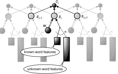
In this section we describe the results obtained from a more complex second order OCM with the addi-tional word features described in section 4.2.
This model is illustrated in Figure 4 which, for clarity highlights the details only for one (tag,word) pair. The observed-child node,ci, now has three
par-ents: the tags si−1, si, and si+1. Each tag, si, in
turn has K + 1parents: the current word, wi, and
a set of K features (shown bundled together). The
model description token known-word unknown-word accuracy accuracy accuracy
OCM-I, scramble,n= 4 96.39% 96.87% 89.5%
[image:7.612.129.485.56.157.2]OCM-I, computed counts,n= 4 96.41% 96.90% 89.3% OCM-I, computed counts,n= 1 96.41% 96.92% 89.0% OCM-II, computed counts,n= 1 96.64% 97.12% 89.5% OCM-II, as above, on test-set 96.77% 97.25% 90.0%
Table 3: Tagging accuracy using the feature-rich 2ndorder observed-child model.
illustrated, based on the current word. For known words, a small set of features is used, while a much larger set of features is used for unknown words. This switching increases the speed of the model at no cost: the additional features increase the tagging accuracy for unknown words but are redundant for known words.
This model factorizes the joint probability as:
P(c,s,o)∝Y
i
P(ci|si−1, si, si+1)P(si|wi,fi)
wherefi is the appropriate feature bundle for word
wi, depending on whetherwiis known or unknown.
ci
si-1 si si+1
wi
known-word features
unknown-word features
Figure 4: Second order OCM with tags connected in triples and switching sets of word features.
Two sets of experiments were performed using two models, which we will refer to as OCM-I and OCM-II. Both of these are second order models (connecting tags in triples), but with different sets of features. In model OCM-I, the only feature used for known words is the is-capitalized flag used in section 4.3. The unknown words use a total of seven features: suffix, prefix, and all five of the binary flags described in section 4.2. Model OCM-II adds the
ad-jacent words (wi−1 and wi+1) to the feature-set for
both known and unknown words.
As seen above, the model factorizes the joint probability into two conditional probability terms. Each of these CPTs is implemented as a smoothed, factored-language back-off model.
The observed-child CPT uses generalized back-off, combining at run-time the results of backing off from each of the three parents if the specific tag-triple is not found in the table. The tag CPT uses linear backoff, dropping the adjacent words first. The backoff order for the other features was cho-sen based on experiments to determine the relative information content of each feature. This resulted in the following backoff order: prefix, has-digit, conjunction, all-caps, hyphenated, suffix, is-capitalized, word (where the least informative fea-ture, prefix, is the first feature to be dropped).
Results from these experiments are shown in Ta-ble 3. Except for the last line, which reports results on the test set, all results are on the development set. The first three lines show results obtained from OCM-I (without adjacent word features). The two methods of generating negative training data yield nearly identical results, showing that they are com-parable. Comparing rows 2 and 3 in the table we see that the computed-counts method is relatively insen-sitive to the value ofn(forn≥1).
[image:7.612.89.287.403.527.2]5 Conclusions
In this paper, we have introduced two new concepts to the problem of part-of-speech tagging: virtual evi-dence and negative training data. We have moreover shown that this new model can produce state-of-the-art results on this NLP task with appropriately cho-sen features. The model stays entirely within the mathematically formal language of Bayesian net-works, and even though it is conditional in nature, the model does not suffer from label or observa-tion (or direcobserva-tional) bias. Staying within this frame-work has other advantages as well, including that the training procedures remain within the relatively simple maximum likelihood framework, albeit with appropriate smoothing. We believe that this model holds great promise for other NLP tasks as well as in other applications of machine-learning such as com-putational biology. In particular the way it factor-izes the joint probability into a “horizontal” com-ponent which connects various nodes to the virtual-evidence node, and a “vertical” component (used here to link a tag to a set of observations), provides great simplicity, flexibility, and power.
6 Acknowledgements
The authors would like to thank the anonymous re-viewers for their constructive comments. Sheila Reynolds is supported by an NDSEG fellowship.
References
Michele Banko and Robert C. Moore. 2004. Part of Speech Tagging in Context.Proceedings of COLING.
Jeff Bilmes. 2004. On Soft Evidence in Bayesian Net-works. Tech. Rep. UWEETR-2004-0016, U. Wash-ington Dept. of Electrical Engineering, 2004.
Jeff Bilmes and Katrin Kirchhoff. 2003. Factored lan-guage models and generalized parallel backoff. Pro-ceedings of HLT-NAACL: Short Papers, 4-6.
Jeff Bilmes and Geoffrey Zweig. 2002. The graphi-cal models toolkit: An open source software system for speech and time-series processing. Proceedings of ICASSP, vol4, 3916-3919.
Kenneth W. Church and Patrick Hanks. 1989. Word As-sociation Norms, Mutual Information, and Lexicogra-phy.Proceedings of ACL, 76-83.
Michael Collins. 2002. Discriminative Training Meth-ods for Hidden Markov Models: Theory and Experi-ments with Perceptron Algorithms.Proc. EMNLP.
Dan Klein and Christopher D. Manning. 2002. Condi-tional Structure versus CondiCondi-tional Estimation in NLP Models.Proceedings of EMNLP, 9-16.
John Lafferty, Andrew McCallum and Fernando Pereira. 2001. Conditional Random Fields: Probabilistic Mod-els for Segmenting and Labeling Sequence Data. Pro-ceedings of ICML, 282-289.
Sang-Zoo Lee, Jun-ichi Tsujii and Hae-Chang Rim. 2000. Part-of-Speech Tagging Based on Hidden Markov Model Assuming Joint Independence. Pro-ceedings of 38th ACL, 263-269.
Mitchell P. Marcus, Beatrice Santorini and Mary A. Marcinkiewicz. 1994. Building a large annotated cor-pus of English: The Penn Treebank. Computational Linguistics, 19:313-330.
Andrew McCallum. 2003. Efficiently Inducing Features of Conditional Random Fields.Proceedings of UAI.
Andrew McCallum, Dayne Freitag and Fernando Pereira. 2000. Maximum-Entropy Markov Models for Infor-mation Extraction and Segmentation. Proc. 17th In-ternational Conf. on Machine Learning, 591-598. Judea Pearl. 1988. Probabilistic Reasoning in
Intelli-gent Systems: Networks of Plausible Inference. Mor-gan Kaufmann.
Adwait Ratnaparkhi. 1996. A maximum entropy model for part-of-speech tagging.EMNLP 1, 133-142.
Noah A. Smith and Jason Eisner 2005. Contrastive Es-timation: Training Log-Linear Models on Unlabeled Data.Proceedings of ACL.
Andreas Stolcke. 2002. SRILM – an extensible language modeling toolkit.Proc. ICASSP, vol 2, 901-904.
Scott M. Thede and Mary P. Harper. 1999. A Second-Order Hidden Markov Model for Part-of-Speech Tag-ging.Proceedings of 37th ACL, 175-182.