Recurrent Supervised Neural Computation and LMI Model Transformation for Order
Reduction-Based Control of Linear Time-Independent
Closed Quantum Computing Systems
Anas N. Al-Rabadi
Abstract - This paper introduces a new method of intelligent control for closed quantum computation time-independent systems. The new method uses recurrent supervised neural network to identify certain parameters of the transformed system matrix [A~]. Linear matrix inequality is then used to determine the permutation matrix [P] so that a complete system transformation {[B~], [C~], [D~]} is achieved. The transformed model is then reduced using the method of singular perturbation and state feedback control is applied to enhance system performance. In quantum computing and mechanics, a closed system is an isolated system that can’t exchange energy or matter with its surroundings and doesn’t interact with other quantum systems. In contrast to open quantum systems, closed quantum systems obey the unitary evolution and thus are information lossless (i.e., reversible). The experimental simulation results show that the new hierarchical control methodology simplifies the model of the quantum computing system and thus uses a simpler controller that produces the desired system response for performance enhancement.
Index Terms - Linear Matrix Inequality, Model Order Reduction, Quantum Computing, Recurrent Supervised Neural Networks, State Feedback Control.
1. INTRODUCTION
Due to the forecasted approaching failure of Moore’s law, quantum computing will occupy an increasingly important role in building more compact and less power consuming systems [1-5,7,8,11,13-15,17,18,24-27]. Other motivations for pursuing the possibility of implementing circuits and systems using quantum computing would include items such as: (1) power: the fact that the internal computations in quantum computing systems consume no power and only power is consumed when reading and writing operations are performed [13-15]; (2) size: the current trends which are related to more dense hardware implementations are heading towards 1 Angstrom threshold (i.e., atomic size) at which quantum mechanical effects have to be accounted for; and (3) speed (performance): if the properties of superposition and entanglement of quantum mechanics can be usefully employed in the design of circuits and systems, significant computational speed enhancements can be expected [1,15,27]. Therefore, while in the classical systems the frequency-to-power ratio (p / f) doesn’t improve much after certain threshold since the increase in frequency (i.e., speed) leads to the increase in power consumption, this doesn’t exist in the quantum domain; speed of processing is very high due to the quantum superposition and entanglement, and power consumption is very low that leads to (p / f) → 0.
A. N. Al-Rabadi is with the Computer Engineering Department, The University of Jordan, Amman, Jordan (Phone: + 962-79-644-5364; E-mail: [email protected]; URL: http://web.pdx.edu/~psu21829/)
In system modeling, sometimes it is required to identify some of the system parameters. This objective can be achieved by the use of artificial neural networks (ANN), which are considered as the new generation of information processing networks. A neural network is an interconnected group of nodes akin to the vast network of neurons in the human brain. Artificial neural systems can be defined as physical cellular systems which have the capability of acquiring, storing and utilizing experiential knowledge [5,9,19,21,31,32]. The ANN consists of an interconnected group of artificial neurons and processes information using a connectionist approach in performing computation. In most cases, an ANN is an adaptive system that changes its structure based on external or internal information that flows through the network during the learning phase. The basic processing elements of neural networks are called neurons which perform summing operations and nonlinear function computations. Neurons are usually organized in layers and forward connections where computations are performed in a parallel fashion at all nodes and connections. Each connection is expressed by a numerical value which is called a weight. The learning process of a neuron corresponds to a way of changing its weights.
When dealing with system modeling and control analysis, there exist equations and inequalities that require optimized solutions. An important expression which is used in robust control is called linear matrix inequality (LMI) which is used to express specific convex optimization problems for which there exist powerful numerical solvers [10]. The important LMI optimization technique started by the Lyapunov theory showing that the differential equation is stable if and only if there exists a positive definite matrix [P] such that
. The requirement of { , }
is what is known as the Lyapunov inequality on [P] which is a
special case of an LMI. By picking any and then solving the linear equation for the matrix [P],
it is guaranteed to be positive-definite if the given system is stable. The LMI that arises in system and control theory can be formulated as convex optimization problems that are amenable to computer solution and then can be solved using algorithms such as the ellipsoid algorithm [10].
) ( ) (t Axt x& =
0
< +PA P
AT P>0 ATP+PA<0
0 > =QT Q
Q PA P
AT + =−
eigenvalues) of the system and focusing on the slow dynamics (i.e., dominant eigenvalues). This simplification and reduction of system modeling leads to controller cost minimization. In a control system, due to the fact that feedback controllers do not usually consider all the dynamics of the system, model reduction is a very important issue where model reduction leads to reducing the order of the controller which is directly proportional to the cost. One of the methods which are used for the model order reduction is known as the singular perturbation method in which systems that are strongly coupled through their slow parts and that are weakly coupled through their fast parts are considered.
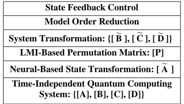
[image:2.612.98.278.227.329.2]Figure 1 illustrates the layout of the closed-system quantum computing control methodology which is used in this paper.
Figure 1. The introduced control methodology which is utilized for
closed quantum computing systems.
In Figure 1, Layer 1 is the closed-system quantum computing model using the time-independent Schrödinger equation (TISE). Layer 2 is the neural network identification of the transformed system matrix [A~ ]. Layer 3 is the LMI
technique used in determining the permutation matrix which is required for system transformation {[B~], [C~ ], [D~]}.
Layer 4 is the system transformation. Layer 5 presents the model order reduction. Finally, layer 6 presents the state feedback control.
Section 2 presents background on quantum computing, recurrent supervised neural networks, linear matrix inequality, model transformation, and model order reduction. Section 3 presents a detailed illustration of the recurrent neural network identification with the LMI optimization technique for model order reduction of the quantum computing system. An implementation of the neural network identification with the LMI optimization to the model order reduction of the time-independent quantum computing system is presented in Section 4. Section 5 presents the application of state feedback controller on the reduced order model of the quantum computing system. Conclusion is presented in Section 6. 2. BACKGROUND
This section presents important background on quantum computing systems, supervised neural networks, LMI and model order reduction that will be used in Sections 3, 4 and 5.
2.1
. Quantum Computing
Quantum computing is a method of computation that uses the dynamic process which is governed by the Schrödinger equation [1,12,13,27,28]. The one-dimensional time-dependent Schrödinger equation (TDSE) is as follows:
t h
i V x m h
∂ ∂ =
+ ∂ ∂
− π ψ ψ ( /2π) ψ
2 ) 2 / (
2 2 2
(1)
t h
i H
∂ ∂
= π ψ
ψ ( /2 )
or (2) where h is Planck constant (6.626⋅10-34 J⋅s = 4.136⋅10-15 eV⋅s), V(x, t) is the applied potential, m is the particle mass, i is the imaginary number, ψ(x,t) is the quantum state, H is the Hamiltonian operator where H = - [(h/2π)2/2m]∇2 + V, and ∇2 is the Laplacian operator.
State Feedback Control
Model Order Reduction
System Transformation: {[B~], [ C ], [~ D~]} LMI-Based Permutation Matrix: [P]
Neural-Based State Transformation: [A~ ] Time-Independent Quantum Computing
System: {[A], [B], [C], [D]}
A general solution to TDSE is the expansion of a stationary (time-independent or spatial) basis functions (i.e., eigen states) Ue(rr) using time-dependent (i.e., temporal) expansion coefficients ce(t) as follows:
∑ = =
Ψ n
e
r e u t e c t
r
0
) ( ) ( )
,
(r r
The expansion coefficients ce(t) are a scaled complex
exponentials as follows:
t h
E i e e
e
e k t
c ()= −( /2π)
where Ee are the energy levels.
While the above holds for all physical systems, in quantum computing, the time-independent Schrödinger equation (TISE) is normally used [1,27]:
ψ
π
ψ ( )
) 2 / (
2
2
2 V E
h
m −
=
∇ (3) where the solution ψ is an expansion over orthogonal basis states φi defined in a linear complex vector space called Hilbert space Η as:
=
∑
i i i
c φ
ψ (4) where the coefficients ciare called probability amplitudes and
|ci|2 is the probability that the quantum state ψ will collapse
into the (eigen) state φi . The probability is equal to the inner product φi|ψ 2, with the unitary condition ∑|ci|2 = 1. In
quantum computing, a linear and unitary operator ℑ is used to transform an input vector of quantum bits (qubits) into an output vector of qubits. In two-valued quantum computing, the qubit is a vector of bits which is defined as follows:
⎥
⎦ ⎤ ⎢ ⎣ ⎡ = ≡ ⎥
⎦ ⎤ ⎢ ⎣ ⎡ = ≡
1 0 1 qubit , 0 1 0
computational basis states
{
0,1}
, one has the following quantum state:ψ =α0 +β1 (6) where αα* = |α|2 = p
0 ≡ the probability of having state ψ in state 0 , ββ* = |β|2 = p
1 ≡ the probability of having state ψ in state 1 , and |α|2 + |β|2 = 1. The calculation in quantum computing for multiple systems (e.g., the equivalent of a register) follow the tensor product (⊗). For example, given states ψ1 and ψ2 , one has:
(
) (
)
11 10
01 00
1 0 1
0
2 1 2
1 2
1 2
1
2 2 1
1
2 1 2 1
β β α
β β
α α
α
β α β
α
ψ ψ ψ ψ
+ +
+ =
+ ⊗ + =
⊗ =
(7)
A physical system (e.g., the hydrogen atom) that is described by the following Equation:
ψ =c1Spinup +c2Spindown (8) can be used to physically implement a two-valued quantum computing. Another common alternative form of Equation (8) is as follows:
2 1 2
1
2
1+ + −
=c c
ψ (9) Many-valued (m-valued) quantum computing can also be performed. For the three-valued quantum computing, the qubit becomes a 3-dimensional vector quantum discrete digit (qudit), and in general, for m-valued quantum computing the qudit is of dimension “many” [1,27]. For example, one has for the 3-state quantum computing (in the Hilbert space H) the
following qudits:
⎥ ⎥ ⎥ ⎦ ⎤
⎢ ⎢ ⎢ ⎣ ⎡ = ≡ ⎥ ⎥ ⎥ ⎦ ⎤
⎢ ⎢ ⎢ ⎣ ⎡ = ≡ ⎥ ⎥ ⎥ ⎦ ⎤
⎢ ⎢ ⎢ ⎣ ⎡ = ≡
1 0 0 2 qudit , 0 1 0 1 qudit , 0 0 1 0
qudit0 1 2 (10)
A three-valued quantum state is a superposition of three quantum orthonormal basis states (vectors). Thus, for the orthonormal computational basis states
{
0,1,2}
, one has the following quantum state:2 1
0 β γ
α
ψ = + +
where αα* = |α|2 = p
0 ≡ the probability of having state ψ in state 0 , ββ* = |β|2 = p
1 ≡ the probability of having state ψ in state 1 , γγ* = |γ|2 = p
2 ≡ the probability of having state
ψ in state 2 , and |α|2 + |β|2 + |γ|2 = 1.
The calculation in quantum computing for m-valued multiple systems follow the tensor product in a manner similar to the one demonstrated for the higher-dimensional qubit in the two-valued quantum computing.
Several quantum computing systems were used to implement quantum gates from which complete quantum circuits and systems were constructed [1,7,11,15,26,27], where several of the two-valued and m-valued quantum circuit implementations use the two-valued and m-valued quantum Swap-based and Not-based gates [1,27]. This can be
important, since the Swap and Not gates are basic primitives in quantum computing from which many other gates are built, such as [1,7,11,15,26,27]: (1) two-valued and m-valued Not gate, (2) two-valued and m-valued Controlled-Not gate (i.e., Feynman gate), (3) two-valued and m-valued Controlled-Controlled-Not gate (i.e., Toffoli gate), (4) two-valued and m -valued Swap gate, and (5) two--valued and m-valued Controlled-Swap gate (i.e., Fredkin gate).
For example, it has been shown that a physical system
comprising trapped ions under multiple-laser excitations can be used to reliably implement m-valued quantum computing [11,26]. A physical system in which an atom (or in general a particle) is exposed to a specific potential field (i.e., potential function) can also be used to implement m-valued quantum computing from which the two-valued being a special case [1,27] where the distinct energy states are used as the
normal basis states. ortho
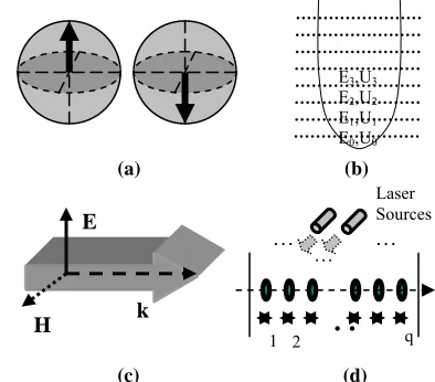
Figure 2 shows several various physical realization methodologies for the implementation of two-valued and m -valued quantum computing [1,7,11,13-15,17,26,27] where Figure 2a shows the particle spin (i.e., the angular momentum) for two-valued quantum computing, Figure 2b shows energy states of quantum systems such as the simple harmonic oscillator potential or the particle in finite-walled box potential for two-valued and m-valued quantum computing in which the resulting distinct energy states are used as the orthonormal basis states, Figure 2c shows light polarization for two-valued quantum computing, and Figure 2d shows cold trapped ions for two-valued and m-valued quantum computing.
E3,U3
E2,U2
E1,U1
E0,U0
(a) (b)
(c) (d)
Figure 2. Various technologies that are used to perform quantum
computing.
In general, for an m-valued logic, a quantum state is a superposition of m quantum orthonormal basis states (i.e., vectors). Thus, for the orthonormal computational basis states
{
0,1,..., m−1}
, one has the following quantum state:
∑
−= = 1
0
m
k k
k q
c
ψ (11)
k E
H
…
… …
…
Laser Sources
q
[image:3.612.338.535.401.574.2]where 1
1
0 2 1
0
*=
∑
=∑
−= −
=
m
k k m
k k
kc c
c . The calculation in quantum
computing for m-valued multiple systems follow the tensor product in a manner similar to the one used for the case of two-valued quantum computing.
Example 1 shows the implementation of m-valued quantum computing by exposing a particle to a potential field U0 where the distinct energy states are utilized as the orthonormal basis states.
Example 1. We assume the following constraints [12,28]: (1)
finite-walled box potential of specific width (L) and height (U0) (i.e., the applied potential value), (2) particle mass m, and (3) boundary conditions for the wavefunction continuity. For the finite potential well, the solution to the Schrödinger equation gives a wavefunction with an exponentially decaying penetration into the classicallly forbidden region where confining a particle to a smaller space requires a larger confinement energy. Since the wavefunction penetration effectively “enlarges the box”, the finite well energy levels are lower than those for the case of infinite well. For a potential which is zero over a length L and has a finite value for other values of x, the solution to the Schrödinger equation has the form of the free-particle wavefunction for (-L/2 < x < L/2) and elsewhere must satisfy the equation:
) ( ) ( ) (
2 2 0
2 2
x U E x
x
m ∂ = − Ψ
Ψ ∂ −h
where h=
(
h/2π)
is the reduced Planck constant. With the following substitution:2 2 2
0 )
( 2
k E
U m
− = −
= β
α
h
the TISE may be written in the form: ) ( )
( 2 2 2
x x
x = Ψ
∂ Ψ
∂ α
and the general solution is in the form: x
x De
Ce
x = α + −α Ψ( )
Given a potential well as shown in Figure 3 and a particle of energy less than the height of the well, the solutions may be of either odd or even parity with respect to the center of the well [12,28]. The Schrödinger equation gives trancendental forms for both so that numerical solution methods must be used. For the even case, one obtains the solution in the form
2 2
2
tankL k
k = −
= β
α . Since both sides of the equation are dependent on the energy E for which one is solving, the equation is trancendental and must be solved numerically. The standard constraints on the wavefunction require that both the wavefunction and its derivative be continuous at any boundary. Applying such constraints is often the way that the solution is forced to fit the physical situation. The ground state solution for a finite potential well is the lowest even parity state and can be expressed in the form:
) 2 / tan(kL k
=
α
where . On the other hand, for the odd case, one obtains the solution in the form
) 2 / ( 2k2 m E= h
2 2
2 tan
k kL
k = −
−
= β
α .
In the one-dimensional case, parity refers to the “evenness” or “oddness” of a function with respect to the reflection about x = 0, where even parity requires
) ( ) (x =Ψ −x
Ψ and odd parity requires Ψ(x)=−Ψ(−x). The stated particle in a box problem can give some insight into the importance of parity in quantum mechanics; the box has a line of symmetry down the center of the box (x = 0) where the basic considerations of symmetry demand that the probability for finding the particle at -x be the same as that at x. Thus, the condition on the probability is given by:
) ( ) ( ) ( )
(xΨ x =Ψ −x Ψ −x
Ψ∗ ∗
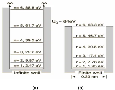
This condition is satisfied if the parity is even or odd, but not if the wavefuntion is a linear combination of even and odd functions. This can be generalized to the statement that wavefunctions must have a definite parity with respect to symmetry operations in the physical problem [12,28]. An example for the distribution of energy states for the particle in finite-walled box is shown in Figure 3.
[image:4.612.325.546.328.501.2](a) (b)
Figure 3. Energy levels and wavefunctions of the one-dimensional
particle in finite-walled box with potential U(x) and the associated energy levels En in electron Volts where, as an example, the energy
levels for an electron in a potential well of depth U0 = 64 eV and
width L = 0.39 nm are shown in comparison with the energy levels of an infinite well of the same size.
0
k
w
1
k
w
2
k
w
∑
ϕ
(
•)
k
y
1
x
2
x
p
x
Output Activation Function
Summing Junction
Synaptic Weights Input
Signals
k
v
Threshold
k
θ kp
w
0
x
Z-1 g1:
A11 A12
A21
A22
B11
B21
) 1 ( ~
1 k+ x
System external input
System Dynamics
Neuron
Delay
Z-1
Outputs
~y(k)
) 1 (
7
) ( ~
1k x
System state: internalinput input 2.2. Recurrent Supervised Neural Networks
2.2. Recurrent Supervised Neural Networks
~ 2 k+ x
) ( ~
2 k x
4
4 8
4
4
6
∑
= =
p
j
j kj
k w x
v 1
⎥ ⎦ ⎤ ⎢
⎣ ⎡ =
22 21
12 11 ~
A A
A A
Ad ⎥
⎦ ⎤ ⎢ ⎣ ⎡ =
21 11 ~
B B Bd
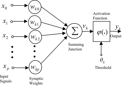
An artificial neural network is an emulation of a biological neural system. The basic model of the neuron is based on the functionality of the biological neuron which is the basic signaling unit in the nervous system. The process of a neuron can be formally modeled as shown in Figure 4 [19,32]. An artificial neural network is an emulation of a biological neural system. The basic model of the neuron is based on the functionality of the biological neuron which is the basic signaling unit in the nervous system. The process of a neuron can be formally modeled as shown in Figure 4 [19,32].
[image:5.612.317.551.90.273.2]
Figure 4. A mathematical model of an artificial neuron.
Figure 4. A mathematical model of an artificial neuron.
As seen in Figure 4, the internal activity of the neuron can be shown to be:
As seen in Figure 4, the internal activity of the neuron can be shown to be:
(12)
∑
(12)= =
p
j
j kj
k w x
v 1
In supervised learning, it is assumed that at each instant of time when the input is applied, the desired response of the system is available. The difference between the actual and the desired response represents an error measure and is used to correct the network parameters externally. Since the adjustable weights are initially assumed, the error measure may be used to adapt the network's weight matrix [W]. A set
of input and output patterns which is called a training set is required for this learning mode. The training algorithm estimates directions of the negative error gradient and then reduces the error.
For artificial neural networks, there are several learning rules used to train the neural network. For example, in the Perceptron learning rule, the learning signal is the difference between the desired and the actual neuron's response (i.e., supervised learning). Another learning rule is the Widrow-Hoff learning rule which minimizes the squared error between the desired output and the neuron's activation value. Backpropagation is also one of the important learning algorithms in neural networks [19,32].
For artificial neural networks, there are several learning rules used to train the neural network. For example, in the Perceptron learning rule, the learning signal is the difference between the desired and the actual neuron's response (i.e., supervised learning). Another learning rule is the Widrow-Hoff learning rule which minimizes the squared error between the desired output and the neuron's activation value. Backpropagation is also one of the important learning algorithms in neural networks [19,32].
The supervised recurrent neural network which is used for the identification in this paper is based on an approximation of the method of steepest descent [19,32]. The network tries to match the output of certain neurons to the desired values of the system output at specific instant of time. Figure 5 shows a network consisting of a total of N neurons with M external input connections for a 2nd order system with two neurons and one external input, where the variable g(k)
denotes the (M x 1) external input vector applied to the
network at discrete time k and the variable y(k + 1) denotes
the corresponding (N x 1) vector of individual neuron outputs produced one step later at time (k + 1).
[image:5.612.71.283.135.286.2]
Figure 5. The utilized second order recurrent neural network
architecture, where the estimated matrices are given by
{ , } and
Figure 5. The utilized second order recurrent neural network
architecture, where the estimated matrices are given by
{ ⎥ , } and
⎦ ⎤ ⎢
⎣ ⎡ =
22 21
12 11 ~
A A
A A
Ad ⎥
⎦ ⎤ ⎢ ⎣ ⎡ =
21 11 ~
B B
Bd W=
[
[A~d] [B~d]]
.The input vector g(k) and one-step delayed output vector y(k) are concatenated to form the ((M + N) x 1) vector u(k),
whose ith element is denoted by u
i(k). IfΛ denotes the set of
indices i for which gi(k) is an external input, and denotes
the set of indices i for which u
ß
i(k) is the output of a neuron
(which is yi(k)), the following is true:
⎪⎩ ⎪ ⎨ ⎧
∈ ∈
β
i , k y
Λ
i , k g = k u
i i i
if ) (
if ) ( )
(
The (N x (M + N)) recurrent weight matrix of the network is represented by the variable [W]. The net internal activity of
neuron j at time k is given by: ) ( ) ( =
)
(k w k u k
v ji i
Λ
i
j
∑
∪
∈ β
where Λ is the union of sets Λand . At the next time step (k + 1), the output of the neuron j is computed by passing v
∪
ß
ß
j(k) through the nonlinearity ϕ(.) obtaining:
)) ( ( = ) 1
(k v k
yj + ϕ j
The derivation of the recurrent algorithm can be started by using dj(k) to denote the desired (i.e., target) response of
neuron j at time k, and to denote the set of neurons that are chosen to provide externally reachable outputs. A time-varying (N x 1) error vector e(k) is defined whose j
) (k
ς
th element is given by the following relationship:
⎪⎩ ⎪ ⎨
⎧ ∈
otherwise
0,
) ( if ), ( ) ( = )
(k d k y k j k
ej j j ς
The objective is to minimize the cost function Etotal which is obtained by:
) ( =
total E k
E k
where ( ) 2
1 = )
(k e2 k
E j
j
∑
∈ς
.
To accomplish this objective, the learning method of steepest descent, which requires knowledge of the gradient matrix, is used:
) ( = ) ( = = total
total E k
k E E E k k W W W
W ∂ ∇
∂ ∂
∂
∇
∑
∑
where is the gradient of E(k) with respect to the weight matrix [W]. In order to train the recurrent network in
real time, the instantaneous estimate of the gradient is used . For the case of a particular weight (k), the incremental change (k) made at time k is defined as:
) (k E
W ∇
(
∇WE(k))
wmll m w ∆ ) ( ) ( -= ) ( k w k E k w m m l l ∂ ∂ ∆ η
where η is the learning-rate parameter. Hence:
) ( ) ( ) ( -= ) ( ) ( ) ( = ) ( ) ( k w k y k e k w k e k e k w k E m i j j m j j j
ml l ∂ l
∂ ∂ ∂ ∂ ∂
∑
∑
∈∈ς ς
To determine the partial derivative , the network dynamics are derived. The derivation is obtained by using the chain rule which provides the following equation:
) ( )/ (k w k yj ∂ ml ∂ ) ( ) ( )) ( ( = ) ( ) ( ) ( 1) + ( = ) ( 1) + ( k w k v k v k w k v k v k y k w k y m j j m j j j m j l l l & ∂ ∂ ∂ ∂ ∂ ∂ ∂ ∂ ϕ where ) ( )) ( ( = )) ( ( k v k v k v j j j ∂ ∂ϕ
ϕ& .
Differentiating the net internal activity of neuron j with respect towml(k) yields:
⎥ ⎥ ⎦ ⎤ ⎢ ⎢ ⎣ ⎡ ∂ ∂ ∂ ∂ ∂ ∂ ∂ ∂
∑
∑
∪ ∈ ∪ ∈ ) ( ) ( ) ( + ) ( ) ( ) ( = ) ( )) ( ) ( ( = ) ( ) ( k u k w k w k w k u k w k w k u k w k w k v i m ji m i ji Λ i m i ji Λ i m j l l l l β βwhere
(
∂wji(k)/∂wml(k))
equals "1" only when j = m and i = ; otherwise, it is "0". Thus:l (k) u δ (k) w (k) u k w k w k v mj m i ji Λ i m j l l l + ∂ ∂ ∂ ∂
∑
∪ ∈ ) ( = ) ( ) ( βwhere is a Kronecker delta equal to "1" when j = m and "0" otherwise, and:
δmj ⎪ ⎩ ⎪ ⎨ ⎧ ∈ ∂ ∂ ∈ ∂ ∂ β i k w k y Λ i k w k u m i m i if , ) ( ) ( if 0, = ) ( ) ( l l
Having those equations produces:
⎥ ⎥ ⎦ ⎤ ⎢ ⎢ ⎣ ⎡ + ∂ ∂ ∂ ∂
∑
∈ ) ( ) ( ) ( ) ( )) ( ( = ) ( 1) + ( k u k w k y k w k v k w k y m m i ji i j m j l l l l & δ ϕ βThe initial state of the network at time k = 0 is assumed to be zero as follows:
0 = ) 0 ( (0) l m i w y ∂ ∂
, for {j∈ ß, m∈ ß, l∈Λ∪β } The dynamical system is described by the following triply indexed set of variables (πmjl):
) ( ) ( = ) ( k w k y k m j j m l l ∂ ∂ π
For every time step k and all appropriate j, m and , system
dynamics are controlled by: l
⎥ ⎥ ⎦ ⎤ ⎢ ⎢ ⎣ ⎡ +
∑
∈ ) ( ) ( ) ( )) ( ( = 1) +(k v k wji k mi k mju k
i j j
ml ϕ& π l δ l
π
β
with j (0)=0.
ml
π
The values of j (k )and the error signal e
ml
π j(k) are used
to compute the corresponding weight changes:
w (k )= ej(k) mj (k) (13) j
m η π
ς l
l
∑
∈
∆
Using the weight changes, the updated weight (k + 1) is
calculated as follows: l
m
w
wml(k+1)=wml(k )+∆wml(k) (14) Repeating this computation procedure provides the minimization of the cost function and the objective is therefore achieved.
With the many advantages that the ANN has, it is used for parameter identification in model transformation for the purpose of model order reduction as will be shown in the following section.
2.3. LMI and Model Transformation
In this sub-section, the detailed illustration of system transformation using LMI optimization will be presented. Consider the system:
x&(t)=Ax(t)+Bu(t) (15) y(t)=Cx(t)+Du(t) (16) In order to determine the transformed [A] matrix, which is
[A~ ], the discrete zero input response is obtained. This is
achieved by providing the system with some initial state values and setting the system input to zero (i.e., u(k) = 0). Hence, the discrete system of Equations (15) - (16), with the initial condition x(0)=x0, becomes:
x(k+1)=Adx(k) (17) y(k)=x(k) (18) We need x(k) as a neural network target to train the network to obtain the needed parameters in [A~d] such that the system
output will be the same for [Ad] and [Ad
~
⎥ (19)
⎦ ⎤ ⎢ ⎣ ⎡ = o c r A A A A 0 ~ Having the [A] and [A~ ] matrices, the permutation [P] matrix is determined using the LMI optimization technique as will be illustrated in later sections. The complete system transformation can be achieved as follows: assuming x P x 1 ~= − , the system of Equations (15) - (16) can be re-written as: ) ( ) ( ~ ) ( ~x t APx t Bu t P& = + ) ( ) ( ~ ) ( ~y t =CPx t +Du t where (~y(t)= y(t)). Pre-multiplying the first equation above by [P-1], one obtains: ) ( ) ( ~ ) ( ~ 1 1 1Px t P APx t P But P− & = − + − ) ( ) ( ~ ) ( ~y t =CPx t +Du t which yields the following transformed model: x~&(t)= A~~x(t)+B~u(t) (20)
~y(t)=C~x~(t)+D~u(t) (21) y (31)
where the transformed system matrices are given by: A~=P−1AP (22)
B~=P−1B (23)
C~=CP (24)
D~=D (25)
Transforming the system matrix [A] into the form shown in Equation (19) can be achieved based on the following definition [22]. Definition.Matrix A∈Mnis reducible if either: (a) n = 1 and A = 0; or (b) n≥ 2, there is a permutation matrix P∈Mn, and there is some integer r with 1≤r≤n−1 such that: ⎥ (26)
⎦ ⎤ ⎢ ⎣ ⎡ = − Z Y X AP P 0 1 where X∈Mr,r, Z∈Mn−r,n−r, Y∈Mr,n−r, and0∈Mn−r,r is a zero matrix. The attractive features of the permutation matrix [P] such as being orthogonal and invertible have made this transformation easy to carry out. However, the permutation matrix structure narrows the applicability of this method to a very limited category of applications. Some form of a similarity transformation can be used to correct this problem; , where is a linear operator defined by [22]. Therefore, based on [A] and [ n n n n R R f : × → ×
f
AP P A f( )= −1 A~], linear matrix inequalities are used to obtain the transformation matrix [P]. Thus, the optimization problem is casted as follows: P−P P− AP−A <ε o p ~ to Subject min 1 (27)which maybe written in an LMI equivalent form as: (28)
0 ) ~ ( ~ 0 ) ( to Subject ) ( trace min 1 1 2 1 > ⎥ ⎥ ⎦ ⎤ ⎢ ⎢ ⎣ ⎡ − − > ⎥ ⎦ ⎤ ⎢ ⎣ ⎡ − − − − I A AP P A AP P I I P P P P S S T T o o S ε where S is a symmetric slack matrix [22]. 2.4. Model Order Reduction Linear time-invariant models of many physical systems have fast and slow dynamics which can be referred to as singularly perturbed systems. Neglecting the fast dynamics of a singularly perturbed system provides a reduced slow model. This gives the advantage of designing simpler lower-dimensionality reduced order controllers based on the reduced model information. To show the formulation of a reduced order system model, consider the singularly perturbed system: x&(t )=A11x(t)+A12ξ(t )+B1u(t), x(0)=x0 (29)
εξ&(t)=A21x(t)+A22ξ(t)+B2u(t), ξ(0)=ξ0 (30)
) ( ) ( ) (t =C1xt +C2ξ t where and are the slow and fast state variables, respectively, and are the input and output vectors, respectively, { , [ ], [ ]} are constant matrices of appropriate dimensions with 1 m x∈ℜ ξ∈ℜm2 1 n u∈ℜ y∈ℜn2 ] [Aii Bi Ci } 2 , 1 { ∈ i , and
ε
is a small positive constant. The singularly perturbed system in Equations (29) - (31) is simplified by setting ε=0. In doing so, we are neglecting the fast dynamics of the system and assuming that the state variablesξ
have reached the quasi-steady state. Hence, setting ε=0 in Equation (30), and assuming [A22] is nonsingular, produces: ξ(t)=−A22−1A21xr(t)−A22−1B1u(t) (32)where the index r denotes remained (or reduced) model. Substituting Equation (32) in Equations (29) - (31) yields the reduced order model: x&r(t) = Arxr(t)+Bru(t) (33)
y(t)=Crxr(t)+Dru(t) (34)
where: Ar = A11−A12A22−1A21 (35)
Br =B1−A12A22−1B2 (36)
Cr =C1−C2A22−1A21 (37)
Dr =−C2A22−1B2 (38)
Example 2. Consider the 3rd order system:
) ( 4 . 0
5 . 1
3 . 1 ) ( 33 20 11
9 26 11
13 9 25 )
(t xt ut
x
⎥ ⎥ ⎥ ⎦ ⎤ ⎢ ⎢ ⎢ ⎣ ⎡ + ⎥ ⎥ ⎥ ⎦ ⎤ ⎢
⎢ ⎢ ⎣ ⎡
− −
− −
=
&
[
1.1 0.4 1.2]
() )(t xt
+
-
1
L
1
R
out
v
a b
in
v
2
L L3
1
C C2 R2 +
-
+
-
1
x x5
2
x 3
x
4
x
Since this is a 3rd order system, there exists three eigenvalues which are {-19.886 + 6.519i, -19.886 - 6.519i, -44.228}. Using the singular perturbation technique, the system model is reduced to the following 2nd order model:
( )
1.609 1.142 )
( 20.546 -14
1.121 29.333
-)
(t x t u t
xr r ⎥
⎦ ⎤ ⎢ ⎣ ⎡ + ⎥ ⎦ ⎤ ⎢
⎣ ⎡ =
&
In order to obtain a state space model for the above system, let the dynamics of the system be designated as system states (xi). This means that there will be a 5th order system since there are five dynamical elements in the system. The model can be obtained by assigning the following set of states {x1 is the current of the inductor L1, is the voltage of the capacitor C
2
x
1, x3 is the current of the inductor L2, is the voltage of the capacitor C
4
x 2, and is the current
of the inductor L
5
x
3}. Applying KCL at nodes (a) and (b) and KVL for the three loops starting from left to right in Figure 7 yields the following state space matrices:
yr(t)=
[
1.5 1.127]
xr(t) +[
0.015]
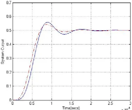
u(t) [image:8.612.60.267.176.335.2]System output response plots of the original system and the reduced model, for a step input, are shown in Figure 6.
Figure 6. Output step response of the original and reduced order models ( ___ original, -.-.-. reduced).
It is seen from the results obtained in Figure 6 that the reduced order model is performing well as compared with the original system response.
Dynamic systems with much higher dimensions can also be processed by following the previously used method and the following example illustrates a 5th order RLC system.
Example 3. Consider the following 5th order RLC filter
[image:8.612.75.281.471.537.2]shown in Figure 7 [20].
Figure 7. An example of a 5th order RLC network.
It is well known that the capacitor and the inductor are dynamical passive elements, which means that they have the ability to store energy. The dynamical equations may be derived using the Kirchhoff's current law (KCL) and Kirchhoff's voltage law (KVL) [20]. The current for the capacitor is proportional to the change of its voltage, that is:
dt t dv C t
i i
i
c i c
) ( )
( =
and that the voltage across the inductor is proportional to the change of its current, that is:
dt t di L t
v i
i
L i L
) ( )
( =
⎥ ⎥ ⎥ ⎥ ⎥ ⎥ ⎥ ⎥ ⎥ ⎥ ⎥ ⎥ ⎥
⎦ ⎤
⎢ ⎢ ⎢ ⎢ ⎢ ⎢ ⎢ ⎢ ⎢ ⎢ ⎢ ⎢ ⎢
⎣ ⎡
− − − − − −
=
3 2 3 1 0 0 0
2 1 0 2 1 0 0
0 2 1 0 2 1 0
0 0 1 1 0 1 1
0 0 0 1 1 1 1
L R L
C C
L L
C C
L L R
A ,
⎥ ⎥ ⎥ ⎥ ⎥ ⎥ ⎥ ⎥
⎦ ⎤
⎢ ⎢ ⎢ ⎢ ⎢ ⎢ ⎢ ⎢
⎣ ⎡
=
0 0 0 01 1
L
B ,
[0 0 0 0 R2]
C= , D=[ ]0
Given the following set of values {C1=C2=2nF, H
11
3
1=L = µ
L , L2=33µH, R1=R2=93Ω}, the corresponding 5th order model is obtained. The eigenvalues of the system are found to be 1⋅106 x {-2.0158 + 7.3391i, -2.0158 - 7.3391i, -4.4229, -4.2273 + 5.2521i, -4.2273 - 5.2521i}. Performing model reduction, the system is reduced from its 5th order to a 4th order by taking the first four rows of [A] as the first category represented by Equation (29) and
taking the fifth row of [A] as the second category represented
by Equation (30). Simulations of both, the original and the reduced models, are shown in Figure 8.
[image:8.612.322.541.497.679.2]As can be observed from the results shown in Figure 8, the reduced order model using the singular perturbation method has provided an acceptable response when compared with the original system response.
3. NEURAL IDENTIFICATION WITH LMI
OPTIMIZATION FOR THE CLOSED-SYSTEM QUANTUM COMPUTING MODEL REDUCTION
In this work, it is our objective to search for a similarity transformation that can be utilized within the context of closed time-independent quantum computing systems to decouple a pre-selected eigenvalue set from the system matrix [A]. To achieve this objective, training the neural network to
estimate the transformed discrete system matrix [Ad
~ ] is performed [5]. For the system of Equations (29) - (31), the discrete model of the quantum computing system is obtained as follows:
x(k+1)= Adx(k)+Bdu(k) (39) y(k)=Cdx(k)+Ddu(k) (40) The estimated discrete model of Equations (39) - (40) can be written in a detailed form as:
( )
) ( ~
) ( ~
) 1 ( ~
) 1 ( ~
21 11
2 1
22 21
12 11
2
1 uk
B B k x
k x A A
A A k
x k x
⎥ ⎦ ⎤ ⎢ ⎣ ⎡ + ⎥ ⎦ ⎤ ⎢ ⎣ ⎡ ⎥ ⎦ ⎤ ⎢
⎣ ⎡ = ⎥ ⎦ ⎤ ⎢
⎣ ⎡
+ +
(41)
⎥
⎦ ⎤ ⎢ ⎣ ⎡ =
) ( ~( ) ~ ) ( ~
2 1
k x
k x k
y (42)
where k is the time index, and the matrix elements of Equations (41) - (42) were shown in Figure 5.
The recurrent neural network presented in Section 2.2 can be summarized by defining Λ as the set of indices i for which is an external input, which in the quantum computing system is one external input and by defining ß as the set of indices i for which is an internal input or a neuron output, which in the quantum computing system is two internal inputs (i.e., two system states). Also, by defining as the combination of the internal and external inputs for which Λ. Using this setting, training the network depends on the internal activity of each neuron which is given by the following equation:
) (k gi
) (k yi
) (k ui
∪
∈ß
i
∑
(43) ∪∈
=
β
Λ
i
i ji
j k w k u k
v ( ) ( ) ( )
where wji is the weight representing an element in the system
matrix or input matrix for j∈ß and i∈ß∪Λ such that
[
[A~d] [~Bd]]
=
W . At the next time step (k +1), the output (i.e., internal input) of the neuron j is computed by passing the activity through the nonlinearity φ(.) as follows:
xj(k+1)=ϕ(vj(k)) (44) With these equations, based on an approximation of the method of steepest descent, the network estimates the system matrix [Ad] as illustrated in Equation (17) for zero input response. That is, an error can be obtained by matching a true state output with a neuron output as follows:
) ( ~ ) ( )
(k x k x k
ej = j − j The objective is to minimize the cost function:
∑
=
k
k E Etotal ( )
where
∑
∈
=
ς j
j k
e k
E( ) 21 2( ) and ς denotes the set of indices j for the output of the neuron structure. This cost function is minimized by estimating the instantaneous gradient of E(k) with respect to the weight matrix [W] and then updating [W]
in the negative direction of this gradient. In steps, this may be proceeded as follows:
- Initialize the weights, [W], by a set of uniformly
distributed random numbers. Starting at the instant k = 0, use Equations (43) - (44) to compute the output values of the N neurons (whereN= ß).
- For every time step k and all j∈ß, m∈ß, and
∪
∈ß
l Λ, compute the dynamics of the system which
are governed by the triply indexed set of variables:
⎥ ⎥ ⎦ ⎤ ⎢
⎢ ⎣ ⎡
+ =
+
∑
∈ß i
mj i
m ji j
j
ml(k 1) ϕ&(v (k)) w (k)π l(k) δ ul(k) π
with initial conditions j (0)=0 and
ml
π δml is given by
(
∂wji(k) ∂wml(k))
, which is equal to "1" only when j = m and i=l otherwise it is "0". Notice that for the special case of a sigmoidal nonlinearity in the form of a logistic function, the derivative ϕ&(⋅
) is given by)] 1 ( 1 )[ 1 ( )) (
(vj k =yj k+ −yj k+
ϕ& .
- Compute the weight changes corresponding to the error signal and system dynamics:
∑
∈= ∆
ς π η
j
j m j
m k e k k
w l( ) ( ) l( ) (45) - Update the weights in accordance with:
wml(k+1)=wml(k)+∆wml(k) (46) - Repeat the computation until the desired identification is
achieved.
As was illustrated in Equations (17) - (18), for the purpose of estimating only the transformed system matrix [A~ ], the
training is based on the zero input response. Once the training is complete, the obtained weight matrix [W] is the discrete
estimated transformed system matrix. Transforming the estimated system back to the continuous form yields the desired continuous transformed system matrix [A~ ]. Using the
LMI optimization technique illustrated in Section 2.3, the permutation matrix [P] is determined. Hence, a complete
system transformation, as was shown in Equations (20) - (21), is achieved. To perform the order reduction, the system in Equations (20) - (21) are written as:
() (47) )
( ~() ~ 0
) ( ~() ~
t u B B t x
t x A A A t x
t x
o r
o r
o c r
o r
⎥ ⎦ ⎤ ⎢ ⎣ ⎡ + ⎥ ⎦ ⎤ ⎢ ⎣ ⎡ ⎥ ⎦ ⎤ ⎢
⎣ ⎡ = ⎥ ⎥ ⎦ ⎤ ⎢ ⎢ ⎣ ⎡
& &
[
]
()) ( ~() ~ )
( ~ () ~
t u D D t x
t x C C t y
t y
o r
o r o r o
r
⎥ ⎦ ⎤ ⎢ ⎣ ⎡ + ⎥ ⎦ ⎤ ⎢ ⎣ ⎡ =
⎥ ⎦ ⎤ ⎢ ⎣ ⎡
0 0.1 0.2 0.3 0.4 0.5 0
0.01 0.02 0.03 0.04 0.05 0.06 0.07 0.08
Time[s]
S
y
s
tem
O
u
tput
where the system transformation enables us to decouple the original system into retained (r) and omitted (o) eigenvalues. The retained eigenvalues are the dominant eigenvalues that produce the slow dynamics and the omitted eigenvalues are the non-dominant eigenvalues that produce the fast dynamics. Equation (47) maybe written as:
) ( ) ( ~ ) ( ~ ) (
~x t Ax t Ax t But r o c r r
r = + +
&
) ( ) ( ~ ) (
~ t A x t B ut
x&o = o o + o
The coupling termAc~xo(t) maybe compensated for by solving for ~xo(t) in the second equation above by setting ~x&o(t) to zero using the singular perturbation method (by settingε=0). Doing so, the following is obtained:
~xo(t)=−Ao−1Bou(t) (49) Using ~xo(t), we get the reduced model given by:
~x&r(t)=Arx~r(t)+[−AcAo−1Bo+Br]u(t) (50) y(t)=Cr~xr(t)+[−CoAo−1Bo+D]u(t) (51) Hence, the overall reduced order model is:
~x&r(t) =Aor~xr(t)+Boru(t) (52) y(t)=Corx~r(t)+Doru(t) (53) where the detail of the {[ ], [ ], [ ], [ ]} overall reduced matrices are shown in Equations (50) - (51).
or
A Bor Cor Dor
Example 4. Consider the 3rd order system:
[
]x
y
u x
x
1 2 . 0 1
5 . 0
1 1
40 5 2
4 30 8
18 5 20
=
⎥ ⎥ ⎥
⎦ ⎤
⎢ ⎢ ⎢
⎣ ⎡ + ⎥ ⎥ ⎥
⎦ ⎤
⎢ ⎢ ⎢
⎣ ⎡
− −
− −
= &
Since the system is a 3rd order, there are three eigenvalues which are {-25.2822, -22, -42.717}. After performing the proper transformation and training, the following desired diagonal transformed model is obtained:
[
] [
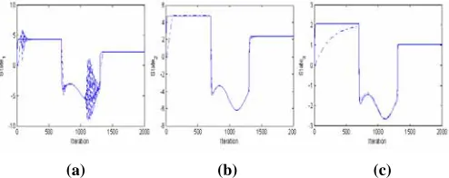
This transformed model was simulated with an input signal that has different functions to capture most of the system dynamics as seen in the state response of Figure 9 which presents the system states while training and converging.
[image:10.612.67.279.467.524.2](a) (b) (c)
Figure 9. System state response for the three states for a sequence of inputs (1) step, (2) sinusoidal, and (3) step ( ___original state. -.-.-.-.- state while convergence).
It is important to notice that the eigenvalues of the original system are preserved in the transformed model as seen in the above diagonal system matrix. Reducing the 3rd order transformed model to a 2nd order model yields:
[
]
x[
uy
u x
x
r r
r r
0.0195
0.1856 1.0405
1.0482 0.5979 22
0
10.4534 25.2822
-+ =
⎥ ⎦ ⎤ ⎢ ⎣ ⎡ + ⎥ ⎦ ⎤ ⎢
⎣ ⎡
− =
&
]
]
with the dominant eigenvalues (slow dynamics) preserved as desired. However, by comparing this transformation-based reduction to the model reduction result of the singular perturbation without transformation (reduced 2nd order model) which is:
[
]
x[
uy
u x
x
r r
r r
0.0125
0.325 1.05
1.05 0.775 29.5
-8.2
2.75 20.9
-+ =
⎥ ⎦ ⎤ ⎢ ⎣ ⎡ + ⎥ ⎦ ⎤ ⎢
⎣ ⎡ =
&
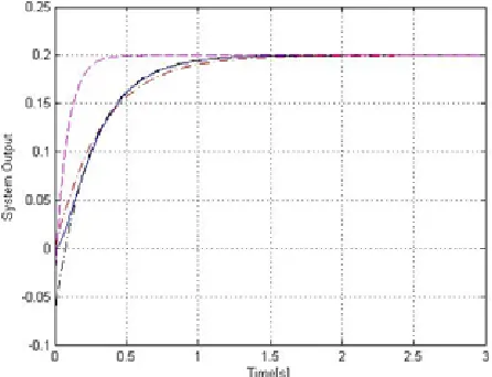
the two eigenvalues {-18.79, -31.60} of the non-transformed reduced model are totally different from the original system eigenvalues. The three different models, the original and the two reduced models (with and without transformation), were tested for a step input signal and the results were obtained as shown in Figure 10.
[image:10.612.53.300.576.674.2]As observed from Example 4, the transformed reduced order model has achieved the two goals of (1) preserving the original system dominant eigenvalues and (2) performing well as compared with the original system response.
Figure 10. Reduced 2nd order models (.… transformed, -.-.-.-
transformed) output responses to a step input along with the non-reduced model ( ____ original) 3rd order system output response.
]
u xy
u x
x
0019 . 0 8581 . 0 1856 . 0 0405 . 1
8777 . 0
7721 . 0
3343 . 0
7178 . 42 0
0
4343 . 13 22 0
8339 . 12 4534 . 0 28221 . 25
+ =
⎥ ⎥ ⎥
⎦ ⎤
⎢ ⎢ ⎢
⎣ ⎡ + ⎥ ⎥ ⎥
⎦ ⎤
⎢ ⎢ ⎢
⎣ ⎡
− − −
= &
4. MODEL REDUCTION OF THE QUANTUM
COMPUTING SYSTEM USING NEURAL IDENTIFICATION AND LMI OPTIMIZATION
The dynamical TISE of the one-dimensional particle in finite-walled box potential V is expressed as follows:
0 ) ( ) 2 / ( 2 2 2 2 = Ψ − + ∂ Ψ ∂ V E h m x π
which also can be written as:
Ψ − = ∂ Ψ ∂ ) ( 2 2 2 2 E V m x h
where m is the particle mass, and h=(h/2π) is the reduced Planck constant (which is also called the Dirac constant) ≅ 1.055⋅10-34 J⋅s = 6.582⋅10-16 eV⋅s. Thus, for
⎪⎭ ⎪ ⎬ ⎫ ⎪⎩ ⎪ ⎨ ⎧ ∂ Ψ ∂ = ′ = ′ ∂ Ψ ∂ = Ψ
= 2 1 2 2 22
1 ,x ,x x ,x
x
x
x , the state space
model of the time-independent closed quantum computing system is given as:
u 0 0 x x 0 ) (
2 0 1 x x 2 1 2 2 1 ⎟⎟ ⎠ ⎞ ⎜⎜ ⎝ ⎛ + ⎟⎟ ⎠ ⎞ ⎜⎜ ⎝ ⎛ ⎥ ⎥ ⎦ ⎤ ⎢ ⎢ ⎣ ⎡ − = ⎟ ⎟ ⎠ ⎞ ⎜ ⎜ ⎝ ⎛ ′ ′ h E V
m (54)
(
)
( )
0u (55) x x 0 1 y 2 1 + ⎟⎟ ⎠ ⎞ ⎜⎜ ⎝ ⎛ =For simulation reasons, Equations (54) – (55) can also be re-written equivalently as follows:
u 0 0 x x -0 1 ) ( 2 0 x x -1 2 2 1 2 ⎟⎟ ⎠ ⎞ ⎜⎜ ⎝ ⎛ + ⎟⎟ ⎠ ⎞ ⎜⎜ ⎝ ⎛ ⎥ ⎥ ⎦ ⎤ ⎢ ⎢ ⎣ ⎡ − − = ⎟ ⎟ ⎠ ⎞ ⎜ ⎜ ⎝ ⎛ ′ ′ h V E m (56)
(
)
( )
0u (57) x x -1 0 y 1 2 + ⎟⎟ ⎠ ⎞ ⎜⎜ ⎝ ⎛ =Also, for conducting the simulations, one may often need to scale system Equation (56) without changing the system dynamics. Thus, by scaling both sides of Equation (56) by a scaling factor a, the following set of equations is obtained:
u 0 0 x x -0 1 ) ( 2 0 x x -1 2 2 1 2 ⎟⎟ ⎠ ⎞ ⎜⎜ ⎝ ⎛ + ⎟⎟ ⎠ ⎞ ⎜⎜ ⎝ ⎛ ⎥ ⎥ ⎦ ⎤ ⎢ ⎢ ⎣ ⎡ − − = ⎟ ⎟ ⎠ ⎞ ⎜ ⎜ ⎝ ⎛ ′ ′ h V E m a
a (58)
(
)
( )
0u (59) x x -1 0 y 1 2 + ⎟⎟ ⎠ ⎞ ⎜⎜ ⎝ ⎛ =Therefore, one obtains the following set of time-independent quantum system matrices:
A = ⎥ ⎥ ⎦ ⎤ ⎢ ⎢ ⎣ ⎡ − − 0 1 ) ( 2 0 2 h V E m
a (60)
B = ⎥ (61)
⎦ ⎤ ⎢ ⎣ ⎡ 0 0
C =
[
0 1]
(62) D =[ ]
0 (63) The specifications of the system matrix in Equation (60) for the particle in finite-walled box are determined by (1) potential box width L (in nano meter), (2) particle mass m, and (3) the potential value V (i.e., potential height in electron Volt). As an example, consider the particle in finite-walledpotential with specifications of (E – V) = 88 MeV and a very light particle with mass of N = 10-33 of the electron mass (where the electron mass me ≅ 9.109⋅10-27 g = 5.684⋅10-12
eV/(m/s)2). This system was discretized using the sampling rate Ts = 0.005 second and simulated for a zero input. Hence,
based on the obtained simulated output data and using NN to estimate the subsystem matrix [Ac] of Equation (19) with learning rate η = 0.015, the following transformed system matrix [A~ ] was obtained:
A~ = ⎥
⎦ ⎤ ⎢ ⎣ ⎡ o c r A A A 0
where [Ar] is set to provide the dominant eigenvalues (slow dynamics) and [Ao] is set to provide the non-dominant eigenvalues (fast dynamics) of the original system. Thus, when training the system, the second state ~xo(t) of the transformed model in Equation (47) is unchanged due to the restriction of [0 Ao] seen in [A~ ]. This may lead to an
undesired starting of the system response, but fast system overall convergence.
Using [A~ ] along with[A], the LMI is then implemented
in order to obtain {[B~], [C~], [D~]} which makes a complete
model transformation. Finally, by using the singular perturbation technique for model order reduction, the reduced order model is obtained.
Thus, by the implementation of the previously stated system specifications and using the squared reduced Planck constant of 2 = 43.324 ⋅ 10
h -32 (eV⋅s)2, one obtains the following scaled system matrix from Equation (60):
⎥ ⎦ ⎤ ⎢ ⎣ ⎡ − − ⎟ ⎠ ⎞ ⎜ ⎝ ⎛ − = ⎥ ⎥ ⎦ ⎤ ⎢ ⎢ ⎣ ⎡ − ⋅ ≅ ⎥ ⎥ ⎦ ⎤ ⎢ ⎢ ⎣ ⎡ − − = − − 16 9 . 4761 0116 . 0 0 5000 1 003 . 0 95 . 0 10 32 . 2 0 0 1 ) ( 2
0 2 6
1 h V E m A a
for which the system simulations were performed for . Accordingly, the eigenvalues were found to be {-5.0399, -10.9601}.
⎥ ⎦ ⎤ ⎢ ⎣ ⎡ − − = 16 9 . 4761 0116 . 0 0 A
The investigation of the proposed method of system modeling for the closed quantum computing system using neural network with LMI and model order reduction was tested on a PC platform with hardware specifications of Intel Pentium 4 CPU 2.40 GHz, and 504 MB of RAM, and software specifications of MS Windows XP 2002 OS and Matlab 6.5 simulator.