Transformation Methods for the Blasius Problem and its Recent Variants

Transformation Methods for the Blasius Problem

and its Recent Variants

Riccardo Fazio

∗

Abstract—Blasius problem is the simplest nonlin-ear boundary layer problem. We hope that any ap-proach developed for this epitome can be extended to more difficult hydrodynamics problems. With this motivation we review the so called T¨opfer transfor-mation, which allows us to find a non-iterative nu-merical solution of the Blasius problem by solving a related initial value problem and applying a scaling transformation. The applicability of a non-iterative transformation method to the Blasius problem is a consequence of its partial invariance with respect to a scaling group. Several problems in boundary-layer theory lack this kind of invariance and cannot be solved by non-iterative transformation methods. To overcome this drawback, we can modify the problem under study by introducing a numerical parameter, and require the invariance of the modified problem with respect to an extended scaling group involving this parameter. Then we apply initial value methods to the most recent developments involving variants and extensions of the Blasius problem.

Keywords: boundary-layer theory, scaling invariance, transformation methods, initial value methods.

1

Introduction

At the beginning of the last century L. Prandtl [17] put the foundations of boundary-layer theory providing the basis for the unification of two, at that time seemingly incompatible, sciences: namely, theoretical hydrodynam-ics and hydraulhydrodynam-ics. Boundary-layer theory has found its main application in calculating the skin-friction drag which acts on a body as it is moved through a fluid: for example the drag of an airplane wing, of a turbine blade, or a complete ship [18].

With the turning of this new century, as the num-ber of applications of microelectronics devices increases, boundary-layer theory has found a renewal of interest within the study of gas and liquid flows at the micro-scale regime [6, 16].

∗

Department of Mathematics, University of Messina, Con-trada Papardo, Salita Sperone 31, 98166 Messina, Italy. E-mail: [email protected] Home-page: http://mat520.unime.it/fazio

Acknowledgement. This work was supported by the

Univer-sity of Messina and partially by the Italian MUR. Date of the manuscript submission: February 14, 2008.

Blasius problem is the simplest nonlinear boundary layer problem. A recent study by Boyd pointed out how this particular problem of boundary-layer theory has arose the interest of prominent scientist, like H. Weyl, J. von Neumann, M. Van Dyke, etc., see Table 1 in [4]. The main reason for this interest is due to the hope that any approach developed for this epitome can be extended to more difficult hydrodynamics problems. Our main goal here is to show how to solve numerically the Blasius problem, and its variants and extensions, by initial value methods derived within scaling invariance theory.

2

Fluid flow on a flat plate

The model describing the steady plane flow of a fluid past a thin plate, provided the boundary layer assumptions are verified (v≫wand the existence of a very thin layer attached to the plate), is given by

∂v ∂y +

∂w ∂z = 0

v∂v ∂y+w

∂v ∂z =µ

∂2

v ∂z2

(1)

v(y,0) =w(y,0) = 0

v(y, z)→V∞ as z→ ∞,

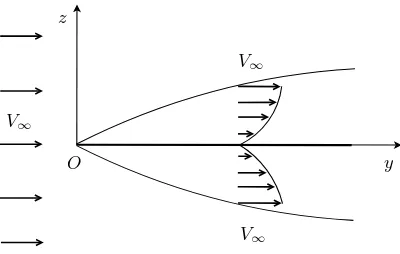
where the governing differential equations, namely con-servation of mass and momentum, are the steady-state 2D Navier-Stokes equations under the boundary layer ap-proximations,vandware the velocity components of the fluid in the y and z direction, V∞ represents the

main-stream velocity, see the draft in figure 1, and µ is the viscosity of the fluid. The boundary conditions atz = 0 are based on the assumption that neither slip nor mass transfer are permitted at the plate whereas the remain-ing boundary condition means that the velocity v tends to the main-stream velocityV∞asymptotically.

In order to study this problem it is convenient to intro-duce a potential (stream function)ψ(y, z) defined by

v= ∂ψ

∂z, w=− ∂ψ

∂y .

y z

O

V∞ V∞

[image:2.595.68.268.70.197.2]

V∞

Figure 1: Boundary layer over a thin plate.

equation of continuity is satisfied identically, and we have to deal only with the transformed momentum equation. In fact, introducing the stream function the problem can be rewritten as follows

µ∂

3

ψ ∂z3 +

∂ψ ∂y

∂2

ψ ∂z2 −

∂ψ ∂z

∂2

ψ ∂y∂z = 0 ∂ψ

∂y(y,0) = ∂ψ

∂z(y,0) = 0 (2) ∂ψ

∂z(y, z)→V∞ as z→ ∞.

2.1

Blasius problem

Blasius [3] introduced the following similarity transfor-mation

η=z

V∞

µy

1/2

, f(η) =ψ(y, z) (µyV∞) −1/2

,

that reduces the partial differential model (2) to

d3

f dη3 +

1 2f

d2

f dη2 = 0

(3)

f(0) = df

dη(0) = 0, df

dη(η)→1 as η→ ∞,

i.e., a boundary value problem (BVP) defined on a semi-infinite interval. Blasius solved this BVP by patching a power series to an asymptotic approximation at some finite value ofη.

2.2

T¨

opfer transformation

By considering the derivation of the series expansion so-lution of the Blasius problem, T¨opfer [20] defined a trans-formation of variables that reduces the BVP into an ini-tial value problem (IVP). However, it is much simpler to consider directly the transformation

f∗

=λ−1/3

f , η∗

=λ1/3η , (4)

and to define the non-iterative transformation method. We notice that the governing differential equation and the initial conditions at the free surface are left invariant

by the new variables defined in (4). Moreover, T¨opfer used the missed initial condition

d2

f∗

dη∗2(0) = 1.

The first and second order derivatives transform in the following way

df∗

dη∗ =λ −2/3df

dη , d2

f∗

dη∗2 =λ

−1d 2

f dη2 ,

and the value of λ can be found on condition that we have an approximation for _dηdf∗∗(∞). In fact, by the first of the above relations we get

λ=

df∗

dη∗(∞)

−3/2

. (5)

Let us list the steps necessary to solve the Blasius problem by the considered approach, we have to:

1. solve the IVP

d3

f∗

dη∗3 + 1 2f

∗d

2

f∗

dη∗2 = 0

(6)

f∗

(0) = df

∗

dη∗(0) = 0,

d2

f∗

dη∗2(0) = 1 and, in particular, get an approximation for df_dη∗∗(∞);

2. computeλby equation (5);

3. obtainf(η) by the inverse transformation of (4).

In this way we have defined an initial value method for the Blasius problem. In literature such a method is also known as a non-iterative transformation method (ITM).

2.3

Truncated boundary approximation

From a numerical point of view the request to evaluate

df

dη(∞) cannot be fulfilled. Several strategies have been

proposed in order to provide an approximation of this value. The simplest and widely used one is to introduce, instead of infinity, a suitable truncated boundary η∞.

The question on how to set a satisfactory value of η∞

is not addressed in this work. A recent successful way to deal with such a question is to reformulate the consid-ered problem as a free BVP [8, 9, 10]. For instance, as far as the Blasius problem is concerned, we can replace the asymptotic condition with the free boundary conditions

df

dη(ηǫ) = 1, d2

f

dη2(ηǫ) =ǫ (7)

whereηǫis the unknown free boundary and 0≤ǫ≪1 is

For the sake of simplicity we will not use the free bound-ary approach here, but we perform some preliminbound-ary computational tests in order to find a suitable value for the truncated boundaryη∞.

[image:3.595.68.270.172.342.2]

2.4

Numerical results

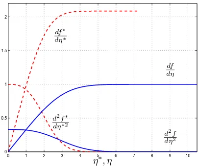
Figure 2 shows a sample numerical computation. We

0 1 2 3 4 5 6 7 8 9 10

0 0.5 1 1.5 2

η∗

, η

df∗

dη∗

df dη

d2_f∗

dη∗2

d2_f

dη2

Figure 2: Blasius solution by a non-ITM.

used a variable step-size classical fourth order Runge-Kutta method, implemented in order to maintain a local error of the order of 10−6

. Moreover, the calculation were performed in the starred variables with a first time step equal to 0.1 and η∗

∞ = 7.25. The asymptotic value of

interest was found to be

df∗

dη∗(∞)≈2.085409.

This value can be used in equation (5) to get

d2

f

dη2(0)≈0.332057.

Blasius solution was found by rescaling.

2.5

The iterative transformation method

The applicability of a non-ITM to the Blasius problem is a consequence of its partial invariance with respect to the transformation (4); the asymptotic boundary condition is not invariant. Several problems in boundary-layer theory lack this kind of invariance and cannot be solved by non-ITMs. To overcome this drawback, we can modify the problem under study by introducing a numerical param-eterh, and require the invariance of the modified problem with respect to an extended scaling group involvingh, see [11] for details.

An ITM can be defined as follows:

1. - the original BVP is embedded into a modified prob-lem involving the numerical parameterh, so that it is

ensured the invariance of the modified problem with respect to an extended scaling group involvingh.

2. - by starting with suitable values ofh∗

0andh

∗

1a root-finder method is used to define a sequence h∗

j, for

j= 2,3, . . . , . At each iteration the group parameter

λ is obtained by solving an IVP numerically. The related sequence Γ(h∗

j),forj= 0,1,2, . . . , is defined

by

Γ(h∗

) =h−1 with h=h(h∗

), (8)

Γ(·) is defined implicitly by the solution of an IVP written in the starred variables and as a consequence

h=h(h∗

) .

3. - suitable termination criteria have to be used to ver-ify whether Γ(h∗

j)→0 asj → ∞.

4. - the solution of the original problem can be obtained by rescaling toh= 1.

By defining an ITM the existence and uniqueness ques-tion can be reduced to finding the number of real zeros of the transformation function Γ(·). This result can be stated as follows.

Theorem 1 Let us assume that IVPs used to define the transformation function are well posed. Then, the consid-ered BVP has a unique solution if and only if the trans-formation function has a unique real zero; nonexistence (nonuniqueness) of the solution is equivalent to nonexis-tence of real zeros (exisnonexis-tence of more than one real zero) of Γ(·).

The underlying idea of the proof of this theorem is that there exists a one-to-one and onto correspondence be-tween the set of solutions of the BVP and the set of real zeros of the transformation function, see [11]. This theo-rem is applied in the next section.

3

Recent developments

In this section we report on recent developments involving some extensions of the Blasius problem and the related numerical approximation. The results reported in this section were found by theode113 solver, from the MAT-LAB ODE suite written by Samphine and Reichelt [19], with the accuracy and adaptivity parameters defined by default.

3.1

Moving surfaces

0 1 2 3 4 5 6 7 8 9 10 −0.4

−0.2 0 0.2 0.4 0.6 0.8 1

η

df dη

d2_f

dη2

0 5 10 15

−0.4 −0.2 0 0.2 0.4 0.6 0.8 1

η

df dη

d2_f

[image:4.595.67.531.72.256.2]

dη2

Figure 3: Blasius problem with moving plate boundary conditions. The two different solutions forP = 0.25.

condition at infinity, and the following non-homogeneous boundary conditions atη= 0

f(0) = 0, df

dη(0) =−P , (9)

whereP is the ratio of the boundary velocity to the free stream velocity. Klemp and Acrivos studied the effect of the parameter P on the boundary layer thickness. For

P >0, two solutions exist only for P less than a critical value Pc, as shown numerically by Hussaini and Lakin

[13]. These authors found a numerical value of Pc equal

to 0.3541. Hussaini et al. [14] proved the nonuniqueness and analyticity of solutions forP ≤Pc, and derived the

upper bound 0.46824 forPc.

More recently, a modified Blasius equation, taking into account the effect ofP on the boundary layer thickness, has been introduced by Allan [1]. Moreover, Allan and Syam [2], using an homotopy analysis method, define an implicit relation between the wall shear stress and the moving wall parameters. The study of these relation shows that two solutions exist whenP ≤Pc ≈0.354. . .,

one solution exists forP =Pc and no solution exists for

P > Pc.

We have used the ITM in order to investigate the exis-tence and uniqueness question for the Blasius model on a moving plate. For the modified problem we defined the boundary condition

df

dη(0) =−h P

and used the extended scaling group

f∗

=λf , η∗

=λ−1

η , h∗

=λ2h . (10)

so thatλis defined by

λ=

_df∗

dη∗(∞)

1/2

. (11)

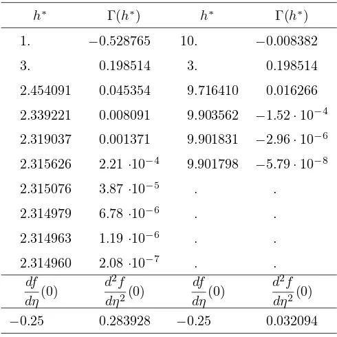
Here we report on sample numerical results. First let us consider the case P = 0.25. Sample numerical results are reported in Table 1. In this case Γ(·) has two

differ-h∗

Γ(h∗

) h∗

Γ(h∗

)

1. −0.528765 10. −0.008382

3. 0.198514 3. 0.198514

2.454091 0.045354 9.716410 0.016266

2.339221 0.008091 9.903562 −1.52·10−4 2.319037 0.001371 9.901831 −2.96·10−6 2.315626 2.21·10−4

9.901798 −5.79·10−8

2.315076 3.87·10−5

. .

2.314979 6.78·10−6

. .

2.314963 1.19·10−6

. .

2.314960 2.08·10−7

. .

df dη(0)

d2

f dη2(0)

df dη(0)

d2

f dη2(0)

−0.25 0.283928 −0.25 0.032094

Table 1: Fluid flow on a moving plate: numerical results by the ITM.

ent zeros. Figure 3 shows the two corresponding solution found by the ITM. It is evident, from the two frames of this figure, that the truncated boundary approach has to be supplemented by some preliminary numerical experi-ments and this is more relevant in the case of non unique-ness of solution. In fact, if we setη∞= 10, then we miss

the solution shown in the right frame of figure 3. For the ITM we used the convergence criterion|Γ(·)|<10−6

[image:4.595.305.550.350.595.2]

such a case.

3.2

Slip flow condition

We consider now the case of a rarefied flow where the no-slip condition at the wall, considered in the previous section, must be replaced by a slip-flow condition, see for instance Gad-el-Hak [6]. For an isothermal wall, the slip condition can be defined as

v(y,0) = 2−σ

σ ℓ ∂v ∂z(y,0),

whereℓis the mean free path, andσis the tangential mo-mentum accommodation coefficient. Within a similarity transformation this slip boundary condition becomes

df

dη(0) =P d2

f dη2(0),

whereP is a non-dimensional parameter, that takes into account the behaviour at the surface, defined by

P =2−σ

σ Kn Re y

1/2

,

where Knand Re are the Knudsen and Reynolds num-bers based on y.

For the Blasius problem with slip condition we imple-mented both the non-ITM and the ITM. In order to ap-ply the non-ITM we had to require thatP is a parameter involved in the scaling invariance, i.e., we defined the ex-tended scaling group

f∗

=λf , η∗

=λ−1

η , P∗

=λ−1

P . (12)

As far as the application of the ITM is concerned, we used a modified problem with the boundary condition

df

dη(0) =h P d2

f dη2(0),

and the extended scaling group

f∗

=λf , η∗

=λ−1

η , h∗

=λ−1

h . (13)

Henceforth, in both cases λ is defined, once again, by equation (11).

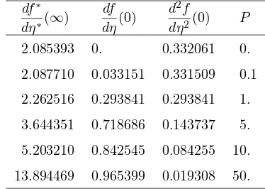
[image:5.595.305.548.70.240.2]

Sample numerical results are reported in Tables 2 and 3. Figure 4 shows a sample numerical integration forP = 1.562257. Note that the solution of the Blasius problem with slip flow condition was computed by rescaling.

For the ITM, we always used h∗

0 = 0.1 and h

∗

1 = 1 but for the caseP = 50 where, in order to speed up the con-vergence, we set h∗

1= 0.5. By setting|Γ(·)|<10

−6 , as a convergence criterion, the Regula Falsi method converged within 8 iterations in all cases.

P∗ df ∗

dη∗(∞)

df dη(0)

d2

f

dη2(0) P

0. 2.085393 0. 0.332061 0.

0.1 2.090453 0.047836 0.330856 0.144584

0.5 2.191907 0.228112 0.308153 0.740255

1. 2.440648 0.409727 0.262266 1.562257

5. 5.771518 0.866323 0.072122 12.011992

10. 10.554805 0.947436 0.029162 32.488159

20. 20.394883 0.980638 0.010857 90.321389

[image:5.595.332.519.273.406.2]

25. 25.353618 0.986053 0.007833 125.880941

Table 2: Non-iterative numerical results.

df∗

dη∗(∞)

df dη(0)

d2

f

dη2(0) P 2.085393 0. 0.332061 0.

2.087710 0.033151 0.331509 0.1

2.262516 0.293841 0.293841 1.

3.644351 0.718686 0.143737 5.

5.203210 0.842545 0.084255 10.

13.894469 0.965399 0.019308 50.

Table 3: Slip boundary condition: numerical results by the ITM.

0 2 4 6 8 10 12

0 0.5 1 1.5 2 2.5

η∗

, η

df∗

dη∗

df dη

d2_f∗

dη∗2

d2_f

dη2

Figure 4: Blasius problem with slip condition. Numerical solution by a non-ITM withP∗

= 1 andP = 1.562257.

4

Future Work

[image:5.595.311.541.453.639.2]

bound-ary conditions

d3

f dη3 +f

d2

f dη2 +β

"

1−

df dη

2#

= 0

(14)

f(0) = df

dη(0) = 0, df

dη(∞) = 1,

where f and η are appropriate similarity variables and

β is a parameter. This problem describes the flow of a fluid past a wedge, see [7]. The application of the ITM to (14) has been reported in [9] but only in the simple case where 0≤β≤1. It is well known that the caseβ >1 is more interesting, because the Falkner-Skan model loses the uniqueness property and a hierarchy of solution with reversed flow exists [5].

References

[1] F. M. Allan. Similarity solutions of a boundary layer problem over moving surfaces. Appl. Math. Letters, 10:81–85, 1997.

[2] F. M. Allan and M. I. Syam. On the analytic so-lutions of the nonhomogeneous Blasius problem. J. Comput. Appl. Math., 182:362–371, 2005.

[3] H. Blasius. Grenzschichten in Fl¨ussigkeiten mit kleiner Reibung. Z. Math. Phys., 56:137, 1908.

[4] J. P. Boyd. The Blasius function in the complex plane. Experimental Math., 8:381–394, 1999.

[5] W. A. Coppel. On a differential equation of boundary-layer theory. Philos. Trans. Roy. Soc. London Ser. A, 253:101–136, 1960.

[6] M. Gad el Hak. The fluid mechanics of microde-vices — the Freeman scholar lecture. J. Fluids Eng., 121:5–33, 1999.

[7] V. M. Falkner and S. W. Skan. Some approximate solutions of the boundary layer equations. Phil. Mag., 12:865–896, 1931.

[8] R. Fazio. The Blasius problem formulated as a free boundary value problem. Acta Mech., 95:1–7, 1992.

[9] R. Fazio. The Falkner-Skan equation: numerical solutions within group invariance theory. Calcolo, 31:115–124, 1994.

[10] R. Fazio. A novel approach to the numerical solu-tion of boundary value problems on infinite intervals.

SIAM J. Numer. Anal., 33:1473–1483, 1996.

[11] R. Fazio. A numerical test for the existence and uniqueness of solution of free boundary problems.

Appl. Anal., 66:89–100, 1997.

[12] R. Fazio. A survey on free boundary identification of the truncated boundary in numerical BVPs on infinite intervals. J. Comput. Appl. Math., 140:331– 344, 2002.

[13] M. Y. Hussaini and W. D. Lakin. Existence and nonuniqueness of similarity solutions of a boundary layer problem. Q. J. Mech. Appl. Math., 39:15–23, 1986.

[14] M. Y. Hussaini, W. D. Lakin, and A. Nachman. On similarity solution of a boundary layer problem with upstream moving wall.SIAM J. Appl. Math., 7:699– 709, 1987.

[15] J. P. Klemp and A. Acrivos. A moving-wall bound-ary layer with reverse flow. J. Fluid Mech., 53:177– 191, 1972.

[16] M. J. Martin and I. D. Boyd. Blasius boundary layer solution with slip flow conditions. InAmerican Institute of Physics Conference Series, volume 585 ofAmerican Institute of Physics Conference Series, pages 518–523, August 2001.

[17] L. Prandtl. ¨Uber Fl¨ussigkeiten mit kleiner Reibung. InProc. Third Intern. Math. Congr., pages 484–494, 1904. Engl. transl. in NACA Tech. Memo. 452.

[18] H. Schlichting. Boundary-Layer Theory. McGraw-Hill, New York, 1979.

[19] L. F. Shampine and M. W. Reichelt. The MATLAB ODE suite. SIAM J. Sci. Comput., 18:1–22, 1997.