Abstract— In this paper we present some resultsobtained from a dynamic response analysis of a mobile mechanical system, in two cases, when the elements are considered as a rigid ones, and when these elements are considered deformable. For both situations we propose for analysis the Newton-Euler formalism completed with Lagrange’s multipliers method.
The obtained mathematical models were tested on a wiper windshield mechanism which has a spatial motion. Combining the experimental analysis with the dynamic inverse analysis we obtain the connecting forces variation laws from the mechanism’s joints. These forces will constitute the loading base for finite element modeling of the all mechanical system.
Through finite element modeling we were obtained the variation laws depending on time, for cinematic parameters in dynamic regime.
Index Terms— Dynamic modeling, finite element modeling,
Newton-Euler formalism, wiper windshield mechanism.
I. INTRODUCTION
Finite element formulation has demonstrated the fact that is an efficient method not only for structures with deformable bodies, but also for linear and nonlinear cinematic problems for rigid bodies (positions, speeds, accelerations and shocks). These problems can be found in Aviles [5], [3], Aggirebeitia [1], [2], Fernandez-Bustos [8] and Hernandez [14] papers, where is performed a bar modelling for mechanisms with prismatic and revolute joints, in order to solve these cinematic problems.
The high speed mechanism’s functioning introduces vibrations, acoustical radiations, and joints detritions, incorrect positioning due to elastic connections deformations. For this is necessary to perform an elasto-dynamic analysis of this type of problems more than rigid bodies dynamic analysis. The flexible mechanisms are flexible dynamic systems with infinite degrees of freedom and the motion equations are modelled as differential equations partially nonlinear ones. But their analytical solutions are impossibly to achieve. Cleghorn and the other researchers [6], [7] have included the axial loading effect on transversal vibrations for a four bars flexible mechanism. Also they created a translation and rotation beam element with a polynomial equation, which can describe effectively
Manuscript received April 16, 2009.
Nicolae Dumitru is with the Faculty of Mechanics, University of Craiova, ROMANIA (phone: +40251544621; e-mail: [email protected]).
Cristian Copilusi is with the Department of Applied Mechanics, Faculty of Mechanics, University of Craiova, ROMANIA (e-mail: [email protected]).
Althahbi Zuhair is with the Department of Applied Mechanics, Faculty of Mechanics, University of Craiova, ROMANIA (e-mail: [email protected]).
the transversal vibrations and the bending stress. In [15] the researchers describe a 3D alternative solution scheme for mechanisms inverse dynamics, which was proposed for 2D case and applied for planar motions. Base on this theory, the whole system was divided in finite elements and evaluated as a continuous medium. A structure with a single element, formed from a bolt joint and a rigid bar, was modelled with SI techniques (displaced integration). This technique is used on a conventionally way in a finite element analyses for the structures with a fixed element.
In [4] a method based on beam elements is adopted, for a 2D mechanical system modelling. This model was adopted in order to work easily with rotation or prismatic joints. The main advantage for this method is that it can be generated almost any time in a 3D case.
A. Connection forces calculus in dynamic regime – mathematical modelling
We consider the reference systems: Ri' and Rj' which are connected together with i and j elements; Ri" and Rj" centred in k joint which are connected together with i and j (fig. 1). Connection forces torsor has two components: F"k and T"k which are expressive to Ri" and Rj" tried.
i
x '
iM
r
i
r
S
y
y'iM
x
x "i
Fik i
y"
Tk i
i
y"j Fj k
j
x '
k
Tj
Fig.1. Connection forces torsor on k joint
The generalized coordinate’s vector, corresponding to i element, was given by the relation:
[ ]
iT iT; i rq = ϕ
(1) .
⎥ ⎥ ⎦ ⎤ ⎢ ⎢ ⎣ ⎡ =
i T i i
r q
δϕ δ
δ
(2)
The generalized coordinate’s vector, corresponding to i element, depending on Ri" tried:
[
ik i k]
T;lk
i F T
Q′′ = ′′ ′′
(3) The M point position in global x-y axes system is:
Dynamic Modeling of a Mobile Mechanical
System with Deformable Elements
M i oi i M
i r A S
r = + ′
.
(4) Bi differentiating the (4) relation we obtain:;
M i oi i M
i r A S
r =δ +δ ′
δ
(5)
where:
[ ]
oi ioi P
A δϕ
δ = ⋅ ;
{ }
δriM ={ }
δri +[ ] { }
Poi ⋅ δϕi ⋅{ }
Si′M .(6)
The connection forces torsor on k joint are:
{ }
[ ] [ ]
{ } { }
{ } { }
[ ]
{ } { } { }
. ''⎪ ⎩ ⎪ ⎨ ⎧
⋅ ⎟ ⎠ ⎞ ⎜
⎝
⎛ ′ ⋅ ⋅ −
= ′′
⋅ ⋅ ⋅ − = ′′
k T k T k r T oi T M i k i
k T k r T oi T ii k i
i i i
J J P S T
J A R F
λ λ
ϕ
(7)
[ ]
Rii′′ - coordinates transformation matrix for passing at Ri' system from Ri" system, jqi - Jacoby evaluated for qi coordinates, Aoi - coordinates transformation matrix for passing from R0 tried from R′i.B. Rotation joint class V
In M point are overlapped the Ri" and Rj" reference systems (fig. 2). The existence condition of this joint is ρij (distance between Mi and Mj must be equal to zero):
0
= − − +
= M
j j M i i
ij r S r S
ρ (8)
[ ]
⋅ ′ − − ′ =0,+
= M
j oj j M i oi i
ij r A S r A S
ρ (9)
[ ]
⎥⎦ ⎤ ⎢
⎣ ⎡ − − =
i i
i i
i P
ϕ ϕ
ϕ ϕ
sin cos
cos sin
0 (10)
y
x
y 'ii
r
M
S
i
x '
x 'j
j
y '
i
SM
j
o 'i
o 'j
rj
Fig.2. Rotation joint
The connection forces torsor’s components for rotation joint are:
[ ] [ ] [ ]
( ){ }
[ ] [ ]
{ }
[ ]
[ ]
( ) ⎪⎪ ⎩ ⎪ ⎪ ⎨ ⎧
⎥ ⎥ ⎦ ⎤ ⎢
⎢ ⎣ ⎡
⋅ ⋅ ′ −
− ⋅ ⋅ ′ = ′′
⋅ ⋅ − = ′′
j i r T oi T M i
T oi T M i ij r i
j i r T oi T ii ij r i
P S
I P S T
A R F
, )
(
, ''
) (
λ λ
(11)
From (11) relation we can obtain the connection forces by depending with the global reference system:
( )ij r( )ij r
i
F , =−λ , (12)
II. THE MOTION EQUATIONS IN NEWTON-EULER FORMALISM, BY CONSIDERING A DEFORMABLE CINEMATIC ELEMENTS
We propose a dynamic analysis of a mobile mechanical system by overlapping the solid rigid motion with the one of a deformable solid.
The mobile system’s configurations (multibody) lead us to an equation system like the one from (1) relation:
( )
q,t =0φ (13) where:
{
}
Tnc
φ φ φ
φ= 1, 2,... - is a vectorial constrain equation, t- time, q- the generalized coordinates vector, which in this case has the following structure:
[
]
T f r qq
q= , (14)
[ ]
T Tr r
q = ,ϕ - the cinematic position vector, qf- the flexible or elastic vector’s coordinates.
The (14) equation, can be written, by taking account the (20), in the following form:
(
qr,qf,t)
=0φ (15) The generalized elastic coordinates vector can be introduced with the finite element method’s aid.
The motion equation in Newton – Euler formalism, completed with the Lagrange’s multipliers method, can be written:
n a T
Q Q Jq
Kq q
M + + ⋅ = +
• •
λ (16)
where: M- mass matrix, K - stiffness matrix, Jq - Jacoby’s
matrix, λ - Lagrange’s multipliers vector, Qa - the
generalized forces vector externally applied, Qn - the speeds
square’s vector which consists the gyroscopic and Coriolis components. This was obtained by differentiating of the kinetic energy depending on time and the mechanism’s generalized coordinates.
By taking in account the vector’s generalized coordinates from (13) relation, the (16) motion equation can be written as:
( )
( )
( )
( )
⎥⎥⎦ ⎤ ⎢ ⎢ ⎣ ⎡ + ⎥ ⎥ ⎦ ⎤ ⎢ ⎢ ⎣ ⎡ = ⋅ ⎥ ⎥ ⎦ ⎤ ⎢ ⎢ ⎣ ⎡ ++ ⎥ ⎦ ⎤ ⎢
⎣ ⎡ + ⎥ ⎥ ⎥ ⎦ ⎤ ⎢ ⎢ ⎢ ⎣ ⎡ ⋅ ⎥ ⎦ ⎤ ⎢
⎣ ⎡
• •
• •
n f
n r a f
a r T
f T r
ff f
r
ff rf
rf rr
Q Q Q
Q J
J
K q
q M M
M M
λ
2 2
0 0 0
(17)
0 = ∂ ∂ + •
t q Jq
φ sau v
t q
Jq =
∂ ∂ − =
• φ
(18)
By taking in account the vector’s generalized coordinates expression, the (18) equation can be written:
0
= ∂ ∂ + ⋅ +
⋅ • •
t q J q
Jqr r qf f φ
(19) or:
[
]
=0∂ ∂ + ⎥ ⎥ ⎥ ⎦ ⎤
⎢ ⎢ ⎢ ⎣ ⎡ ⋅ •
•
t q q J J
f r qf qr
φ
(20)
By differentiating the (18) equation in rapport with time we obtain:
0 2
2 2
= ⋅ + ∂ ∂ + ⋅ ⎟⎟ ⎠ ⎞ ⎜⎜ ⎝
⎛ ⋅
+
⋅•• • • J• q•
t q q J q
J q
q q q
φ (21)
or:
2 2
2
t q q J q J q J
q q q q
∂ ∂ − ⋅ ⎟⎟ ⎠ ⎞ ⎜⎜ ⎝
⎛ ⋅
− ⋅ − =
⋅•• • • • • φ (22) or:
[
]
cf r qf
qr Q
q q J
J =
⎥ ⎥ ⎥ ⎦ ⎤ ⎢ ⎢ ⎢ ⎣ ⎡ ⋅ ••
•
(23) where:
• • •
•
⋅ ⎟⎟ ⎠ ⎞ ⎜⎜ ⎝ ⎛
⋅ − ⋅ − ∂ ∂ −
= J q J q q
t Q
q q q
c 2 2
2φ
(24)
Is a vector which depends of the elastic coordinates, speed and time.
⎟⎟ ⎠ ⎞ ⎜⎜ ⎝ ⎛
⋅ ∂
∂ = ⎟⎟ ⎠ ⎞ ⎜⎜ ⎝ ⎛
⋅• J q•
q q
J q
q
q (25)
If we combine the (22) and (16) equations we obtain:
⎥ ⎥ ⎦ ⎤ ⎢
⎢ ⎣
⎡ + −
= ⎥ ⎥ ⎦ ⎤ ⎢ ⎢ ⎣ ⎡ ⋅ ⎥ ⎥ ⎦ ⎤ ⎢
⎢ ⎣
⎡ ••
c q n a T
q T q
Q K Q Q q J
J M
λ
0 (26)
If we combine the (25) and (17) equations we obtain:
( ) ( )
( ) ( )
⎥ ⎥ ⎥
⎦ ⎤
⎢ ⎢ ⎢
⎣ ⎡
⋅ − +
+ =
=
⎥ ⎥ ⎥ ⎥ ⎥
⎦ ⎤
⎢ ⎢ ⎢ ⎢ ⎢
⎣ ⎡
⋅ ⎥ ⎥ ⎥
⎦ ⎤
⎢ ⎢ ⎢
⎣ ⎡
• •
• •
c
f ff n f a f
n r a r
f r
T qf T qr
T qf ff rf
T r rf rr
Q
q K Q Q
Q Q
q q
J J
J M M
J M M
λ
0 2
(27)
The (16) or (27) relations can be considered as a linear equation system, which we can obtain the qr, qf,
• •
andλ.
III. DYNAMIC ANALYSIS OF THE WIPER WINDSHIELD MECHANISM BY CONSIDERING THE CINEMATIC ELEMENTS AS A
RIGID ONES We know the following parameters:
- Mechanism geometrical elements: L1:=40; L2:=319.4; L3_1:=5.94; L3_2:=55.20; L4:=381.9; L5:=58.7;
- Elements mass and mechanical inertia momentums: m1:=0.0465; m2:=0.0465; m3_1:=0.4285; m3_2:=0.4285; m4:=0.017; m5:=0.320;
- Variation laws for the generalized coordinate which define each cinematic element.
The position vectors of the mass centres are in fig. 5.
Fig.4. The wiper windshield mechanism
Fig.5. The wiper windshield mechanism cinematic model If we rewrite these vectors in the T0 reference system, the anterior relations can be written as:
{ }
[ ]
01{ }
01 1 1
2 2
0
1 A w
r w r r
T T
T C
⎭ ⎬ ⎫ ⎩ ⎨ ⎧ = ⎭ ⎬ ⎫ ⎩ ⎨ ⎧ =
{ }
[ ]
{ }
[ ]
02{ }
0 30 01 2
2
0
2 A w
r w A r r
T T
T C
⎭ ⎬ ⎫ ⎩ ⎨ ⎧ +
= (28)
{ }
[ ]
{ }
{ }
[ ]
{ }
[ ]
03{ }
0 40 02 3 0 01 2
2
0 1
3 A w
r w A r w A r r
T T
T T
C
⎭ ⎬ ⎫ ⎩ ⎨ ⎧ + +
=
−
{ }2 [ ]01
{ }
0 { }3 [ ]02{ }
0 { }4 [ ]03{ }
0 5 [ ]04{ }
02
0 2
3 A w
r w A r w A r w A r r
T T
T T
T
C ⎭⎬
⎫ ⎩ ⎨ ⎧ + +
+ =
−
{ }
[ ]
{ }
{ }
[ ]
{ }
{ }
[ ]
{ }
{ }
[ ]
{ }
[ ]
05{ }
0 60 04 5
0 03 4 0 02 3 0 01 2
2
0 4
w A r w A r
w A r w A r w A r r
T T
T T
T T C
⎭ ⎬ ⎫ ⎩ ⎨ ⎧ + +
+ +
{ }
[ ]
{ }
{ }
[ ]
{ }
{ }
[ ]
{ }
{ }
[ ]
{ }
{ }
[ ]
{ }
[ ]
06{ }
0 7 0 05 6 0 04 5 0 03 4 0 02 3 0 01 2 2 0 5 w A r w A r w A r w A r w A r w A r r T T T T T T T C ⎭ ⎬ ⎫ ⎩ ⎨ ⎧ + + + + + + + =The speeds of mass centres:
[ ]
01{ }
0 01~ 1
2
0
1 A w
r v T T C ⎥ ⎦ ⎤ ⎢ ⎣ ⎡ ⎭ ⎬ ⎫ ⎩ ⎨ ⎧ = ω
{ }
[ ]
{ }
02[ ]
02{ }
0 ~ 3 0 01 01 ~ 2 2 02 A w
r w A r v T T T C ⎥ ⎦ ⎤ ⎢ ⎣ ⎡ ⎭ ⎬ ⎫ ⎩ ⎨ ⎧ + ⎥ ⎦ ⎤ ⎢ ⎣ ⎡
= ω ω (29)
{ }
[ ]
{ }
{ }[ ]
{ }
03[ ]
03{ }
0~ 4 0 02 02 ~ 3 0 01 01 ~ 2 2 0 1
3 A w
r w A r w A r v T T T T
C ⎥⎦
⎤ ⎢ ⎣ ⎡ ⎭ ⎬ ⎫ ⎩ ⎨ ⎧ + ⎥ ⎦ ⎤ ⎢ ⎣ ⎡ + ⎥ ⎦ ⎤ ⎢ ⎣ ⎡ =
− ω ω ω
{ }
[ ]
{ }
{ }
[ ]
{ }
{ }
[ ]
{ }
04[ ]
04{ }
0 ~ 5 0 03 03 ~ 4 0 02 02 ~ 3 0 01 01 ~ 2 2 0 2 3 w A r w A r w A r w A r v T T T T T C ⎥ ⎦ ⎤ ⎢ ⎣ ⎡ ⎭ ⎬ ⎫ ⎩ ⎨ ⎧ + ⎥ ⎦ ⎤ ⎢ ⎣ ⎡ + + ⎥ ⎦ ⎤ ⎢ ⎣ ⎡ + ⎥ ⎦ ⎤ ⎢ ⎣ ⎡ = − ω ω ω ω { }[ ]
{ }
{ }[ ]
{ }
{ }
[ ]
{ }
{ }[ ]
{ }
05[ ]
05{ }
0~ 6 0 04 04 ~ 5 0 03 03 ~ 4 0 02 02 ~ 3 0 01 01 ~ 2 2 0 4 w A r w A r w A r w A r w A r v T T T T T T C ⎥ ⎦ ⎤ ⎢ ⎣ ⎡ ⎭ ⎬ ⎫ ⎩ ⎨ ⎧ + ⎥ ⎦ ⎤ ⎢ ⎣ ⎡ + ⎥ ⎦ ⎤ ⎢ ⎣ ⎡ + + ⎥ ⎦ ⎤ ⎢ ⎣ ⎡ + ⎥ ⎦ ⎤ ⎢ ⎣ ⎡ = ω ω ω ω ω
The mass centres accelerations obtained through differentiating the speeds relations are:
[ ]
{ }
[ ]
01{ }
0 01 ~ 01 ~ 1 0 01 01 ~ 1 2 2 0 1 w A r w A r a T T T C ⎥ ⎦ ⎤ ⎢ ⎣ ⎡ ⎥ ⎦ ⎤ ⎢ ⎣ ⎡ ⎭ ⎬ ⎫ ⎩ ⎨ ⎧ + + ⎥ ⎥ ⎥ ⎦ ⎤ ⎢ ⎢ ⎢ ⎣ ⎡ ⎭ ⎬ ⎫ ⎩ ⎨ ⎧ = ω ω ω D (30)The procedure is similary to the other mass centres. The mechanism cinematic configuration leads us to an equation system in the following form:
( )
q,t =0φ (31)
where: qir- position vector of the i cinematic elements which was considered as a rigid one;
{ }
[
T]
T Cr r
q1 0 , 1
1 ϕ
= - the position vector of the no.1 element;
{ }
[
T]
TC
r r
q 32
1 3 2 2 , , , 0
2 ϕ ϕ ϕ
= - the position vector of the no. 2 element;
{ }
TT C
r r
q3 =⎢⎣⎡ 10, 4⎥⎦⎤
3 1
ϕ - the position vector of the no. 31 element;
{ }
TT C
r r
q3 =⎢⎣⎡ 0 , 4⎥⎦⎤ 2 3 2
ϕ - the position vector of the no. 32 element;
{ }
[
T]
TC r r q 5 4 , 0 4 ϕ
= - the position vector of the no. 4 element;
{ }
[
T]
T Cr r
q5 0, 6
5 ϕ
= - the position vector of the no. 5 element; We introduce the notations:
5 , 4 , 2 , 1 , 0 0 0 = ⎪ ⎪ ⎩ ⎪⎪ ⎨ ⎧ = = = i Z Z Y Y X X T C i T C i T C i i i i (32)
The Jacobi corresponding to this system is:
) , , , , , , , , , , , , , , , , , , , , , , , , , ( 6 5 5 5 5 4 4 4 4 2 3 2 3 2 3 4 1 3 1 3 1 3 2 3 1 3 2 2 2 2 1 1 1 1 ϕ ϕ ϕ ϕ ϕ ϕ ϕ ϕ φ z y x z y x z y x z y x z y x z y x
Which means Jqr .
We build the equation system , ⎟⎟=0
⎠ ⎞ ⎜⎜ ⎝ ⎛• t qr
φ , respectively:
⎪ ⎪ ⎪ ⎪ ⎪ ⎪ ⎪ ⎪ ⎩ ⎪⎪ ⎪ ⎪ ⎪ ⎪ ⎪ ⎪ ⎨ ⎧ = − = − = − = − = − = − = − = = − = − 0 0 0 0 0 0 0 5 , 4 , 2 , 1 , 0 0 0 2 3 0 2 3 0 2 3 0 1 3 0 1 3 0 1 3 0 0 0 2 3 2 3 2 3 1 3 1 3 1 3 T C T C T C T C T C T C T c i T c i T c i Z Z Y Y X X Z Z Y Y X X Z Z i Y Y X X i i i (33)
The (33) equations system has 18 equations. The Jacobi r
q
J has a 18x26 dimension (18 lines and 26 columns). We build the M masses matrix (with 26x26 dimensions):
) , , , , , , , , , , , , , , , , , , , , , , , , , ( 5 5 5 5 4 4 4 4 2 3 2 3 2 3 2 3 1 3 1 3 1 3 1 3 2 2 1 2 2 2 2 2 1 1 1 1 J m m m J m m m J m m m J m m m J J J m m m J m m m diag
M= (34)
{ }T a g m g m g m g m g m g m Q 0 , , 0 , 0 , 0 , , 0 , 0 , 0 , , 0 , 0 , 0 , , 0 , 0 , 0 , 0 , 0 , , 0 , 0 , 0 , , 0 , 0 5 4 2 3 1 2 1 3 − − − − − −
= (35)
For dynamic inverse analysis we follow to build the equation system: ⎥ ⎦ ⎤ ⎢ ⎣ ⎡ = ⎥ ⎥ ⎦ ⎤ ⎢ ⎢ ⎣ ⎡ ⎥ ⎥ ⎦ ⎤ ⎢ ⎢ ⎣ ⎡ •• a Q q J J M a r T q q r r λ
0 (36)
a q
r J Q
q
M⋅ + r⋅ =
• •
λ (37)
We obtain the Lagrange’s multipliers:
[ ]
⎥ ⎦ ⎤ ⎢ ⎣ ⎡ − ⋅= Jq − Qa M q••r
r
1
λ (38)
where: T T C T C T C T C T C T C T C T C T C T C T C T C T C T C T C T C T C T C not r Z Y X Z Y X Z Y X Z Y X Z Y X Z Y X q q ⎪⎭ ⎪ ⎬ ⎫ ⎪⎩ ⎪ ⎨ ⎧ = = • • • • • • • • • • • • • • • • • • • • • • • • • • • • • • • • • • • • • • • • • • • • • • • • • • • • • • 6 5 4 4 2 3 1 3 2 1 0 5 0 5 0 5 0 4 0 4 0 4 0 2 3 0 2 3 0 2 3 0 1 3 0 1 3 0 1 3 0 2 0 2 0 2 0 1 0 1 0 1 , , , , , , , , , , , , , , , , , , , , , ϕ ϕ ϕ ϕ ϕ ϕ ϕ ϕ
The achieved dynamic analysis program has a flexible character, and so we can process the results for any matrices structure from (36) system. For dynamic inverse analysis we determine, on experimental way, the variation law of the ϕ1
generalized coordinate in rapport with time, for different function conditions.
IV. RESULTS NUMERICAL PROCESS FOR DYNAMIC INVERSE ANALYSIS
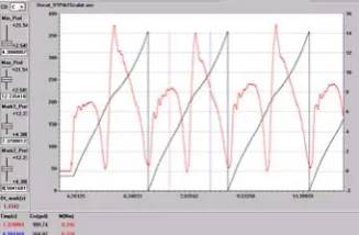
[image:5.595.317.537.54.225.2]We are interested the connection forces from cinematic joints. The Lagrange’s multipliers expressions, which we use in connection forces calculus, are much complex to present in this paper, and so we present a few connection forces laws.
[image:5.595.87.251.248.355.2]Fig.6. Variation law of ϕ1 angle and the M1 torque.
[image:5.595.312.547.303.478.2]Fig.7. Variation law in time of the
R
21x [N] reaction forceFig.8. Variation law in time of the
R
21y [N] reaction forceFig.10. Variation law in time of the
R
32y [N] reaction forceV. NUMERICAL PROCESSING FOR ELASTO-DYNAMIC ANALYSIS A. Planar connecting rod (4)
0,002004 0,002006 0,002008 0,00201 0,002012 0,002014 0,002016 0,002018 0,00202
0 0,5 1 1,5 2 2,5 3
time [sec]
d
isp
lac
em
en
ts [
m
m
]
Deplasari biela plana
Fig.11. Variation law in time of the resulted elastic displacement for the connecting rod in planar motion (4)
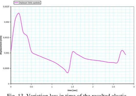
B. Spatial connecting rod (2)
0,00E+00 1,00E-07 2,00E-07 3,00E-07 4,00E-07 5,00E-07 6,00E-07 7,00E-07 8,00E-07
0 0,5 1 1,5 2 2,5 3
time [sec]
s
tra
in [
m
m
/mm
]
[image:5.595.66.268.387.531.2]Deformatii biela spatiala
[image:5.595.308.549.532.712.2] [image:5.595.68.267.564.709.2]0 0,0005 0,001 0,0015 0,002 0,0025
0 0,5 1 1,5 2 2,5 3
time [sec]
d
isp
la
cemen
t [
m
m]
[image:6.595.53.289.50.217.2]Deplasari biela spatiala
Fig. 13. Variation law in time of the resulted elastic displacement, by von Mises method
VI. CONCLUSION
We built mathematical models for dynamic analysis of mobile mechanical systems. These models were created by considering the elements as rigid ones in Newton-Euler formalism. This formalism was completed with Lagrange’s multipliers. In order to develop these mathematical models we go through the following steps:
- we develop the cinematic mechanism by identifying the analytical expressions for positions, speeds and accelerations of the mass centres;
- we identify the cinematic constrain equations (31); - we determine the (18x26) proper Jacobi for the equation system which governs the mechanism cinematic;
- we build the mass matrices (34) with 26x26 dimension; - we identify the generalized force vector (35);
- we define the generalized coordinate’s vector and we build the equation system which administrates the mechanism movement in dynamic regime.
The (36) equation system serves at dynamic inverse analysis, in order to determine the Lagrange’s multipliers vector with (38) relation. We elaborated a flexible program which follows the steps mentioned above, with a flexible structure. This structure permits to pass easily from the direct dynamic analysis to the inverse one. The dynamic inverse analysis’s aim was to determine the (11) correlations between connection forces components from the cinematic joints in dynamic regime.
At paragraph 2 we present a method for dynamic analysis of a multibody system in Newton – Euler formalism. In this case, the generalized coordinate’s vector has two important components. One of them define the position and orientation of the cinematic rigid element and the other define the elastic or flexible coordinates, respectively nodal coordinates. In motion equations interfere the following matrices:
M- mass matrix,K - stiffness matrix, Jq - Jacobi matrix,
λ - Lagrange’s multipliers vector, Qa - the vector of external generalized forces Qn - speeds quadratic vector which consists the gyroscopic components and Coriolis, obtained by differentiating the kinetic energy in rapport with time and the mechanism generalized coordinates. With this matrices we build the equations system no (17), which governed the movement of a mobile mechanical system with deformable elements.
The procedure presented in this paper is based on flexible matrix formalism, easily to implement on a computer, especially for the fact that the motion equation matrices are partitioned in rapport with a generalized coordinate’s character.
By computing the mathematical models, we obtain the variation laws in time for the cinematic joint’s connection forces. These are useless in finite element modeling of the wiper windshield mechanism’s dynamic response. The cinematic scheme was presented in fig. 5.
REFERENCES
[1] J. Aggirebeitia, R. Aviles, I. F. De Bustos, G. Ajuria, „A method for the study of position in highly redundant multibody systems in environments with obstacles,” IEEE transactions and robotics and
automation, vol.18, no.2, pp.257-263, 2002.
[2] J. Aggirebeitia, R. Aviles, I. F. De Bustos, G. Ajuria, „ Inverse position problem in highly redundant multibody systems in environments with obstacles”, Mechanisms & Machine Theory, vol. 38, pp. 1215-1235, 2003.
[3] R. Aviles, M.B. Ajuria, M.V. Hormaza, A. Herandez, „A procedure based on finite elements for the solution of nonlinear problems in the kinematic analysis of mechanisms”, Finite
Elements in Analyis and Design, vol.22, pp.304-328, 1996.
[4] J. Aggirebeitia, I. F. De Bustos, R. Aviles, „A Beam-type finite element modelling for velocity and acceleration analysis of 2D mechanisms”, 12th IFToMM Congress, Besancon, June 18-21, 2007.
[5] R. Aviles, G. Ajuria, E. Amezua, V. Gomez Garraz, “A finite element approach to the position problem in open loop variable geometry trusses”, Finite Elements in Analyis and Design, vol.34, pp.233-255, 2000.
[6] W. L. Cleghorn, „Analysis and design of high-speed flexible mechanism”, Phd. thesis, University of Toronto, 1980. [7] W. L. Cleghorn, R.G. Fenton, B. Tabarrok, “Steady-state
vibrational response of high-speed flexible mechanisms”,
Mechanism and Machine Theory, 19(4/5), 1984.
[8] N. Dumitru, A. Margine, M. Cherciu, A. Ungureanu, G. Catrina, “Organe de masini – arbori si lagare, proiectarea prin metode clasice si moderne”, Technical publishing house, 2008. [9] N. Dumitru, G. Nanu, “Mechanisms and mechanical
transmissions”, Universitaria Publishing house, 2007. [10] N. Dumitru, M. Cherchiu, A. Zuhair, “ Theoretical and
experimental modeling of the dynamic response of the mechanisms with deformable kinematics elements”, IFToMM
,Besancon, France, 2007.
[11] N. Dumitru, M. Cherchiu, A. Zuhair, “The finite element modeling of the dynamic response of the mechanisms”,
13thInternational Congres of Sound Vibration, Viena, Austria,
ISBN 3-9501554-5-7, 2006.
[12] N. Dumitru, A. Ungureanu, A. Margine, “ The general method for elastodynamical analysis of kinematic chains from the structure of walking robots”, IX International conference on the theory on
machines and mechanisms, pp.281-287 Liberec, Czech Republic,
2004.
[13] I. Fernandez-Bustos, J. Aggirebeitia, G. Ajuria, C. A. Angulo, “A new finite element to represent prismatic joint constraints in mechanisms”, Finite Elements in Analyis and Design, article in press.
[14] A. Hernandez, O. Altuzarra, R. Aviles, V. Petuya, “Kinematic Analysis of mechanism via a velocity equation on a geometric matrix”, Mechanisms & Machine Theory, vol.38, pp.1413-14295, 2003.
[15] D. Isobe, “A finite element scheme for calculating inverse dynamics of link mechanisms”, Fifth World Congress on