Generating distributed entanglement from electron currents

This content has been downloaded from IOPscience. Please scroll down to see the full text.

Download details:

IP Address: 138.251.14.57

This content was downloaded on 20/01/2014 at 09:54

Please note that terms and conditions apply.

Generating distributed entanglement from electron currents

View the table of contents for this issue, or go to the journal homepage for more 2011 New J. Phys. 13 103004

T h e o p e n – a c c e s s j o u r n a l f o r p h y s i c s

New Journal of Physics

Generating distributed entanglement from electron

currents

Yuting Ping1,5, Avinash Kolli2, John H Jefferson3 and Brendon W Lovett1,4,5

1_{Department of Materials, University of Oxford, Parks Road,}

Oxford OX1 3PH, UK

2_{Department of Physics and Astronomy, University College London,}

Gower Street, London WC1E 6BT, UK

3_{Department of Physics, Lancaster University, Lancaster LA1 4YB, UK} 4_{School of Engineering and Physical Sciences, Heriot-Watt University,}

Edinburgh EH14 4AS, UK

E-mail:[email protected]@hw.ac.uk

New Journal of Physics13(2011) 103004 (13pp)

Received 31 May 2011 Published 4 October 2011 Online athttp://www.njp.org/

doi:10.1088/1367-2630/13/10/103004

Abstract. Several recent experiments have demonstrated the viability of a

passive device that can generate spin-entangled currents in two separate leads. However, manipulation and measurement of individual flying qubits in a solid state system has yet to be achieved. This is particularly difficult when a macroscopic number of these indistinguishable qubits are present. In order to access such an entangled current resource, we therefore show how to use it to generate distributed, static entanglement. The spatial separation between the entangled static pair can be much higher than that achieved by only exploiting the tunnelling effects between quantum dots. Our device is completely passive, and requires only weak Coulomb interactions between static and flying spins. We show that the entanglement generated is robust to decoherence for large enough currents.

5_{Authors to whom any correspondence should be addressed.}

Contents

1. Introduction 2

2. Model and basic results 3

2.1. Attractor . . . 4

2.2. Convergence . . . 4

3. Generalisations 6

4. Decoherence 8

4.1. Static . . . 8

4.2. Flying . . . 10

5. Splitting efficiency 10

6. Other models 11

7. Conclusion 12

Acknowledgments 12

References 12

1. Introduction

Entanglement is an enabling resource for quantum computing (QC). It must be created and consumed in the process of executing any quantum algorithm [1], something which is most obviously apparent in the measurement-based model of QC [2,3]. In this picture, entanglement is first generated to build cluster states, before being consumed by single qubit measurements during the execution of an algorithm. The initial entanglement can be generated between distant qubit nodes [4–6], each of which can have its own, dedicated, measurement apparatus. Distributed entanglement would also enable secure communication over long distances [7, 8] and quantum teleportation [9].

Devices that generate entangled currents of pairs of electron spins propagating down different leads have been proposed in theoretical work [10–12], and recent experiments [13,14] have begun to demonstrate their feasibility [15–17]. However, it is not clear how such an entangled resource could be used for any of the applications discussed above, since the control and measurement of a single flying solid state qubit has yet to be demonstrated experimentally. Furthermore, the macroscopic nature of the currents makes this even more difficult, especially when there are times when spin pairs enter the same lead [13, 14]. In this paper, we will show that it is possible to convert such mobile entanglement to a static form in a completely passive way, in a very simple device—thus opening up the possibility of quantum information processors based on entangled currents. Notably, our scheme produces a static pair of entangled electron spins that can have a much higher degree of separation (see section 4.2) than more conventional protocols for entanglement generation for which the separation is limited by quantum tunnelling or similar local interactions [15–17].

At the centre of our device is a spin-entangled current generator that outputs entangled pairs of spins fi down two different leads i. Each spin encounters a further, static, spin si downstream of the generator and interacts with it, as shown in figure 1. The generator is based on earlier proposals of a passive device that produces pairs of spin-entangled electrons, with each pair maximally entangled in the singlet Bell state|S_if = √1

lead 1

lead 2

Current 1

Current 2 static electron 1

static electron 2

Spin interactions between flying & corresponding static electrons

flying electron 1

flying electron 2

Spin Entangled Currents Generator

Figure 1. Illustration of our entanglement generation device. Two currents,

composed of successive electron pairs that are maximally spin-entangled, emerge from a generator and pass down two leads. A static electron is situated downstream of the generator close to each lead, and the static pair is spatially well separated. The mobile spins in each lead interact with corresponding static spins as they pass. Note that the two flying spins of the same Bell pair are not required to, and will normally not, arrive at the sites of interaction with their corresponding static spins at the same time.

The nature of the static spins is not important, but one possibility is that a single electron is confined in each of the two quantum dots that are fixed close to the leads. Other suitable architectures include endohedral fullerenes in carbon nanotube peapods [18], carbon nanobud structures [19], and surface acoustic waves whose minima isolate single electrons [20].

2. Model and basic results

Let us start with an effective Hamiltonian coupling the flying and static spins of the following form:

Hi =

gi

2(σ si

x σ fi

x +σ si

y σ fi

y )=gi(σ₊siσ fi

− +σ si

−σ fi

+ ), (1)

where the σ_±=(σx±iσy)/2 are the usual Pauli operators. The gi are X Y exchange coupling strengths that depend on the separation of the two spins. Each gi is time dependent since one of the two interacting spins is mobile. The time evolution operator Ui(t) for a general state

|9i(t)i =Ui(t)|9i(0)iof the static-mobile pairi, is then

Ui(t)=exp[−iθi(t)(σ₊siσ fi

− +σ si

−σ fi

+ )], (2)

where θi(t)= Rt

0 gi(t0)dt0/¯h. θi(t)is constant when [0,t] is chosen so that gi(0)andgi(t)are negligible. In the basis|↑si↑fii,|↑si↓fii,|↓si↑fii,|↓si↓fii,

Ui = 

  

1 0 0 0

0 cosθi −i sinθi 0 0 ₋i sinθi cosθi 0

0 0 0 1



  

2.1. Attractor

We first consider the case whereθ1=θ2=θ and initially the static spins are in the state|↑s1↑s2i. The starting state of the two static and the first pair of flying spins is then √1

2(|↑s1↑f1i|↑s2↓f2i −

|↑s1↓f1i|↑s2↑f2i). Using the product of 2 unitary operators of the form of equation (3), we find that after interaction the state becomes cosθ|↑↑is|Sif −i sinθ|Sis|↑↑if. Since this first flying pair will no longer interact with the static spins nor with the following flying pairs, we can trace out this first flying pair to find the density matrix describing the static pair after the interaction: cos2θ|↑↑ish↑↑|+ sin2θ|SishS|.

In order to find the behaviour of our system for multiple passages of flying qubits, we require the following four maps which describe a single interaction event,U1,U2:

|↑↑ish↑↑| 7→cos2θ |↑↑ish↑↑|+ sin2θ |SishS|;

|↓↓ish↓↓| 7→cos2θ |↓↓ish↓↓|+ sin2θ |SishS|;

|S_ishS| 7→1₄sin22θ(|↑↑ish↑↑|+|↓↓ish↓↓|)+ sin4θ |T0ishT0|+ cos4θ |SishS|;

|T_0ishT_{0| 7→ |}T_0ishT_0|,

(4)

where_|T0i =√1₂(|↑↓i+|↓↑i), another maximally entangled Bell state. These maps imply that the state _|T0is is an attractor for this process, and by tracking the states of the static spins through multiple passages of the flying spins it is clear that the system will converge towards this maximally entangled attractor; we need not consider any further maps since other static spin states are never accessed. This fixed point is also consistent with spin-invariant scattering of the flying singlets from a static|T_0itriplet, as can be verified directly from the Schr¨odinger equation.

2.2. Convergence

We now calculate the probabilities of obtaining the |T_0is state after a number of flying spin passages. The reduced density operator for the static spins after n iterations is, by definition, ρ(n)

s =Pn·P, where P ≡(|↑↑ish↑↑|,|↓↓ish↓↓|,|SishS|,|T0ishT0|)T is the vector of projection operators for the base states and Pn≡(P↑↑(n), P↓↓(n),PS(n),PT0(n))

T _{is the}

corresponding vector of probabilities. Under the map, equation (4), P7→LP and hence

ρ(n) s 7→ρ(

n+1)

s =Pn·(LP)=(LTPn)·P, i.e.

Pn7→Pn+1=M0Pn (5)

where, by direct substitution,

M0≡LT=



    

cos2_{θ 0} 1 4sin

2_{2θ 0} 0 cos2_θ 1

4sin

2_{2θ 0} sin2θ sin2θ cos4θ ₀

0 0 sin4θ 1



    

.

n 10 n 50 n 100 n 500

0.1 0.2 0.3 0.4 0.5θ/π 0.2

0.4 0.6 0.8 1.0 PT0

5 10 15 20 25 30 n 10

4 0.2

0.4 0.6 0.8 1.0

PT0

× 0

5 10 15 20 25 30 n 10

6

0.2 0.4 0.6 0.8 1.0

PT0

×

0 5 10 15 20 25 30 n 10

8

0.2 0.4 0.6 0.8 1.0

P_T 0

× 0

θ = 0.1

θ = 0.03 θ = 0.01

(a) (b)

(c) (d)

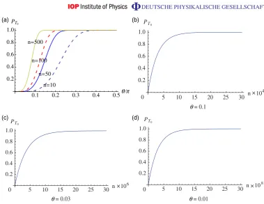
Figure 2. Plots of the probabilities of obtaining the |T_0ishT_0| state (a) against

θ

π, after 10,50,100,500 rounds of interactions, respectively; (b)–(d) against the number of rounds of interactions,n, forθ =0.1, 0.03 and 0.01, respectively.

equation (5), we have derived closed analytic expressions for Mn

0 and PT0(n). For the initial conditionsP0=(1,0,0,0)T, we have

1−PT0(n)=2

−4n−1

(Bn+Cn)₋5 + cos 2θ

A (B

n

−Cn)

, (6)

where

A₌p2 cos2θ(_{17 + cos 2}θ),

B₌7 + 8 cos 2θ+ cos 4θ−4Asin2θ, (7)

C₌7 + 8 cos 2θ+ cos 4θ+ 4Asin2θ.

For largen, when(4Asin2θ)/(7 + 8 cos 2θ+ cos 4θ)∈(0,2), i.e. whenθ .0.89,Cn_dominates over Bn_{and we have}

ln(1−PT0(n))'α(θ)n+β(θ) (8)

where α(θ)=ln(C/16)60 and β(θ)=ln[(A+ 5 + cos 2θ)/(2A)]. For θ1, (5 + cos 2θ)/

A_→1, and β(θ)→0. We plot the probability of obtaining the |T_0ishT_0| state against θ, for different values ofn in figure2(a).

¯ h

0 '67 ps, and therefore the time it takes for the static spins to converge to the|T0istate would be 20µs, 2 ms and 0.2 s forθ =0.1, 0.03 and 0.01, respectively. These time intervalst₀ are at least one order less in [13], and have the potential of being shortened further. Within the electron spin coherence time (>200µs) observed in [21], the convergence can occur for θ as small as 0.03 with the tunnelling rates achieved in [13]. We also point out that molecular systems have the potential for phase shiftsθ '1 due to larger exchange interactions arising from nanometre length scales; for example the exchange coupling in a nanotube/fullerene system may be several orders of magnitudes greater than in gated semiconductor devices [22].

3. Generalisations

Let us now generalize our analysis to include arbitrary coupling strengths (θ16=θ2) and arbitrary starting states for the static qubits. With the time evolution operators Ui defined as in equation (3), we can find a completely positive map Ls which represents the effect on the static spin density operatorρsof a passing flying qubit pair:

ρ(k+1)

s =Ls[ρs(k)]=Trf[(U1 O

U₂)(ρ_s(k)Oρ(_fk))(U₁OU₂)†], (9) where Trf denotes the partial trace [1] over the mobile spins, andρf = |SifhS|.

Equation (9) corresponds to a set of 16 recurrence relations for the elements of ρ_s(k). When θ1=θ2, four of these relations decouple from all the others, as we found in our argument earlier. The superoperator L_s is not a linear map, and we thus vectorize the density operator states by listing the entries in the following order as a column vector:

(ρ11ρ12. . . ρ14ρ21. . . ρ24ρ31. . . ρ44)T=:ρ˜. The map corresponding to the action of the superoperatorL_s,

˜

L_s:ρ˜(sk)7−→ ˜ρ( k+1)

s (10)

is then linear and can be written as a simple 16×16 matrix M, whose entries can be easily calculated using equation (9).

We find thatMalways has an eigenvalueλ=1, independent of the values of the coupling strengths. The multiplicity of this eigenstate is one, unless θ1 and θ2 are multiples of π. The corresponding eigenvector ρ_˜1 is then a single attractor state that is independent of the initial configuration of the static spins, which when transformed back to its density matrix form is

ρ1= 1 2(a+b)



   

a 0 0 0

0 b √1 2 0 0 √1

2 b 0

0 0 0 a



   

, (11)

where

a₌ (cosθ1−cosθ2)

2(_{1 + cos}θ

1cosθ2)csc3θ1csc3θ2

2√2 >0,

b₌ cscθ1cscθ2(csc

2_θ

1+ csc2θ2)−cotθ1cotθ2(2 + csc2θ1+ csc2θ2)

2√2 >

1

√

2. (12)

0.0 0.1

0.1 0.2

0.2 0.3

0.3 0.4

0.4 0.5

0.5

Θ2/Π

Θθ11//πΠ θ2/π

0.4

0.3

0.2

0.1

0.5 0.4 0.3 0.2 0.1 0.0

0.5

Θ2/Π

Θθ11//πΠ θ2/π

0.0 0.1 0.2 0.3 0.4 0.5 0.6 0.7 0.8 0.9 1.0

Fidelity EF

(a) (b)

Figure 3.Contour plots of (a) the fidelity between the attractorρ1and the|T0ihT0| state; and (b) the entanglement of formation EF of ρ1; each are plotted as a function ofθ1andθ2∈(0, π/2].

and their corresponding eigenvectors, when back in matrix form, all have trace zero and hence do not correspond to physical density operators. This has to be the case, as can be seen from the following argument. We can express any density state as ρ=P16i=1aiρi, since the set of eigenvectorsρ˜i (vectorized ρi) form a basis for M. The coefficients ai can take any values, so long as Tr(ρ)₌1 andρ is positive semi-definite and Hermitian. Hence, L_s[ρ]₌P16_i=1aiλiρi, or more generallyLn_s[ρ]=P16i=1aiλniρi, which also has trace 1 as a density matrix. Asn→ ∞,

λn

i →0∀|λi|<1 which is wheni =2,3, . . . ,16, and thusLn_s[ρ]→a1ρ1. So, Tr(Lns[ρ])→a1 since we defined Tr(ρ1)=1, and this requires a1=1. We thus obtain ρ=ρ1+6i16=2aiρi, and the trace requirement result in6_i16₌₂ai Tr(ρi)=0, which holds for various combinations ofai’s. This can only be true when Tr(ρi)=0∀i =2,3, . . . ,16..

Now, we can find how closeρ1 is to the|T0ihT0|state, for various values ofθ1 andθ2, by calculating the fidelity F as defined in [23]. In our case, we have

F(ρ₁,_|T_0ihT_0|)₌Tr( q_√

ρ1|T0ihT0|

√_ρ

1)= s

b+√1 2

2(a+b), (13)

which takes a value of unity whenθ1=θ2, as expected. Its contour plot in figure3(a) illustrates that even whenθ1andθ2 are different,ρ1 is still very close to the|T0ihT0|state for any(θ1, θ2) in the central region. The fidelity values also indicate the levels of degradation in our entangled resource through unequal coupling, the degree of which can be further established by calculating the Entanglement of Formation [24] E_F that the bipartite state ρ1 has [25]. We construct the contour plot for E_Fin figure3(b) showing that the degree of entanglementρ1possesses is very large, higher than 0.9, for any(θ1, θ2)in the central red region.

E_F

0.0 0.1 0.2 0.3 0.4 0.5 0

2 4 6 8 10 12 14

θ1/π

κ (θ1) in %

10 20 30 40 50 0.2

0.4 0.6 0.8 1.0

0 n 5 10 15 20 25 30

0.2 0.4 0.6 0.8 1.0 E_F

EF

n × 104

n × 104

25 26 27 28 29 30 0.9404

0.9412

0.9406 0.9408 0.9410

0

0.9400

(a) (b) (c)

Condition random θi∈(1.2, 1.4) random θi∈(0.1, 0.103)

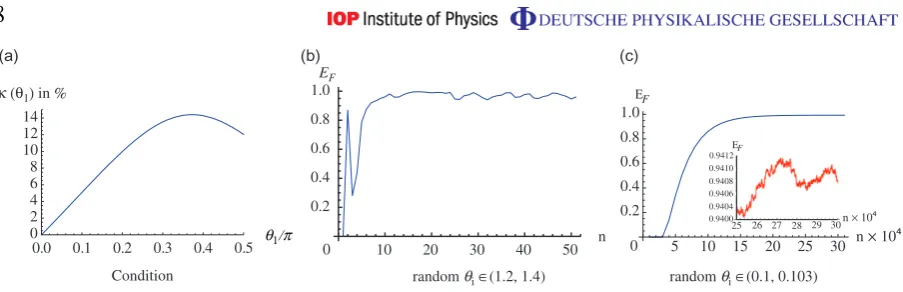
Figure 4.(a) Plot of the maximum allowed percentage difference κ(θ1)against

θ1/π for obtaining final EF(ρs)>0.9; (b,c) Example plots of the evolutions of E_F for the static spins as a function of the number of flying pairs n, for strong and weak random couplings, respectively. The inset in (c) zooms in on the corresponding fluctuations.

iteration k, as long as in each round1θ _{= |}θ1–θ2|satisfy the condition set in figure 3(b) such that (θ1, θ2) lies in the central red region. The maximum possible percentage difference in coupling strengths needed to maintain a highly entangled state may be defined as κ(θ1):= maxEF>0.9(1θ/θ1), and this quantity depends onθi itself, as shown in figure4(a). The maximum value forκ(θ1)occurs at aθ1 value away from π/2 because the maximum allowed1θ values for final E_F(ρ_s)>0.9 do not vary much forθi close toπ/2. Forθi as weak as 0.1, the maximum allowed percentage difference κ(0.1)'1.6%. We show two example plots for the evolutions of E_F for the static spins versusn forθi values that can vary within some range from round to round, in figures4(b) and (c). From these results we see that the convergence times are of the same order as for the case whenθ1=θ2 (see figure2) for both strong and weak couplings. We can also see that the condition on κ(θ1)in each round as specified in figure 4(a) only needs to be satisfied by the majority of the interaction rounds.

4. Decoherence

In practice, the environment interacts weakly with both static and flying spins, causing their decoherence. This will degrade our final entangled resource to some extent, and we shall consider such effects in this section.

4.1. Static

We first take into account the decoherence of the static spin pair, which in general will be coupled to the surrounding environment. The process can be modelled by a Markovian master equation [26] with decoherence channelskand corresponding decay ratesγk:

d

dtρs(t)=

15 X

k=1

γk(AkρsA†k− 1 2A

†

50 100 150 200 t ns 0.2

0.4 0.6 0.8 1.0

(a)

5 10 15 20I pA

0.75 0.80 0.85 0.90 0.95 1.00 Fidelity

(b)

E_F

Figure 5.Plots of the state of the static spin pair in the presence of pure dephasing

errors at randomθi ∈[1.3,1.4] and γ1=γ2=1 MHz: (a) fidelity of final states at equilibrium against current with the higher and lower lines representing the states right after and before X Y couplings, respectively; (b) E_Fagainst time for a spin-entangled current of 10 pA, with the dashed and solid lines representing the initial static spins being in the|T0iand the pure|↑↑istates, respectively. For the latter case, the initial rise and the subsequent fall inEFis due to the presence of the singlet state.

This assumption about the much shorter timescale also means that we do not need to consider decoherence during interactions events. Therefore, the evolution ofρs(t)can be tracked through application of the map L˜_s to describe interaction events and using the solution of the master equation between events. The resulting behaviour is a function of the productsγkt0, and we assumet₀to be constant for simplicity.

For certain decoherence models, analytical results can be found. For example, if we assume that there are two independent dephasing channelsσs1

z N

Is2 _{and I}s1Nσs2

z with ratesγ1andγ2 respectively, then forθ1=θ2the final fidelity of the state of the static spins with respect to|T0i is, immediately prior to an interaction events:

s

2 + 2e2(γ1+γ2)t0csc4θ−cot2θ(2 + 2 csc2θ)

4e2(γ1+γ2)t0csc2θ(2 csc2θ₋1)₋4 cot2θ(1 + 2 csc2θ). (15) We know that for the device to generate a large degree of static entanglement, we need

θ1 and θ2 to be in the central red region of figure 3. For example, working with random

θi ∈[1.3,1.4], calculations show that robustness to decoherence requires thatγkt0are at most on the order of 10−2_{. Forγ}

1=γ2=1 MHz (i.e. a coherence time of 1µs), figure5(a) illustrates the behaviour of the fidelity against current of flying pairs _te

(t_0∼1 ps) is needed forθi '0.03 (or at∼1 nA with spin coherence times in [21]). We see that decoherence will reduce the fidelity and hence the degree of entanglement of the steady state for the static spins, and thus in figure3the regions for high fidelity and high degree of entanglement will be narrower in the presence of decoherence.

4.2. Flying

Next, let us consider the decoherence of the flying singlets before they interact with the static spins. The whole analysis in section 3applies when we refine our model by allowing random error deviations(k)ofρ(_fk) from the singlet state in each round such that

ρ(k)

f =(1−( k)₎

|S_ifhS|+ 3 X

j=1

(k) j σ

f1

j |SifhS|σ f1

j , (16)

where the errors(k)

=P3j=1 (k)

j for eachkare due to spin-orbit coupling and interactions with the environment as the flying qubit propagates. Theσj’s are the Pauliσ1,2,3≡σx,y,zmatrices that correspond to different errors on one of the two flying qubits. We find that the single attractor state now has small error-dependent termscfor the corner entries on the minor diagonal ofρ1in equation (11), and bothaandbnow also depend on(_jk). As a result, the final E_F(ρ₁)is reduced, and the larger the errors the smaller it will be. We also find that the strong coupling regime can tolerate larger errors compared with weak coupling. This is because the static entanglement built up per round of interaction is much smaller for weak couplings and the errors(jk)can drastically reduce the accumulated entanglement. In either case, the average of (k) _{mainly determines the} final E_F for the static spins for fixed θi. For strong couplings, the error tolerance on (k) is of order 0.01, which corresponds to flying pairs with an average EF of ∼0.8–0.9. This results in a travelling distance on the millimetre scale for the flying spins at the Fermi velocity with typical coherence time of microseconds, before their interactions with the static pair. This error tolerance is much smaller for weak couplings, but this could also be feasible experimentally since couplings become weaker at high carrier speed, which also means a smaller interaction of the flying qubits with the environment before they arrive at the static qubit sites.

Therefore, for a given separation between the static spins, e.g. 1 mm (1µm, of conven-tional separations [15–17]), the time it takes the flying electrons (travelling at ∼105_{m s}−1₎ to arrive at the static qubit sites is 10 ns, much less than a typical spin coherence time (µs). Separations of centimetre scales can be achieved for longer spin coherence times [21].

5. Splitting efficiency

0.1 0.2 0.3 0.4 0.5 θ/π 0.2

0.4 0.6 0.8 1.0 EF

0 10 20 30 40 50n 0.0

0.2 0.4 0.6 0.8 1.0 E_F

20 40 60 80 100n 0.99980

0.99985 0.99990 0.99995 1.00000 E_F

(a) (b) (c)

ρ1s after one round of unsuccessful

splittings

(θ₁ ,θ₂) = (1.2, 1.3) & η = 95% (θ₁ ,θ₂) = (0.1, 0.1) & η = 99%

Figure 6. Plots for the evolutions of EF for the static spins: (a) of the attractor

stateρ1 after one round of interactions with the flying singlet pair entering the same lead, against variousθ_∈[0,π₂]; (b) and (c) examples of the corresponding steady states against number of roundsnwhen no other errors are present. Once the steady state is achieved, the success rates required could be lowered.

with E_F close to 1, as shown in figure6(b). In that case, the average E_F≈0.88 for η=95%. In the weak coupling regime, the steady state E_F of the static spins is large and fluctuates slightly for sufficiently high success rates, as shown in figure 6(c). The condition is that the amount of reduction in static entanglement by a single unsuccessful event should be smaller than the accumulated entanglement built up from a certain number N of consecutive successful splittings. In this case then η_{= N}N₊₁, and we find for example, when θ _'0.1, for η_'99.9%, then very high entanglement can be maintained (see figure6(c)).

In either case, for the current resource to be useful in terms of our scheme, the success rates for splittings should improve from those in [13,14] to at least 90%. Stronger currents will also make the scheme more robust to the various decoherence sources.

6. Other models

The above analysis was adapted to a Heisenberg exchange model by replacing the effective Hamiltonian in equation (1) with

H_i0₌ gi

2(σ si

x σ fi

x +σ si

y σ fi

y +σzsiσzfi). (17)

We then obtained similar results for the Heisenberg exchange model; the only difference is that this time the singlet state is the only attractor for equation (9), and the condition of similar coupling strengths is now replaced by the requirement of θ1(k)+θ2(k)'π in each round of interaction (see figure7in comparison with figure 3). Given this understanding, the results on the decoherence effects as well as the splitting efficiency are also similar.

0.2 1.0

0.8

0.6

0.4

0.2

0 0.4 0.6 0.8 1.0

θ2/π

θ1/π

θ2/π

θ1/π

1.0 1.0

0.8

0.8 0.6

0.6 0.4

0.4 0.2

0.2 0

0.0 0.1 0.2 0.3 0.4 0.5 0.6 0.7 0.8 0.9 1.0

Fidelity EF

(a) (b)

Figure 7. Contour plots for the single attractor state of the static spins in the

Heisenberg exchange model: (a) fidelity with respect to the singlet state as a function ofθi ∈[0, π]; (b) EFas a function ofθi ∈[0, π].

7. Conclusion

We have shown that distributed and static spin entanglement can be generated from a source of entangled current and weak, passive, Coulomb interactions. The entanglement generated is robust to various error sources. We therefore anticipate that spin entangled currents can be utilized in the way we have proposed in a wide range of experimental systems.

Acknowledgments

BWL acknowledges the Royal Society for a University Research Fellowship. YP thanks Hertford College, Oxford for a scholarship.

References

[1] Nielsen M A and Chuang I L 2000Quantum Computation and Quantum Information(Cambridge: Cambridge University Press)

[2] Raussendorf R and Briegel H J 2001 A one-way quantum computerPhys. Rev. Lett.865188

[3] Kok P and Lovett B W 2010 Introduction to Optical Quantum Information Processing (Cambridge: Cambridge University Press)

[4] Barrett S D and Kok P 2006 Efficient high-fidelity quantum computation using matter qubits and linear optics

Phys. Rev.A71060310

[6] Cabrillo C, Cirac J I, Garc´ıa-Fern´andez P and Zoller P 1999 Creation of entangled states of distant atoms by interferencePhys. Rev.A591025

[7] Lo H-K and Chau H F 1999 Unconditional security of quantum key distribution over arbitrarily long distances

Science2832050

[8] Shor P W and Preskill J 2000 Simple proof of security of the BB84 quantum key distribution protocolPhys. Rev. Lett.85441

[9] Bennett C H, Brassard G, Crepeau C, Josza R, Peres A and Wootters W K 1993 Teleporting an unknown quantum state via dual classical and Einstein–Podolsky–Rosen channelsPhys. Rev. Lett.701895

[10] Saraga D S and Loss D 2003 Spin-entangled currents created by a triple quantum dot Phys. Rev. Lett.

90166803

[11] Oliver W D, Yamaguchi F and Yamamoto Y 2002 Electron entanglement via a quantum dotPhys. Rev. Lett.

88037901

[12] Kolli A, Benjamin S C, Coello J G, Bose S and Lovett B W 2009 Large spin entangled current from a passive deviceNew. J. Phys.11013018

[13] Hofstetter L, Csonka S, Nygard J and Schoenenberger C 2009 Cooper pair splitter realized in a two-quantum-dot Y-junctionNature461960

[14] Herrmann L G, Portier F, Roche P, Yeyati A L, Kontos T and Strunk C 2010 Carbon nanotubes as Cooper-pair beam splittersPhys. Rev. Lett.104026801

[15] Recher P, Sukhorukov E V and Loss D 2001 Andreev tunneling, Coulomb blockade and resonant transport of nonlocal spin-entangled electronsPhys. Rev.B63165314

[16] Recher P and Loss D 2002 Superconductor coupled to two Luttinger liquids as an entangler for electron spins

Phys. Rev.B65165327

[17] Bena C, Vishveshwara S, Balents L and Fisher M P A 2002 Quantum entanglement in carbon nanotubes

Phys. Rev. Lett.89037901

[18] Watt A A R, Sambrook M R, Burlakov S V, Porfyrakis K and Briggs G A D 2008 Probing the interior environment of carbon nano-test-tubes arXiv:0810.3124v1

[19] Nasibulin A Get al2007 A novel hybrid carbon materialNature Nanotechnol.2156

[20] Barnes C H W, Shilton J M and Robinson A M 2000 Quantum computation using electrons trapped by surface acoustic wavesPhys. Rev.B628410

[21] Bluhm H, Foletti S, Neder I, Runder M, Mahalu D, Umansky V and Yacoby A 2010 Long coherence of electron spins coupled to a nuclear spin bath arXiv:1005.2995v1

[22] Ge L, Montanari B, Jefferson J H, Pettifor D G, Harrison N M and Briggs G A D 2008 Modeling spin interactions in carbon peapods using a hybrid density functional theoryPhys. Rev.B77235416

[23] Jozsa R 1994 Fidelity for mixed quantum statesJ. Mod. Opt.412315

[24] Wootters W K 1998 Entanglement of formation of an arbitrary state of two qubitsPhys. Rev. Lett.802245

[25] Munro W J, James D F V, White A G and Kwiat P G 2001 Maximizing the entanglement of two mixed qubits

Phys. Rev.A64030302

[26] Breuer H-P and Petruccione F 2002The Theory of Open Quantum Systems(Oxford: Oxford University Press) [27] De Jongh L J and Miedema A R 2001 Experiments on simple magnetic model systemsAdv. Phys.50947