Evaluating Neural Machine Translation in English Japanese Task

Evaluating Neural Machine Translation in English-Japanese Task

Zhongyuan Zhu Weblio Inc.

chugen.shu@weblio.co.jp

Abstract

In this paper, we evaluate Neural Machine Translation (NMT) models in English-Japanese translation task. Various network architectures with dif-ferent recurrent units are tested. Addi-tionally, we examine the effect of us-ing pre-reordered data for the train-ing. Our experiments show that even simple NMT models can produce bet-ter translations compared with all SMT baselines. For NMT models, recovering unknown words is another key to ob-taining good translations. We describe a simple workaround to find miss-ing translations with a back-off sys-tem. To our surprise, performing pre-reordering on the training data hurts the model performance. Finally, we provide a qualitative analysis demon-strates a specific error pattern in NMT translations which omits some informa-tion and thus fail to preserve the com-plete meaning.

1 Introduction

In the last two decades, Statistical Machine Translation (SMT) with log-linear models in the core has shown promising results in the field. However, as stated in (Duh and Kirch-hoff, 2008), log-linear models may suffer from the underfitting problem and thus give poor performance. While for recurrent neural net-works (RNNs), as demonstrated in (Mikolov et al., 2010), they brought significant improve-ment in Natural Language Processing tasks. In their research, RNNs are shown to be capa-ble of giving more prediction power compared with conventional language models when large training data is given. Using these neural

lan-guage models to rescore SMT outputs gener-ally gives better translation results (Auli and Gao, 2014). Other approaches rescore with RNNs that predict the next word by taking the word in current step and _S as inputs (Kalch-brenner and Blunsom, 2013; Cho, Merrien-boer, et al., 2014). Here, _S is a vector rep-resentation summarizes the whole input sen-tence.

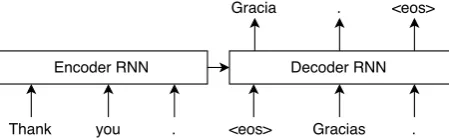
Neural machine translation is a brand-new approach that samples translation results di-rectly from RNNs. Most published models in-volve an encoder and a decoder in the net-work architecture (Sutskever, Vinyals, and Le, 2014), called Encoder-Decoder approach. Fig-ure 1 gives a general overview of this approach. In Figure 1, the vector output_Sof the encoder RNN represents the whole input sentence. Hence, S contains all information required to produce the translation. In order to boost up the performance, (Sutskever, Vinyals, and Le, 2014) used stacked Long Short-Term Memory (LSTM) units for both encoder and decoder, their ensembled models outperformed phrase-based SMT baseline in English-French trans-lation task.

Figure 1: Basic neural network architecture in Encoder-Decoder approach

Recently, by scaling up neural network mod-els and incorporating some techniques during the training, the performance of NMT models have already achieved the state-of-the-art in English-French translation task (Luong et al.,

61

2015) and English-German translation task (Jean et al., 2015).

In this paper, we describe our works on ap-plying NMT to English-Japanese translation task. The main contributions of this work are detailed as follows:

• We examined the effect of using different network architecture and recurrent units for English-Japanese translation

• We empirically evaluated NMT models trained on pre-reordered data

• We demonstrate a simple solution to re-cover unknown words in the translation results with a back-off system

• We provide a qualitative analysis on the translation results of NMT models

2 Recurrent neural networks

Recurrent neural network is the solution for modeling temporal data with neural networks. The framework of widely used modern RNN is introduced by Elman (Elman, 1990), it is also known as Elman Network or Simple Recurrent Network. At each time step, RNN updates its internal stateht based on a new input xt and

the previous state ht₋1, produces an output

yt. Generally, they are computed recursively

by applying following operations:

ht=f(Wixt+Whht−1+bh) (1)

yt=f(Woht+bo) (2)

Where f is an element-wise non-linearity, such as sigmoid or tanh. Figures 2 illustrates the computational graph of a RNN. Solid lines in the figure mark out the Affine transfor-mations followed with a non-linear activation. Dashed lines indicate that the result of previ-ous computation is just a parameter of next operation. The bias termb_h is omitted in the illustration.

RNN can be trained with Backpropagation Through Time (BPTT), which is a gradient-based technique that unfolds the network through time so as to compute the actual gra-dients of parameters in each time step.

Figure 2: An illustration of the computational graph of a RNN

2.1 Long short-term memory

For RNN, as the internal statehtis completely

changed in each time step, BPTT algorithm dilutes error information after each step of computation. Hence, RNN suffers from the problem that it is difficult to capture long-term dependencies.

Long short-term memory units (Hochre-iter and Schmidhuber, 1997) incorporate some gates to control the information flow. In ad-dition to the hidden units in RNN, memory cells are used to store long-term information, which is updated linearly. Empirically, LSTM can preserve information for arbitrarily long periods of time.

Figure 3 gives an illustration of the compu-tational graph of a basic LSTM unit. In which, input gate it, forget gate ft and output gate

ot are marked with rhombuses. “×” and “+”

are wise multiplication and element-wise addition respectively. The computational steps follows (Graves, 2013), 11 weight pa-rameters are involved in this model, compared with only 2 weight parameters in RNN. We can see from Figure 3 that the memory cells ct can keep unchanged whenft outputs 1 and

it outputs 0.

2.2 Gated recurrent unit

Gated recurrent unit (GRU) is originally pro-posed in (Cho, Merrienboer, et al., 2014). Similarly to LSTM unit, GRU also has gating units to control the information flow. While LSTM unit has a separate memory cell, GRU unit only maintains one kind of internal states, thus reduces computational complexity. The computational graph of a GRU unit is demon-strated in Figure 4. As shown in the figure, 6 weight parameters are involved.

Figure 4: An illustration of a GRU unit

3 Network architectures of Neural Machine Translation

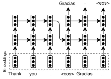
A basic architecture of NMT is called Encoder-Decoder approach (Sutskever, Vinyals, and Le, 2014), which encodes the input sequence into a vector representation, then unrolls it to generate the output sequence. Then softmax function is applied to the output layer in or-der to compute cross-entropy. Instead of using one-hot embeddings for the tokens in the vo-cabulary, trainable word embeddings are used. As a pre-processing step, “<eos>” token is appended to the end of each sequence. When translating, the token with the highest proba-bility in the output layer is sampled and input back to the neural network to get next output. This is done recursively until “<eos>” is ob-served. Figure 5 gives a detailed illustration of this architecture when using stacked multi-layer recurrent units.

3.1 Soft-attention models in NMT

As stated in (Cho, Merriënboer, et al., 2014), two critical drawbacks exist in the basic Encoder-Decoder approach: (1) the perfor-mance degrades when the input sentence gets longer, (2) the vocabulary size in the target

Figure 5: Illustration of a basic neural network architecture for NMT with stacked multi-layer recurrent units.

size is limited.

Attentional models are first proposed in the field of computer vision, which allows the re-current network to focus on a small portion in the image at each step. The internal state is updated only depends on this glimpse. Soft-attention first evaluates the weights for all pos-sible positions to attend, then make a weighted summarization of all hidden states in the en-coder. The summarized vector is finally used to update the internal state of the decoder. Contrary to hard-attention mechanism which selects only one location at each step and thus has to be trained with reinforce learning tech-niques, soft-attention mechanism makes the computational graph differentiable and thus able to be trained with standard backpropa-gation.

The application of soft-attention mechanism in machine translation is firstly described in (Bahdanau, Cho, and Bengio, 2014), which is referred as “RNNsearch” in this paper. The computational graph of a soft-attention NMT model is illustrated in Figure 6. In which, the encoder is replaced by a bi-directional RNN, the hidden states of two RNNs is finally con-catenated in each input position. At each time step of decoding, an alignment weight

ai is computed based on the previous state of the decoder and the concatenated hidden state of position i in the encoder. The align-ment weights are finally normalized by soft-max function. The weighted summarization of the hidden states in the encoder is then fed into the decoder. Hence, the internal state of the decoder is updated based on 3 inputs: the previous state, weighted summarization of the encoder and the target-side input token.

The empirical results in (Bahdanau, Cho, and Bengio, 2014) show that the performance of RNNsearch does not degrade severely like normal Encoder-Decoder approach.

4 Solutions of unknown words

A critical practical problem of NMT is the fixed vocabulary size in the output layer. As the output layer uses dense connections, en-larging it will significantly increase the com-putational complexity and thus slow down the training.

According to existing publications, two kinds of approaches are used to tackle this problem: model-specific and translation-specific approach. Well known model-specific approaches are noise-contrastive train-ing (Mnih and Kavukcuoglu, 2013) and class-based models (Mikolov et al., 2010). In (Jean et al., 2015), another model-specific solution is proposed by using only a small set of tar-get vocabulary at each update. By using a very large target vocabulary, they were able to outperform the state-of-the-art system in English-German translation task.

Solutions of Translation-specific approach usually take advantage of the alignment of to-kens in both sides. For examples, the proposed method in (Luong et al., 2015) annotates the unknown target words with “unkpos_i” instead of “unk”. Where the subscriptiis the position

of the aligned source word for the unknown target word. The alignments can be obtained by conventional aligners. The purpose of this processing step put some cues for recovering missing words into the output. By applying this approach, they were able to surpass the state-of-the-art SMT system in English-French translation task.

5 Experiments

5.1 Experiment setup

In our experiments, we are curious to see how NMT models work in English-Japanese trans-lation and how well the existing approaches for unknown words fit into this setting. As Japanese language drastically differs from En-glish in terms of word order and grammar structure. NMT models must capture the se-mantics of long-range dependencies in a sen-tence in order to translate it well.

We use Japanese-English Scientific Paper Abstract Corpus (ASPEC-JE) as training data and focus on evaluating the models for English-Japanese translation task. In order to make the training time-efficient, we pick 1.5M sentences according to similarity score then fil-ter out long sentences with more than 40 words in either English or Japanese side. This pro-cessing step gives 1.1M sentences for training. We randomly separate out 1,280 sentences as valid data.

As almost zero pre-knowledge of NMT ex-periments in English-Japanese translation can be found in publications, our purpose is to con-duct a thorough experiment so that we can evaluate and compare different model archi-tectures and recurrent units. However, the limitation of computational resource and time disallows us to massively test various models, training schemes, and hyper-parameters.

In our experiments, we evaluated four kinds of models as follow:

• LSTM Search: Soft-attention model with LSTM recurrent units

• pre-reordered LSTM Search: Same as LSTM Search, but the model is trained on pre-reordered corpus

• LSTM Encoder-Decoder: Basic Encoder-Decoder model with 4 stacked LSTM layers

Most of the details of these models are com-mon. The recurrent layers of all the models contain 1024 neurons each. The size of word embedding is 1000. We truncate the source-side and target-source-side vocabulary sizes to 80k and 40k respectively. For all models, we in-sert a dense layer contains 600 neurons imme-diately before the output layer. We basically use SGD with learning rate decay as optimiza-tion method, the batch size is 60 and initial learning rate is 1. The gradients are clipped to ensure L2 norm lower than 3. Although we sort the training data according to the input length, the order of batches is shuffled before training. For LSTM units, we set the bias of forget gate to 1 before training (Jozefowicz, Zaremba, and Sutskever, 2015). During the translation, we set beam size to 20, if no valid translation is obtained, then another trail with beam size of 1000 will be performed.

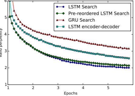
5.2 Evaluating models by perplexity For our in-house experiments, the evaluation of our models mainly relies on the perplexity measured on valid data, as a strong correla-tion between perplexity and translacorrela-tion per-formance is observed in many existing publi-cations (Luong et al., 2015). The changing perplexities of the models described in Section 5.1 are visualized in Figure 7.

1 2 3 4 5

Epochs 1

2 3 4 5 6

Valid perple

xity

LSTM Search

Pre-reordered LSTM Search GRU Search

LSTM encoder-decoder

Figure 7: Visualization of the training for dif-ferent models.

In Figure 7, we can see that soft-attention

models with LSTM unit constantly outper-forms the muti-layer Encoder-Decoder model. This matches our expectation as the alignment between English and Japanese is too compli-cated thus it is difficult for simple Encoder-Decoder models to capture it correctly. An-other observation is that the performance of the soft-attention model with GRU unit is sig-nificantly lower than that with LSTM unit. As this is conflict with the results reported in other publications (Jozefowicz, Zaremba, and Sutskever, 2015), one possible explanation is that some implementation issues exist and fur-ther investigation is required.

One surprising observation is that using pre-reordered data to train soft-attention models does not benefit the perplexity, but degrades the performance by a small margin. We show that the same conclusion can be drawn by measuring translation performance directly in latter sections.

5.3 Replacing unknown words

Initially, we adapt the solution described in (Luong et al., 2015), which annotate the un-known words with “unkpos_i”, where i is the position of aligned source word. We find this require source-side and target-side sentences roughly aligned. When testing on the soft-attention model with pre-reordered training data, we found this method can correctly point out the rough aligned position of a missing word. This allows us to recover the missing output words with a dictionary or SMT sys-tems.

However, for the training data in natural order, the position of aligned words in two languages differs drastically. The solution de-scribed above can hardly be applied as it an-notates the unknown words with relative po-sitions.

Figure 8: Illustration of replacing unknown words with a back-off system.

recovering the unknown words with a back-off system. We translate the input sentence using both a NMT system and a baseline SMT sys-tem. Assume the translation results are simi-lar, then if we observe an unknown word in the result of the NMT system, then it is reason-able to infer that the rarest word in the base-line result which is missing in the NMT result should be this unknown translation. This is demonstrated in Figure 8, the rarest word in the baseline result is picked out to replace the unknown word in the NMT result. Practically, the assumption will not be true, the results of NMT systems and conventional SMT sys-tems differ tremendously. Hence, some incor-rect word replacements are introduced. This method can be generalized to recover multiple unknown words by selecting the rarest word in a near position.

5.4 Evaluating translation performance

In this section, we describe our submitted sys-tems and report the evaluation results in the English-Japanese translation task of The 2nd Workshop on Asian Translation 1 (Nakazawa et al., 2015). We train these models with AdaDelta for 5 epochs. Then, we fine-tune the model with AdaGrad using an enlarged train-ing data, that each sentence contains no more than 50 words. With this fine-tuning step, we are able to achieve perplexity of 1.76 in valid data.

The automatic evaluation results are shown in Table 1. Three SMT baselines are picked for comparison. In the middle of the table, we list two single soft-attention NMT models with LSTM unit. The results show that train-ing models on pre-reordered corpus leads to degrading of translation performance, where the pre-reordering step is done using the model described in (Zhu, 2014).

Our submitted systems are basically an en-semble of two LSTM Search models trained on natural-order data, as shown in the bot-tom of Table 1. After we replaced unknown words with the technique described in 5.3, we gained 0.8 BLEU on test data. This is our first submitted system, marked with “S1”.

We also found it is useful to perform a

sys-1_{Our team ID is “WEBLIO MT”}

Table 1: Automatic evaluation results in WAT2015

Model BLEU RIBES PB basline 29.80 0.691 HPB baseline 32.56 0.746 T2S baseline 33.44 0.758 Single LSTM Search 32.19 0.797 Pre-reordered LSTM Search 30.97 0.779 Ensemble of 2 LSTM Search 33.38 0.800 + UNK replacing(S1) 34.19 0.802 + System combination 35.97 0.807 + 3 pre-reordered ensembles(S2) 36.21 0.809

tem combination based on perplexity scores. We evaluate the perplexity for all outputs pro-duced by a baseline system and the NMT model. These two sets of perplexity score are normalized by mean and standard devi-ation respectively. Then for each NMT result, we rescore it with the difference of perplexity against the baseline system. Intuitively, if the NMT result is better than the baseline result, the new score shall be a positive number. In our experiment, we pick the system described in (Zhu, 2014) as baseline system. We pick top-1000 results from NMT and the rest from the baseline system, this gives us a gain of 1.8 in BLEU.

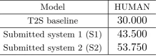
Table 2: Human evaluation results for submit-ted system in WAT2015

Model HUMAN T2S baseline 30.000 Submitted system 1 (S1) 43.500 Submitted system 2 (S2) 53.750

more normal LSTM Search models and put into the ensemble. We failed to do it because of insufficient time.

5.5 Qualitative analysis

To find some insights in the translation re-sults of NMT systems, we performed qualita-tive analysis on a proportion of held-out devel-opment data. During the inspection, we found many errors share the same pattern. It turns out that NMT model tends to make a perfect translation by omitting some information dur-ing the translation. In this case, the output tends to be a valid sentence, but the mean-ing is partially lost. One example of this phe-nomenon is shown in the following snippet:

Input: this paper discusses some systematic uncertainties including casimir force , false force due to electric force , and various factors for irregular

uncertainties due to patch field and detector noise .

NMT result: ここ で は ， Ｃａｓｉｍｉｒ 力 を

考慮 し た いく つ か の 系統 的 不 確実 性 に つ い て 論 じ た 。

Reference: Ｃａｓｉｍｉｒ 力 や 電気 力 に よ

る 偽 の 力 ， パッチ 場 や 検出 器 雑音 に よ る 不 規則 な 不確か さ の 種々 の 要因 を 含め ， 幾 つ か の 系統 的 不確か さ を 論 じ た 。

6 Conclusion

In this paper, we performed a systematic eval-uation of various kinds for NMT models in the setting of English-Japanese translation. Based on the empirical evaluation results, we found soft-attention NMT models can already make good translation results in English-Japanese translation task. Their performance surpasses all SMT baselines by a substantial margin ac-cording to RIBES scores. We also found that NMT models can work well without extra data processing steps such as pre-reordering. Fi-nally, we described a simple workaround to recover unknown words with a back-off sys-tem.

However, a sophisticated solution for deal-ing with unknown words is still an open ques-tion in the English-Japanese setting. As some patterns of mistakes can be observed from the translation results, there exists some space for further improvements.

References

Auli, Michael and Jianfeng Gao (2014). “De-coder integration and expected bleu train-ing for recurrent neural network language models”. In: Proceedings of the 52nd An-nual Meeting of the Association for Com-putational Linguistics (ACL’14), pp. 136– 142.

Bahdanau, Dzmitry, Kyunghyun Cho, and Yoshua Bengio (2014). “Neural ma-chine translation by jointly learning to align and translate”. In: arXiv preprint arXiv:1409.0473.

Cho, Kyunghyun, Bart van Merrienboer, et al. (2014). “Learning Phrase Representa-tions using RNN Encoder–Decoder for Sta-tistical Machine Translation”. In: Proceed-ings of the 2014 Conference on Empiri-cal Methods in Natural Language Process-ing (EMNLP). Doha, Qatar: Association for Computational Linguistics, pp. 1724–1734. Cho, Kyunghyun, Bart van Merriënboer, et

al. (2014). “On the Properties of Neural Machine Translation: Encoder–Decoder Ap-proaches”. In:Syntax, Semantics and Struc-ture in Statistical Translation, p. 103. Duh, Kevin and Katrin Kirchhoff (2008).

“Be-yond log-linear models: boosted minimum error rate training for N-best Re-ranking”. In: Proceedings of the 46th Annual Meet-ing of the Association for Computational Linguistics on Human Language Technolo-gies: Short Papers. Association for Compu-tational Linguistics, pp. 37–40.

Elman, Jeffrey L (1990). “Finding structure in time”. In: Cognitive science 14.2, pp. 179– 211.

Graves, Alex (2013). “Generating sequences with recurrent neural networks”. In: arXiv preprint arXiv:1308.0850.

Hochreiter, Sepp and Jürgen Schmidhuber (1997). “Long short-term memory”. In:

Neural computation 9.8, pp. 1735–1780. Jean, Sébastien et al. (2015). “On Using Very

Pa-pers). Beijing, China: Association for Com-putational Linguistics, pp. 1–10.

Jozefowicz, Rafal, Wojciech Zaremba, and Ilya Sutskever (2015). “An Empirical Explo-ration of Recurrent Network Architectures”. In: Proceedings of the 32nd International Conference on Machine Learning (ICML-15), pp. 2342–2350.

Kalchbrenner, Nal and Phil Blunsom (2013). “Recurrent Continuous Translation Mod-els”. In: Proceedings of the 2013 Con-ference on Empirical Methods in Natural Language Processing. Seattle, Washington, USA: Association for Computational Lin-guistics, pp. 1700–1709.

Luong, Thang et al. (2015). “Addressing the Rare Word Problem in Neural Machine Translation”. In:Proceedings of the 53rd An-nual Meeting of the Association for Com-putational Linguistics and the 7th Interna-tional Joint Conference on Natural Lan-guage Processing (Volume 1: Long Papers). Beijing, China: Association for Computa-tional Linguistics, pp. 11–19.

Mikolov, Tomas et al. (2010). “Recurrent neu-ral network based language model.” In: IN-TERSPEECH 2010, 11th Annual Confer-ence of the International Speech Communi-cation Association, Makuhari, Chiba, Japan, September 26-30, 2010, pp. 1045–1048. Mnih, Andriy and Koray Kavukcuoglu (2013).

“Learning word embeddings efficiently with noise-contrastive estimation”. In: Advances in Neural Information Processing Systems 26. Ed. by C.J.C. Burges et al. Curran As-sociates, Inc., pp. 2265–2273.

Nakazawa, Toshiaki et al. (2015). “Overview of the 2nd Workshop on Asian Translation”. In: Proceedings of the 2nd Workshop on Asian Translation (WAT2015).

Sutskever, Ilya, Oriol Vinyals, and Quoc VV Le (2014). “Sequence to sequence learn-ing with neural networks”. In: Advances in neural information processing systems, pp. 3104–3112.