Analyzing and simulating the coherent control model

(1)

ANALYZING AND SIMULATING THE

COHERENT CONTROL MODEL

Luuk Lubbers and Sean Stellingwer

Supervisors: Prof. Dr. Jennifer Herek and Dr. Ir. Herman L. Oerhaus

(2)

Abstract

A theoretical description and a simulation model for a coherent control model was derived and was experimentally veried. First, a simplied version of the coherent control model, where no distinction is made between pendula lengths, masses and spring constants, was considered and the equations of motion for that particular system were derived. This theoretical description was then analyzed, after which it was expanded to include all relevant parameters in the system.

The theoretical description was then implemented in a simulation model and this simulation model was subjected to various tests to ensure that is was performing as expected. To that end, both the experimental set-up and the simulation model were driven with a continuous sinusoidal shaped drive signal, of which the driving frequencyω was iteratively increased from small to large

values and the response of both systems was measured and compared. After verifying that the response of the simulation model adequately predicted the output of the experimental set-up, the lengths of various pendula were changed and the predicted response from the simulation model was compared to the response of the experimental set-up.

In the nal part of the research, the link between CARS and the coherent control model was briey discussed. The theory behind using a drive pulse instead of a continuous sinusoidal shaped drive signal was explained and the simulation model was subsequently subjected to a drive pulse to analyze its re-sponse. Lastly, the drive pulse was altered in the phase spectrum and the output of the simulation model was compared to the unaltered drive pulse response.

(3)

Chapter 1

Introduction

1.1 Coherent anti-Stokes Raman spectroscopy

Coherent anti-Stokes Raman spectroscopy, also known as CARS, is a spec-troscopy method used to visualize specic bonds in a molecule. A narrow-band pulse1_{could theoretically be used to excite one particular bond in a molecule, the}

energy that is stored in that bond will quickly dissipate into other bonds in the same molecule, leading to a loss of detection signal. To reduce the loss of detec-tion signal, a method called coherent control is often used. It works by shaping the pulse that is originally used to excite one specic bond to now excite all bonds in the molecule in such as way that the vibrations will (de)constructively interfere so that only the bond of interest will remaing vibrating.

1.2 Description of the demonstration model

In order to make the concept of coherent control comprehensible, a demonstra-tion model - a system of ve coupled pendula driven by a motor - has been built previously. The pendulum model is schematically drawn in gure 1.1. The set-up consists of ve coset-upled pendula, each coset-upled to its neighbouring pendula if present and also to a central drive axle. This drive axle is controlled by a motor which can in turn be controlled by a computer. This way, the pendulum model can be driven using various drive pulses in order to demonstrate the eect of an unoptimized and an optimized pulse. Using motion sensors, the movement of each pendulum is sent back to the computer which can in turn process the data and make changes to the drive pulse, if necessary.

To illustrate how each pendulum is connected to the drive axle and to neigh-bouring pendula, a close-up of the schematic drawing has been made, see gure 1.2.

1_{This is a pulse with a selective range of frequencies}

(6)

CHAPTER 1. INTRODUCTION 5

Figure 1.1: Schematic overview of the coherent control model

(7)

CHAPTER 1. INTRODUCTION 6

If there were no springs to attach each of the pendula to the axle or to a neighbouring pendulum, the pendula would be able to swing freely, independent of the drive axle's motion. This is achieved by using ball bearings to connect each pendulum to the axle as indicated in the schematic close-up. This way, the pendula can only be indirectly driven by the drive axle through the axle-coupling springs and each pendulum will aect the motion of its neighbouring pendula through the pendulum-coupling springs.

1.3 Thesis outline

(8)

Chapter 2

Theoretical description of the

set-up

In this chapter, a theoretical model of the pendulum set-up will be derived. First, a simple version of the set-up will be used to build a simple simulation model. This model will be analyzed to verify that the output is as can be expected, after which the model will be expanded to include parameters such as damping and varying spring constants.

2.1 The basics, simple system, amplitude response

Now that a clear picture has been formed of the pendulum set-up, it can be theoretically described so that a simulation model can be built. It is wise to start with a simple model in order to be able to analyze the simulation step by step, and to make sure that it is performing as it should. For this, initially the lengths

lof the dierent pendula as well as their massesmand the spring constants of

each type of spring in the system are chosen to be the same. Damping will also not be considered initially.

As mentioned, each of the pendula will ultimately be indirectly driven by a motor. The motor will turn a drive axle which will have an angle ofγ relative

to the vertical. Through a coupling spring, with spring constant κ, that is

connected to the drive axle and the pendulum itself, a force will be exerted on the pendulum. That force will be nonzero when the angle between the drive axle and the pendulum, which is dened to beθn−γ, is nonzero, where θn is

the angle of the nth pendulum relative to the vertical.

Additionally, each pendulum is connected by pendulum-coupling springs, with spring constanteκ, to its neighbouring pendula. That way each pendulum

will aect and will be aected by its neighbouring pendula. However, because of the set-up, not all pendula have two neighbours, some only have one. See Figure 1.1 for a schematic drawing, illustrating this.

(9)

CHAPTER 2. THEORETICAL DESCRIPTION OF THE SET-UP 8

The kinetic energyT1and the potential energyU1of pendulum 1, which has

only one neighbour, is given by

T1= 1 2m( ˙θ1l)

2₌1

2ml

2_θ˙2

1

U1 = mgy+ 1

2κ(θ1−γ)

2₊1

2κ˜(θ1−θ2) 2

= −mglcos(θ1) + 1

2κ(θ1−γ)

2₊1

2κ˜(θ1−θ2) 2

Whereg is the gravitational acceleration and y is the vertical position of the

mass1_.

For pendula that have two neighbouring pendula (namely pendula 2 through 4) the kinetic and potential energies are given by

Tn=

1 2m( ˙θnl)

2₌1

2ml

2_θ_˙2

n

Un = mgy+

1

2κ(θn−γ)

2₊1

2κ˜(θn−θn−1)

2₊1

2κ˜(θn−θn+1) 2

= −mglcos(θn) +

1

2κ(θn−γ)

2₊1

2κ˜(θn−θn−1)

2₊1

2κ˜(θn−θn+1) 2

wheren∈ {2,3,4}.

Finally, for pendulum 5, which like pendulum 1 only has one neighbouring pendulum, the kinetic and potential energies are given by

T5= 1 2m( ˙θ5l)

2₌1

2ml

2_θ˙2

5

U5 = mgy+1

2κ(θ5−γ)

2₊1

2κ˜(θ5−θ4) 2

= −mglcos(θ5) +1

2κ(θ5−γ)

2₊1

2κ˜(θ5−θ4) 2

Going one step further, the Lagrangians Ln≡Tn−Un forn∈ {1,2,3,4,5}

are then given by

L1 = 1 2ml

2_θ˙2

1+mglcos(θ1)− 1

2κ(θ1−γ)

2₋1

2κ˜(θ1−θ2) 2

L2 = 1 2ml

2_θ˙2

2+mglcos(θ2)− 1

2κ(θ2−γ)

2₋1

2κ˜(θ2−θ1)

2₋1

2κ˜(θ2−θ3) 2

L3 = 1 2ml

2_θ˙2

3+mglcos(θ3)− 1

2κ(θ3−γ)

2₋1

2κ˜(θ3−θ2)

2₋1

2κ˜(θ3−θ4) 2

L4 = 1 2ml

2_θ˙2

4+mglcos(θ4)− 1

2κ(θ4−γ)

2₋1

2κ˜(θ4−θ3)

2₋1

2κ˜(θ4−θ5) 2

L5 = 1 2ml

2_θ˙2

5+mglcos(θ5)− 1

2κ(θ5−γ)

2₋1

2κ˜(θ5−θ4) 2

(10)

CHAPTER 2. THEORETICAL DESCRIPTION OF THE SET-UP 9

The equations of motions for this system now follow from Lagrange's equa-tion2_,

∂ ∂t

_∂L

∂θ˙n

− ∂L

∂θn

= 0

Carrying out the dierentiation for each Langrangian gives a set of ve coupled non-linear second order dierential equations

¨

θ1+g_lsin(θ1) +a(θ1−γ) +b(θ1−θ2) = 0 ¨

θ2+glsin(θ2) +a(θ2−γ) +b(θ2−θ1) +b(θ2−θ3) = 0 ¨

θ3+g_lsin(θ3) +a(θ3−γ) +b(θ3−θ2) +b(θ3−θ4) = 0 ¨

θ4+g_lsin(θ4) +a(θ4−γ) +b(θ4−θ3) +b(θ4−θ5) = 0 ¨

θ5+g_lsin(θ5) +a(θ5−γ) +b(θ5−θ4) = 0

           (2.1) where

a≡ κ

ml2; b≡

e

κ ml2

The next step now is to take a trial solution and substitute it in (2.1). The motion of each pendulum is expected to be oscillatory, so a solution of the following form will be attempted

θn= Θneiωt

Where ω is the driving frequency and Θn can be complex.3 These trial

solutions are complex functions that are being used for their great eciency. Only the real part of each solution is physically signicant, so after the nal step of the solution, the real parts ofθn should be taken, if one is interested in

the time dependent solution.

In (2.1), a small angle approximation will be made, resulting insin(θn)≈θn.

Also, it is assumed that the driving motion can be described by γ = γ0eiωt,

whereγ0is a real number.4

Substituting the trial solutions into (2.1) and canceling the common expo-nential factor yields

−ω2Θ1+g_lΘ1+a(Θ1−γ0) +b(Θ1−Θ2) = 0

−ω2_Θ

2+g_lΘ2+a(Θ2−γ0) +b(Θ2−Θ1) +b(Θ2−Θ3) = 0

−ω2_Θ

3+g_lΘ3+a(Θ3−γ0) +b(Θ3−Θ2) +b(Θ3−Θ4) = 0

−ω2_Θ

4+g_lΘ4+a(Θ4−γ0) +b(Θ4−Θ3) +b(Θ4−Θ5) = 0

−ω2_Θ

5+g_lΘ5+a(Θ5−γ0) +b(Θ5−Θ4) = 0

           (2.2)

2_{This is Lagrange's equation when dissipative forces are not considered. Those forces will} be considered in section 2.3.

3_{A complex amplitude has a magnitude and a phase, which are the two arbitrary constants} necessary in the solution of a second-order dierential equation. Thus, the trial solution can be equally written asθn=|Θn|ei(ωt−φn). When there is no damping, the pendula will either carry a zero orπphase with respect to a sinusoidal driving signal. As a result the amplitude will always be real. Therefore, the complex amplitude is especially useful when a damped system is being considered, because the solution in this case might carry any phase.

(11)

CHAPTER 2. THEORETICAL DESCRIPTION OF THE SET-UP 10

This constitutes a set of coupled second order linear dierential equations, which allows the introduction of the transformation matrixM. Collecting terms

with a common factorΘn yields

M       Θ1 Θ2 Θ3 Θ4 Θ5      

=aγ0

      1 1 1 1 1       (2.3) where M≡      

β −b 0 0 0

−b β+b −b 0 0

0 −b β+b −b 0 0 0 −b β+b −b

0 0 0 −b β

      and

β≡ −ω2+g

l +a+b

In order to nd the amplitude (and phase) response, (2.3) has to be solved forΘn. Using Cramer's rule [?], the solution is given by

Θn =

det(Mn)

det(M)

whereMn is the matrix formed by replacing the the n-th column of M by the vectoraγ0[1 1 1 1 1]T.

As the simple system (i.e. equal l, κ,˜κ, and m and without damping) is

being considered, an exact solution can be found. This exact solution has been obtained and is found to be

Θn =

aγ0

−ω2₊g l +a

(2.4)

2.2 Analyzing the result

The next step in further expanding this theoretical model is to analyze the result so far, to ensure that this derivation is correct and to understand the behaviour that this model describes.

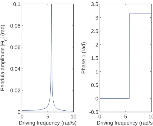
To start, from (2.4), the amplitude |Θn| and the phase response can be

plotted against the driving frequencyω. The result of this plot can be found in

(12)

CHAPTER 2. THEORETICAL DESCRIPTION OF THE SET-UP 11

0 5 10

0 0.02 0.04 0.06 0.08 0.1

Driving frequency (rad/s)

Pendula amplitude |

Θ n

| (rad)

0 5 10

-0.5 0 0.5 1 1.5 2 2.5 3 3.5

Driving frequency (rad/s)

Phase

φ

(rad)

Figure 2.1: Left: Pendula amplitude versus driving frequencyγ0with equal

pen-dulum lengths and no damping. Right: Pendula phase versus driving frequency

γ0 with equal pendulum lengths and no damping.

This is a somewhat surprising result, as (2.4) is independent of nand b as

can also be seen in the amplitude and phase response. Thus it can be concluded that in this case all pendula have the same amplitude response, all have a zero phase shift with respect to each other and they act as if there is no coupling between them. It would appear to be that no matter what the driving frequency is, not all of ve expected eigenmodes - that are to be expected since this system has ve pendula - can be excited5_{. To better understand this behaviour and to}

verify that this result is in fact correct, the eigenmodes and eigenfrequencies of this system will now be derived.

2.2.1 Eigenmodes and eigenfrequencies

The eigenmodes and corresponding eigenfrequencies of the system can be found by considering the system without driving (i.e. setting γ0 to zero), because

eigenmodes are characteristics of the system, independent of the system being driven or not. It is expected then, when the system is driven at a certain eigenfrequency, that its corresponding eigenmode will be excited. However, this happens not to be the case.

(13)

CHAPTER 2. THEORETICAL DESCRIPTION OF THE SET-UP 12

The simple system being considered does not include damping, which changes the eigenfrequencies of the system. The degree of damping in an oscillating sys-tem is commonly described in terms of the quality factorQ of the system. If

the system's quality factor, Q, is large enough, the eigenfrequencies approach

those of an undamped oscillator, as will be shown in section 2.2.1.2. Therefore, the eigenmodes and eigenfrequencies of the undamped system will be derived in the following section, followed by a similar derivation for the damped system.

2.2.1.1 Eigenfrequencies and eigenmodes

Finding the eigenmodes of the system is subject to solving

M       Θ1 Θ2 Θ3 Θ4 Θ5       =       0 0 0 0 0       (2.5)

Equation (2.5) has non-trivial solutions if and only ifdet(M) = 0. The

charac-teristic equation represented by this determinant is an equation of degree n in

ω2 _{and its roots might be labelled} _ω2

r. Theωr are the eigenfrequencies of the

system and can be shown to be

ω1=±

r

(g+al) l ω2=±

s

2g+ 2al+ 3bl+√5bl 2l

ω3=±

s

2g+ 2al+ 3bl−√5bl 2l

ω4=±

s

2g+ 2al+ 5bl+√5bl 2l

ω5=±

s

2g+ 2al+ 5bl−√5bl 2l

(2.6)

Note that all of theωr are real, as should be the case without damping, or

else the total energy of the system would decrease monotonically with the time. As all of the roots are distinct, the system is non-degenerate - that is, every mode is distinguishable. The dierent eigenmodes follow from subsituting the squared radicals ω2

r in (2.5) and solving for the amplitude vector accordingly.

(14)

CHAPTER 2. THEORETICAL DESCRIPTION OF THE SET-UP 13

~ η1 =

      1 1 1 1 1       ~ η2=

      −1 1 2( √

5 + 1) 0

−1

2(

√

5 + 1) 1       ~ η3 =       −1 −1 2( √

5−1) 0 1

2(

√

5−1) 1       ~ η4=       1 −1 2( √

5 + 3)

√

5 + 1

−1

2(

√

5 + 3) 1       (2.7) ~ η5 =

      1 1 2( √

5−3)

−√5 + 1 1

2(

√

5−3) 1      

These eigenvectors constitute an orthogonal set as their inner product is zero, h~ηi|~ηji= 0 (i6=j), which is to be expected, sinceMis symmetric. The

princi-ple of superposition then applies to the set of linearized dierential equations. Thus, the general solution forθn must be written as a linear combination of the

solutions for each of the k = 5 (where k is the number of oscillators) values of r,

θn(t) = Θ+n,1e

iω1t_{+ Θ}−

n,1e

−iω1t_{+ Θ}+

n,2e

iω2t_{+ Θ}−

n,2e

−iω2t_{+ Θ}+

n,3e iω3t

+Θ−_n,₃e−iω3t_{+ Θ}+

n,4e

iω4t_{+ Θ}−

n,4e−

iω4t_{+ Θ}+

n,5e

iω5t_{+ Θ}−

n,5e− iω5t

=

k

X

r=1

Θ+n,reiωrt+ k

X

r=1

Θ−n,re−iωrt

=

k

X

r=1

Θ+_n,reiωrt_{+ Θ}−

n,re

−iωrt

Because it is only the real part ofθn(t)that is physically meaningful, the nal

solution is (see also section 2.1)

θn(t) =<

" _k X

r=1

Θ+_n,reiωrt_{+ Θ}−

n,re− iωrt

#

=

k

X

r=1

Θ+_n,rcos(ωrt) + Θ−n,rcos(ωrt)

(2.8) This set of solutions does still have 2k arbitrary constants for each equation

for θn, giving a total of 2k2 = 50 unknown arbitrary constants. However,

the relation between dierent Θn,r is given by the eigenvectors ~ηr. Let ~ηm,r

designate the mth component of the rth eigenvector. Then for a given r,

(15)

CHAPTER 2. THEORETICAL DESCRIPTION OF THE SET-UP 14

These relations reduce the number of arbitrary constants with a factor k, namely to2k= 10, just as expected, because there are 5 equations of motion that are

of second order. The values of these constants are completely specied by the initial conditions of the system.

Equation (2.8) is the homogenous solution. In case of driving with damping, this is then the transient solution and the steady state solution is given by the particular solution. A particular solution would again be of the form θn,p = neiωt.

2.2.1.2 Eects of damping

In section 2.3 it will be shown how the equations of motion will change when damping (µ) is being included. The results will already be used in this

sub-section, to elaborate on the eigenfrequencies and eigenmodes of the damped system. The transformation matrix slighty alters withiµw added to its

diago-nal elements

M0=



   

β+iµω −b · · · 0

−b β+b+iµω · · · 0

... ... ... ...

0 0 · · · β+iµω

     with

β≡ −ω2+g

l +a+b

In a similar way as in subsection 2.2.1.1, the complex eigenfrequencies follow from M' as

ω1= 1 2µi±

s

−1

4µ2l+al+ 2g

l

ω2= 1 2µi±

s

−1

2µ

2_l_{+ 2}_g_{+ 2}_al_{+ 3}_bl₊√₅_bl

2l

ω3= 1 2µi±

s

−1

2µ2l+ 2g+ 2al+ 3bl−

√

5bl 2l

ω4= 1 2µi±

s

−1

2µ

2_l_{+ 2}_g_{+ 2}_al_{+ 5}_bl₊√₅_bl

2l

ω5= 1 2µi±

s

−1

2µ2l+ 2g+ 2al+ 5bl−

√

5bl 2l

(2.9)

(16)

CHAPTER 2. THEORETICAL DESCRIPTION OF THE SET-UP 15

is included, thus the same set of eigenvectors given by (2.7) applies.

In case of damping, it is the real part of ωr which determines the angular

frequency of the oscillatory motion. The imaginary part ofωr produces terms

of the form e−=(ωr)t in the expression for _θ

n(t) and therefore determines the

rate at which energy is being dissipated from the system.

If the Q-factor of the system is high enough, this will yield a small value

forµ, such that µ2 _{will be negligible, resulting in unchanged eigenfrequencies}

compared to the undamped system. Experiments have been done on the pen-dulum, and they are discussed in Chapter 4. It will be shown in that Chapter, that theQ-factor for a single uncoupled pendulum will be around 28, which is

fairly high. Therefore, in general, damping cannot be neglected as it will inu-ence the behaviour of the system, but it does not have a profound eect on the eigenfrequencies of the system.

2.2.1.3 The eigenmode paradox

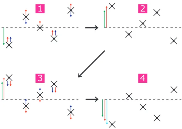
Dierent simulations were performed for the system being driven at one of the values ofωr. It became evident soon, that only one of the ve calculated

eigenmodes could be excited and maintained, for both the system with and without damping. This was eigenmode~η1, the mode in which every pendulum

has the same amplitude and phase. The reason for this happening can be explained by considering one of the other eigenmodes - say,~η2 - and observing

what happens when the system is being driven at the accompanying resonance frequencyω2. For simplicity, no coupling between pendula will be considered

intially, meaning thatb= 0. See Figure 2.2 for a schematic respresentation of

the maximum amplitudes of eigenmode~η2.

Figure 2.2: Schematic representation of eigenmode~η2. The dotted line indicates

zero amplitude.

(17)

CHAPTER 2. THEORETICAL DESCRIPTION OF THE SET-UP 16

1

2

4

3

Figure 2.3: Schematic representation of the forces on the dierent pendula in eigenmodeη2in the case of driving at dierent moments in the drive cycle.

in the case of driving.

In part 1 of this gure, the set-up is placed in the initial conditions of eigen-mode~η2. The green arrow next to the left-most pendulum graphically represents

the maximum amplitude of this particular pendulum. At exactly this moment, the drive axle is brought in motion. The red arrows indicate the direction in which the drive axle is then turning - this is arbitrarily chosen upward to begin with - and also indicate the force that is (indirectly) exerted on each pendu-lum by the drive axle. The blue arrows represent the direction in which each pendulum would move if undriven.

After half a period of the drive motion, the situation of the system will then be as presented in part 2 of the gure. The pendula that were below the dotted line in part 1 of the gure were pushed beyond their undriven maximum amplitude by the motion of the drive axle, whereas the pendula below the dotted line were slowed down and now have an amplitude that is less than their undriven maximum amplitude. To illustrate that the amplitude of the left-most pendulum has increased, a pink arrow was drawn alongside the original green arrow to indicate the new amplitude of that pendulum.

(18)

CHAPTER 2. THEORETICAL DESCRIPTION OF THE SET-UP 17

place for a long period of time. Again, the green and pink arrows together with a new blue arrow were added to illustrate that the amplitude of the left-most pendulum has increased after a full drive cycle.

The motion of this particular eigenmode will obviously die out as the pendula that initially move in-phase with the motor will be accelerated and the pendula that are π rad out of phase will be slowed down. In the case where there is

no coupling between pendula, the out-of-phase pendula will simply slow down, and then start to move in-phase with the motor, meaning that all pendula will eventually swing in-phase with each other. Since there is no coupling,b= 0and ω2=ω1- this follows from (2.6) - and the systems motion will explode6. In the

case where coupling between pendula is being considered, the motion is all but simple and beating will occur as the energy will be redistributed evenly across all pendula, meaning that after a transient period the pendula will eventually swing in-phase and all with the same nite amplitude - as in this caseω26=ω1

and the system will therefore not explode.

This conclusion can now be extended to each of the dierent eigenmodes of this system, yielding that in the driven case, none but eigenmode~η1 can be

excited when the system is being driven at the eigenfrequencies belonging to the respected eigenmodes, as was predicted by (2.4), ensuring that this model is in fact correct so far.

2.3 The extended system

In section 2.1, a theoretical model of the experimental set-up was derived which does not include damping, dierent lengths and masses of the pendula or dier-ent spring constants. In the experimdier-ental set-up, these parameters may dier signicantly, causing behaviour that the basic theoretical model cannot repro-duce. Since this model should accurately describe the behaviour of the ex-perimental set-up, all of these dierent parameters should be included in the theoretical model. In this section it will be described how this is done.

2.3.1 Damping

In Lagrangian mechanics, the Rayleigh dissipation function can be used to in-clude viscous forces and thus damping[3]. The denition of the Rayleigh dissi-pation function is given by

D= 1 2

e

m

X

j=1 e

m

X

k=1

µjkθ˙jθ˙k (2.10)

6_{In this ideal linear, uncoupled system, the relative phase between the drive signal and the} system is 0 rad forω < ω1and isπrad forω > ω1. The phase will be1₂πrad only at exactly

(19)

CHAPTER 2. THEORETICAL DESCRIPTION OF THE SET-UP 18

Whereme denotes the total amount of generalized coordinates in a system (in this

case ve),_θ˙

j andθ˙j denote the time derivatives of the generalized coordinates

andµjk are damping constants.

Equation (2.10) suggests that there are viscous forces that depend on the velocities of the dierent pendula and even on the relative velocities between pendula. In the experimental set-up, the coupling between neighbouring pen-dula is quite small when compared to the coupling between the penpen-dula and the driving axle - the spring constants of the pendulum-coupling springs are roughly ten times smaller. Therefore, it is assumed that the damping constantsµjk for j6=kare negligible and these terms can be ignored in the dissipation function.

Furthermore, it is assumed that damping due to air friction is signicantly larger than damping due to dissipation of heat in for example the axle-coupling springs or the ball bearings. This results inµjk=µfor each value ofj andk.

The aforementioned then implies that the dissipation function for this system is given by

D= 1 2µ( ˙θ

2

1+ ˙θ22+ ˙θ23+ ˙θ42+ ˙θ25) (2.11)

In the case of damping, Lagranges equation per pendulum is now given by

∂ ∂t

_∂L

∂θ˙n

− ∂L

∂θn

+ ∂D ∂θ˙n

= 0

Which, including (2.11), then yields

¨

θ1+g_lsin(θ1) +a(θ1−γ) +b(θ1−θ2) +µθ1˙ = 0 ¨

θ2+g_lsin(θ2) +a(θ2−γ) +b(θ2−θ1) +b(θ2−θ3) +µθ2˙ = 0 ¨

θ3+g_lsin(θ3) +a(θ3−γ) +b(θ3−θ2) +b(θ3−θ4) +µθ˙3 = 0 ¨

θ4+g_lsin(θ4) +a(θ4−γ) +b(θ4−θ3) +b(θ4−θ5) +µθ4˙ = 0 ¨

θ5+g_lsin(θ5) +a(θ5−γ) +b(θ5−θ4) +µθ5˙ = 0

Linearizing and lling in the same trial solution as before, this yields

−ω2Θ1+g_lΘ1+a(Θ1−γ0) +b(Θ1−Θ2) +iωµΘ1 = 0

−ω2Θ2+g_lΘ2+a(Θ2−γ0) +b(Θ2−Θ1) +b(Θ2−Θ3) +iωµΘ2 = 0

−ω2Θ3+g_lΘ3+a(Θ3−γ0) +b(Θ3−Θ2) +b(Θ3−Θ4) +iωµΘ3 = 0

−ω2_Θ

4+g_lΘ4+a(Θ4−γ0) +b(Θ4−Θ3) +b(Θ4−Θ5) +iωµΘ4 = 0

−ω2_Θ

5+g_lΘ5+a(Θ5−γ0) +b(Θ5−Θ4) +iωµΘ5 = 0

Which is the same as (2.2) when there is no damping (µ= 0).

2.3.2 Pendula lengths and masses

(20)

CHAPTER 2. THEORETICAL DESCRIPTION OF THE SET-UP 19

By assuming dierent lengths ln and dierent masses mn and deriving the

equations leading up to (2.2), this will yield

−ω2_Θ

1+_lg₁Θ1+a1(Θ1−γ0) +b1(Θ1−Θ2) +iωµΘ1 = 0

−ω2_Θ

2+_lg₂Θ2+a2(Θ2−γ0) +b2(Θ2−Θ1) +b2(Θ2−Θ3) +iωµΘ2 = 0

−ω2Θ3+_lg₃Θ3+a3(Θ3−γ0) +b3(Θ3−Θ2) +b3(Θ3−Θ4) +iωµΘ3 = 0

−ω2_Θ

4+_lg

4Θ4+a4(Θ4−γ0) +b4(Θ4−Θ3) +b4(Θ4−Θ5) +iωµΘ4 = 0

−ω2_Θ

5+_lg

5Θ5+a5(Θ5−γ0) +b5(Θ5−Θ4) +iωµΘ5 = 0

Where now

an ≡ κ mnl2n

; bn≡ e κ mnl2n

2.3.3 Spring constants

The nal contributing factor in the experimental set-up that will be considered is the variation between spring constants. In the experimental set-up they may vary by as much as 60 percent for the pendulum-coupling springs and by 30 percent for the axle-coupling springs - not exactly insignicant. Their addition to the theoretical description together with the previously added parameters now transform (2.2) to assume the following form

−ω2_Θ 1+_lg

1Θ1+a1(Θ1−γ0) +b1(Θ1−Θ2) +iωµΘ1 = 0

−ω2_Θ

2+_lg₂Θ2+a2(Θ2−γ0) +b2(Θ2−Θ1) +b3(Θ2−Θ3) +iωµΘ2 = 0

−ω2_Θ 3+_lg

3Θ3+a3(Θ3−γ0) +b4(Θ3−Θ2) +b5(Θ3−Θ4) +iωµΘ3 = 0

−ω2_Θ 4+_lg

4Θ4+a4(Θ4−γ0) +b6(Θ4−Θ3) +b7(Θ4−Θ5) +iωµΘ4 = 0

−ω2_Θ 5+_lg

5Θ5+a5(Θ5−γ0) +b8(Θ5−Θ4) +iωµΘ5 = 0              (2.12) Where now

an ≡ κn mnl2n

; b1≡ e κ1 m1l2

1

; b2≡ e κ1 m2l2

2

; b3≡ e κ2 m2l2

2

; b4≡ e κ2 m3l2

3

b5 ≡ eκ3

m3l2 3

; b6≡ eκ3

m4l2 4

; b7≡ eκ4

m4l2 4

; b8≡ eκ4

m5l2 5

(21)

Chapter 3

Constructing the simulation

model

In order to be able to predict the behaviour of the system, the next step is to make a simulation model that can receive an arbitrary drive input signal and presents the response of the system, θn(t). Initially, a model was built in

Simulink for its easy implementation, but quickly thereafter it became apparent that Simulink was not the best choice for our needs as it required more steps to change variables and process the results than is necessary. Therefore, a more complete model was built in MATLAB using its built-in ODE45 functionality. This chapter will briey discuss how both the Simulink and MATLAB models were built.

3.1 Simulink

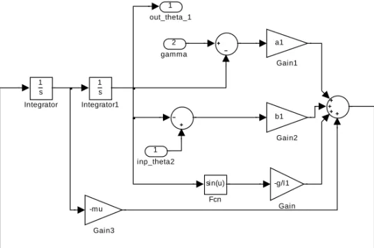
To build this model, (3.1) was taken and each of the equations was rewritten for _θ¨

n. Then, using integrators, θ˙n and θn could easily be calculated using

Simulink. For example, see Figure 3.1 for the Simulink subsystem of pendulum 1. The same procedure was followed for all other pendula and the subsystems were connected so that the complete system was now described in Simulink.

¨

θ1+_lg₁sin(θ1) +a1(θ1−γ) +b1(θ1−θ2) +µθ˙1 = 0

¨

θ2+_lg

2sin(θ2) +a2(θ2−γ) +b2(θ2−θ1) +b3(θ2−θ3) +µ

˙

θ2 = 0

¨

θ3+_lg

3sin(θ3) +a3(θ3−γ) +b4(θ3−θ2) +b5(θ3−θ4) +µ

˙

θ3 = 0

¨

θ4+_lg

4sin(θ4) +a4(θ4−γ) +b6(θ4−θ3) +b7(θ4−θ5) +µ

˙

θ4 = 0

¨

θ5+_lg

5sin(θ5) +a5(θ5−γ) +b8(θ5−θ4) +µ

˙

θ5 = 0



      

      

(3.1)

As an input for this Simulink model, initially a sine signal was added. This meant that ω and γ0 could be adjusted and the system could be run for a

predened amount of time. A graph was added which plottedθn as a function

of time.

(22)

CHAPTER 3. CONSTRUCTING THE SIMULATION MODEL 21

1

out_theta_1

1 s

Integrator1 1

s

Integrator

-mu

Gain3

b1

Gain2 a1

Gain1

-g/l1

Gain sin(u)

Fcn 2

gamma

1

inp_theta2

Figure 3.1: Simulink subsystem of pendulum 1

In the end, this model worked as expected and yielded proper results. For example, it could be observed that when all pendula had equal lengths, the amplitudes were all the same, no eigenmodes could be excited and at resonance frequency their amplitude grew enormously.

3.2 MATLAB

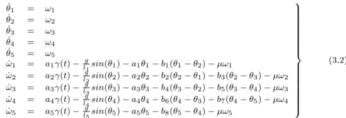
The set of dierential equations given by (2.12), can be numerically solved by MATLAB using the ODE45 function that integrates over time. Even though this function can only handle a set of rst order dierential equations, the set of second order dierential equations of can be solved by rewriting it as a system of rst order coupled dierential equations, see (3.2).

An advantage of solving it numerically, is that now every type of function forγ(t) might be imposed on the set of equations. A MATLAB le has been

programmed that solves these dierential equations subject to its boundary conditions, and plotsθn(t). See Appendix B for the accompanying MATLAB

(23)

CHAPTER 3. CONSTRUCTING THE SIMULATION MODEL 22

˙

θ1 = ω1

˙

θ2 = ω2

˙

θ3 = ω3

˙

θ4 = ω4

˙

θ5 = ω5

˙

ω1 = a1γ(t)−_lg

1sin(θ1)−a1θ1−b1(θ1−θ2)−µω1

˙

ω2 = a2γ(t)−_lg₂sin(θ2)−a2θ2−b2(θ2−θ1)−b3(θ2−θ3)−µω2

˙

ω3 = a3γ(t)−_lg

3sin(θ3)−a3θ3−b4(θ3−θ2)−b5(θ3−θ4)−µω3

˙

ω4 = a4γ(t)−_lg

4sin(θ4)−a4θ4−b6(θ4−θ3)−b7(θ4−θ5)−µω4

˙

ω5 = a5γ(t)−_lg₅sin(θ5)−a5θ5−b8(θ5−θ4)−µω5

                                   (3.2)

To illustrate the output of this model, an example output where the lengths, masses and spring constants are chosen the same is shown in Figure 3.2.

0 5 10

-0.5 0 0.5 time(s) | Θ 1 | (rad) pendulum 1

0 5 10

Figure 3.2: Output of the ODE45 model.

One important benet of this particular model is that it can be chosen to adopt the linear approximation or the non-linear approximation, if desired.

In Chapter 4 pulses will be dened that will drive the system. These pulses are computed discretely and are therefore only dened on certain time points, saytn, yieldingdt=tn+1−tn. When ODE45 is solving the dierential

equa-tions, it will calculate an optimal time step such that the spacing between suc-cessive time points will not be equal. Problem is then that the pulse is undened at the time points generated by ODE45, because they do not matchtn. To avoid

(24)

Chapter 4

Validating the simulation

model

A critical step in designing a simulation model is verifying its validity before predictions can be made using it. In order to verify the validity of the simulation model that was derived in the previous chapter, both the simulation model and the experimental set-up were exposed to an iterative test to (indirectly) measure the maximum amplitudes of the pendula as a function of varying driving frequencies. If these responses are - at least qualitatively - similar, this will demonstrate the validity of the simulation model.

In the end, to demonstrate that this model can now also be used to predict the behaviour of the experimental system, the lengths of some pendula will be altered and the simulation result will be compared to the experimental result.

4.1 The testing procedure

The goal is to drive the pendula with a continuous sinusoidal signalγ=γ0cos(ωt)

where ω is iteratively increased from small to large frequencies. The pendula

will initially all be at rest. In the simulation model and the experimental set-up the lengths of the dierent pendula will be chosen the same and are (for pen-dula 1 through 5)0.10m,0.15m,0.20m,0.25mand0.30mrespectively. After a

transitional period, the motion of the pendula will become stable, meaning the transient behaviour has died out and the maximum amplitude of each pendu-lum can be determined. In this case it is imperative that the driving amplitude

γ0 will be small enough to ensure linear motion. Even though in the end the

amplitudes will not quantitatively match1_{, the frequencies at which dierent}

pendula start to resonate should match. 1_{See section 4.1.2}

(25)

CHAPTER 4. VALIDATING THE SIMULATION MODEL 24

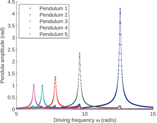
5 10 15

0 0.5 1 1.5 2 2.5 3 3.5 4 4.5

Driving frequency ω (rad/s)

Pendula amplitude (rad)

Pendulum 1 Pendulum 2 Pendulum 3 Pendulum 4 Pendulum 5

Figure 4.1: Maximum pendulum amplitude as a function of the driving fre-quency. The solid lines represent analytical data and the dotted lines indicate simulation data.

4.1.1 Simulation model

The simulation model was programmed to recieve the desired continuous sinu-soidal input as the drive signal. Linearity is assumed, so the driving amplitude can be arbitrarily chosen - here it was chosen to beγ0 = 0.1 rad. All other

parameters in the simulation model will be chosen as they were determined in [?]. As will be shown in section 4.1.3, the damping constant is determined to beµ= 0.1 and will be used here for a best approximation. The simulation was

driven for a suciently long time for the motion to become stable - roughly 150 seconds. In that case the maximum amplitude can safely be determined.

The result of this test can be seen in Figure 4.1. To illustrate that this result is correct, the previously determined analytical response from section 2.1 was added to the same graph.

It can be observed that both responses are in excellent agreement with each other. Because the drive input is a cosine, there is a nonzero amplitude at

ω= 0, and for all other frequencies the graphs match very well, meaning that

(26)

CHAPTER 4. VALIDATING THE SIMULATION MODEL 25

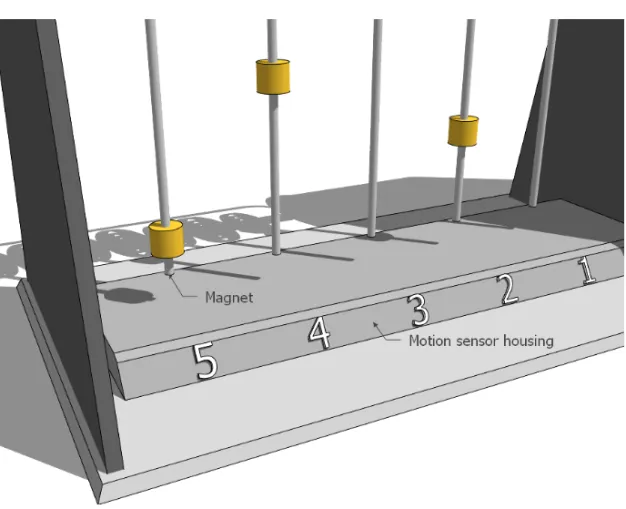
Figure 4.2: Close-up of the motion sensor housing and the magnets on the ends of the pendula

4.1.2 Experimental set-up

In the case of the experimental set-up, determining the maximum amplitude of a pendulum is not directly possible. Instead, the set-up features magnetic ux sensors in the motion sensor housing and small magnets attached to the end of each pendulum, see Figure 4.2. This way the magnetic ux as a function of time is measured, which can be interpreted as the velocity of the pendulum. If a large magnetic ux is measured, this will indicate that the pendulum was moving at a high velocity, which means that the pendulum in turn had a large amplitude. Therefore, if the pendula are driven for a suciently long time for the motion to become stable and the peak-to-peak voltage is determined during this stable period, it will be proportional to the maximum amplitude measured in the simulation model - only this time in volts.

Because the simulation model assumes linearity of the system, the driving amplitude is chosen to be as small as possible. As is visible in Figure 4.1, the pre-dicted maximum amplitude at resonance frequencies could exceedπrad, which

(27)

CHAPTER 4. VALIDATING THE SIMULATION MODEL 26

The experimental set-up was driven by a continuous sinusoidal signal for 160 periods of that particular signal. It was determined experimentally that the motion of the pendula was then fairly stable and the peak-to-peak voltage could safely be determined. After each measurement, the pendula were left to slow down, after which the frequency would be increased and another measurement could be performed. Since the simulation model predicts that the resonance frequencies lie between 5 and 15 rad/s, the experimental set-up was driven for frequencies in that same range.

The result of the measurement can be seen in Figure 4.3.

5 10 15

0 0.2 0.4 0.6 0.8 1 1.2 1.4 1.6 1.8

Pendula amplitude (Volts)

Figure 4.3: Result of experimental measurements.

The most obvious dierence between this result and the previously deter-mined analytical one is that the resonance frequencies for pendula which have short lengths lie far from the predicted frequencies but that the resonance fre-quencies for the pendula with longer lengths match fairly well. Since the lengths of the pendula inuence the position of the resonance frequencies greatly, ad-ditional testing was performed to determine the lengths of the pendula more accurately.

To do this, each pendulum was disconnected from all springs, ensuring it could swing freely. It was then left to swing for a certain period and the amount of full-period swings in this period was counted. From this, the period of swingT

could be determined and using the well known equation for the period of swing,

(28)

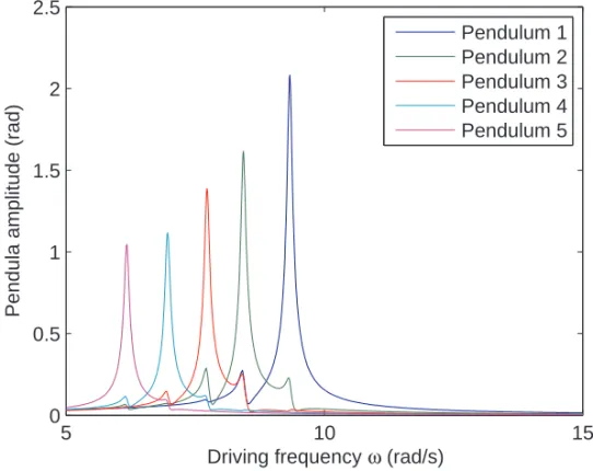
CHAPTER 4. VALIDATING THE SIMULATION MODEL 27

m,l3≈0.205 m,l4≈0.248m andl5≈0.311m. Using these corrected lengths

in the model results in a much better prediction of the resonance frequencies. See Figure 4.4.

5 10 15

0 0.5 1 1.5 2 2.5

Figure 4.4: Pendulum amplitudes versus driving frequency ω with adjusted

pendulum lengths using the simulation model

Another dierence between the simulation and the experimental measure-ments is that the resonance peaks are nonsymmetric in the case of the ex-perimental set-up. Approaching from the left, the amplitude per pendulum increases quite abruptly as the resonance frequency of that particular pendu-lum is reached, whereas to the right of the resonance frequency the pendupendu-lum maintains a relatively large amplitude, even for frequencies far from the reso-nance frequency. This nonsymmetry is very typical of nonlinear behaviour. To illustrate this further, simulations were performed where in one case linearity was assumed and in the other it was not. See Figure 4.5 for the result.

(29)

CHAPTER 4. VALIDATING THE SIMULATION MODEL 28

5 10 15

0 0.5 1 1.5 2 2.5 3 3.5 4 4.5

Figure 4.5: Pendula amplitudes versus driving frequency for linear and non-linear assumptions. The solid lines represent non-non-linear assumptions and the dashed lines represent linear assumption.

T = 2π

s

l g(1 +

1 16θ

2

0+

11 3072θ

4 0+· · ·)

Even though this equation does not hold exactly in the case of a coupled pendu-lum, it might be expected that the dependence onθ0will also be present in the

coupled case. This equation then implies that as the maximum amplitude of a non-linear pendulum increases, the amplitude response appears to shift to the left in the frequency domain2_{. The amount of shift is a function of higher order}

terms ofθ0. This means that asθ0increases more and more, so does the shift to

the left in the frequency domain of the amplitude response. Eventually, the shift will be so great that the resonance frequency, originally atωr is now shifted to

the left to a particular value ofω. The pendulum will therefore resonate, but at

a frequency lower than the resonance frequency expected from the linear model! As the pendulum still has a largeθ0, but after resonating will decrease again - in

the linear amplitude response it has "gone over the top" - the shift will decrease, meaning that the amplitude response shift becomes less. But here's the catch:

θ0decreases so it might be expected that the response might be similar to what

2_{This follows from the fact that the resonance frequency of a pendulum is given by}_ω₀₌

(30)

CHAPTER 4. VALIDATING THE SIMULATION MODEL 29

was seen approaching from the left in the frequency domain - a quick increase at rst, so now a quick decrease. However, sinceθ0 decreases, the shift to the

left of the amplitude response will also decrease, meaning that the maximum amplitude will decrease less quickly. The shift will then slowly decrease until at higher frequencies θ0 becomes small enough so that the shift is virtually zero

again and matches the linear approximation.

Another dierence between both results is that in the theoretical case the peak amplitudes increase as ω is increased, whereas in the experimental

mea-surements it can be observed that they in fact decrease as ω is increased. As

the frequency in the driving software was increased, it was observed that the maximum amplitude of the drive axle actually decreased. Of course, the ampli-tude should remain the same if a proper comparison is to be made between the theoretical and experimental set-up. When the driving amplitudeγ0decreases,

so will the maximum amplitude of a pendulum. Apparently, asω increases,γ0

decreases faster than the maximum amplitudes of the pendula would increase, if γ0 remained constant as function of frequency. This then results in a net

decrease of the maximum amplitudes of the pendula as ω increases, as was

observed.

The fact that the maximum amplitudes of the pendula in the theoretical case increase is due to the fact that for constantγ0, the torque exerted on the

pendula by the drive axle,τ, remains constant for allω. From ∂_∂t2θ2 =

τ ml2, it

then follows that shorther pendula have a larger angular acceleration, meaning that their maximum amplitudes will be larger.

The last major dierence between both results is that there appears to be a stronger coupling force between pendula, especially for pendula with shorter lengths. In testing the simulation model, it was found that altering the values of the coupling constants of the pendulum-couplinig springs by a relatively small amount aects the response of the system greatly. It could be that due to the self-made nature of the springs that although their properties were as measured at rst, over time their response has changed, causing this behaviour.

4.1.3 Estimation of the damping constant

As was discussed in section 4.1.1, most of the parameters in the system have al-ready been determined in previous reports or can easily be measured - all except for the damping constantµ. In this section, an value forµ will be determined

for completeness, where the experimental results found in the previous section will be used for the determination.

To begin, in section 2.2.1.2, the quality factor was already briey mentioned. TheQ-factor for a single resonator is given by [3]

Q≡ mωresonance

µ

(31)

CHAPTER 4. VALIDATING THE SIMULATION MODEL 30

eigenfrequency is given by

ω0=

r

g l +a

Subsituting this yields

µ= m

pg l +a

Q (4.1)

All parameters in (4.1) are known, except for Q. Since the system has been

observed to be underdamped, it is expected that the system is a high-Qsystem.

Therefore, the following equation for determiningQmay be used Q= ω0

∆ω

where∆ωis the width of the amplitude curve at half of its maximum amplitude.

Since this system is coupled, theQ-factors of all ve pendula will be determined

and averaged to provide a rough estimate of theQ-factor of the entire system.

See Figure 4.6 for an example of howω0 and∆ωwas determined for pendulum

5.

5.5 6 6.5 7

0 0.5 1 1.5 2

Pendula amplitude (Volts)

←

→ ∆ω

ω₀→ Pendulum 1_{Pendulum 2} Pendulum 3 Pendulum 4 Pendulum 5

Figure 4.6: ∆ω is dened as the width of the amplitude curve at half of its

maximum amplitude.

(32)

CHAPTER 4. VALIDATING THE SIMULATION MODEL 31

This is a useful estimation, as there exists no analytical formula for multiple coupled oscillators, that relatesQto the damping constant.

4.2 Adjusting the lengths

Now that the model has been analyzed and compared to the experimental set-up, it was found to behave as expected, so predictions can now be made using it. In this section, three dierent situations will be considered. For convenience, the system will now be considered linear, as then the analytical solution for the amplitudes of each pendulum can be used instead of using the simulation model3_.

4.2.1 Two pendula with equal lengths

For example, what happens when, instead of choosing the pendula to have the lengths as dened in section 4.1, two of those pendula say, pendula 1 and 5 -have the same length?

5 6 7 8 9 10

0 0.5 1 1.5 2

Pendula amplitudes (rad)

Figure 4.7: Pendula amplitude as a function of the driving frequency in the case that pendula 1 and 5 have identical lengths.

(33)

CHAPTER 4. VALIDATING THE SIMULATION MODEL 32

In the simulation model, this is easily altered. In this case the following lengths were changed: l1=l5= 0.311 m, and the other pendula lengths are as

previously dened. The result of this calculation is presented in Figure 4.7. As can clearly be observed, the model predicts that in this case pendula 1 and 5 will both have roughly the same resonance frequencies4 _{and they will}

also have roughly the same amplitudes. Both pendula 1 and 5 will have much larger maximum amplitudes if the driving frequency is chosen to be that of the resonance frequency of these pendula whereas the other pendula will have a relatively small amplitude. This situation was also tested in the experimental set-up and the exact same behaviour was observed, meaning the model ade-quately predicted this behaviour.

4.2.2 V-shape

Another interesting example is when the pendula lengths are chosen so that the system is symmetric in shape. Take for example a V-shape, where l1 = l5 = 0.155m,l2=l4= 0.183mandl3= 0.205m.

5 6 7 8 9 10 11 12

0 0.5 1 1.5 2

Figure 4.8: Pendula amplitude as a function of the driving frequency in the case of the lengths being chosen in a V shape.

(34)

CHAPTER 4. VALIDATING THE SIMULATION MODEL 33

the newly dened lengths, the expectation would be that there would only be three resonance frequencies. In the case where the actual real parameters are chosen, the result is as can be seen in Figure 4.8.

As can be seen, pendula 1 and 5 overlap very well, whereas pendula 2 and 4 overlap fairly well. This is obviously due to the non-ideal parameters of both pendula 2 and 4, but not unimportantly also of their neighbouring pendula as neighbouring pendula will greatly inuence each other. This behaviour was once again tested against the experimental set-up and the behaviour was as described by the model.

4.2.3 All pendula with equal lengths

The nal test will be where all pendula have the same length. As was derived in Chapter 1, in that case there should be only one resonance frequency of the system, and the amplitude responses as a function of the driving frequency should overlap - provided that all parameters are equal per pendulum. In the model, the lengths were chosen to be l1 =l2 =l3 =l4 =l5 = 0.205 m. The

response is as shown in Figure 4.9.

5 6 7 8 9 10 11 12

0 0.5 1 1.5 2

Figure 4.9: Pendula amplitude as a function of the driving frequency in the case of the lengths being chosen equal for all pendula.

(35)

CHAPTER 4. VALIDATING THE SIMULATION MODEL 34

no such thing will happen. To observe more closely what happens, a close-up is shown in Figure 4.10.

7.4 7.6 7.8 8 8.2

0 0.5 1 1.5 2

Figure 4.10: Close-up of the response in Figure 4.9.

(36)

Chapter 5

A driving pulse

In Chapter 2, a theoretical description of the set-up was made, where continuous driving was assumed of the formγ=γ0cos(ωt). In Chapter 4, the results of the

performed simulations were validated. It has been shown that the pendulum set-up has ve characteristic resonance frequencies, for ve dierent lengths of the pendula. By choosing one of these characteristic eigenfrequencies and driving the system at this specic frequency with a continuous sinusoidal signal, it was possible to excite one pendulum signicantly more than the others.

However, the pendulum set-up was built to explain and investigate the anal-ogy with CARS spectroscopy and coherent control. The point is that in CARS, molecules will always be excited with a certain broadband light pulse - they will be not be continuously excited. The reason for this is that the intensity of the received CARS signals scales with the cube of the intensity of the incoming signal, i.e. ICARS = χIIN3 , where χ is a proportionality factor. In general,

this constantχ is very small, such that the incoming signal has to have a high

intensity to be able to measure the CARS signal. A light pulse can have a much higher peak intensity than a continuous light beam while still outputtig the same amount of power. Using a pulse, then, is desirable, otherwise a laser with an output power in the order of MW would be required.

The problem is then translated back in terms of the pendulum model as nding a driving pulse that will excite one pendulum signicantly more than other pendula. In this Chapter, an attempt will be made to nd and dene such a pulse, where Chapters 2 and 4 will be used as guidelines.

5.1 General idea of the shaped pulse

From the CARS perspective, suppose that an incident pulse with a very narrow frequency spectrum, such that it has one specic frequency, strikes a molecule. This frequency can be chosen such that it matches the resonance frequency of one specic bond in a molecule, therefore exciting this specic bond. However, energy will immediately leak to other bonds due to coupling between adjacent

(37)

CHAPTER 5. A DRIVING PULSE 36

Figure 5.1: Exciting a molecule with a pulse [5].

atoms, resulting in them being indirectly excited as well. See Figure 5.1 for a schematic drawing.

The idea is then to take an incident pulse with a broader frequency spectrum, that contains the frequencies of all bonds in the molecule with the right ampli-tudes and phases for destructive interference, such that one specic bond will be excited signicantly more than others. See Figure 5.2 for another schematic drawing of this situation.

Figure 5.2: Exciting the same molecule, but now with a shaped pulse [5].

(38)

CHAPTER 5. A DRIVING PULSE 37

phase spectrum should look like. The next section will elaborate on this.

5.1.1 Flipping the phase of the driving signal

In Chapter 2, it was shown howΘn(ω)was derived. This formula is called the

frequency response or transfer function, because it describes how the system responds to dierent frequencies. When applying a driving signal γ(t), the

response of a pendulum in the frequency domain,_Θ˜_n₍_ω₎_{, is given by the product}

of the transfer function and the Fourier transform ofγ(t)

˜

Θn(ω) = Θn(ω)ˆγ(ω)

= |Θn(ω)|eiϕn(ω)|γˆ(ω)|eiϕd(ω) (5.1)

= |Θn(ω)||γ(ω)|ei(ϕn+ϕd)

Now suppose that γˆ(ω) has a frequency spectrum that is relatively wide

compared to the transfer functionsΘn(ω)and envelopes these transfer functions

at the same time, as shown in Figure 5.3. Because the fourier transform of a Gaussian is once again a Gaussian, this shape will be chosen for γˆ(ω) for

convenience. The larger the width of the Gaussian envelope, the more it will approach the Fourier Transform of a delta pulse, which is= {δ(t)}= 1. Thus,

if the width is chosen large enough, (5.1) simplies to

˜

Θn(ω)≈|Θn(ω)|ei(ϕn+ϕd) (5.2)

Equation (5.2) is an important result as it states that all of the frequency components that _Θ˜_n₍_ω₎ _{contains, might be given an identical phase. Setting}

the phase of the driving signalϕd opposite toϕn would do the job ϕd=−ϕn

The phase of a pendulumϕn changes as shown in Figure 5.3.

The phase of the driving signal should then be chosen equal to the light-blue dashed line. The polar plot in Figure 5.4 illustrates this idea: ifωincreases, the

blue circle will be traced in the direction of increasing numbers. Its correspond-ing phaseϕn, then runs from0 toπ. Now suppose the driving function traces

the green circle in the opposite direction as again indicated by the increasing numbers. Its corresponding phase ϕd then runs from 0 to −π. It is obvious

from (5.1), that their phases will add up to yield_Θ˜_n_{. The eect is then that}

the net response lies across the positive real axis, because all vectors will add up across these axis. Note that this would not be case when using a at phase,

ϕd = 0, as then horizontal vector components would cancel out, resulting in a

(39)

CHAPTER 5. A DRIVING PULSE 38

0 1 2 3 4

Pendula amplitude |

Θ n

| (rad)

← Gaussian envelope

0 5 ω

3 10 15

-4 -2 0 2 4

Pendula phase

φ n

(rad)

0 5 ω

3 10 15

Figure 5.3: The amplitude and phase response for a system of ve uncoupled pendula. The Gaussian envelope which is multiplied with in the frequency domain is shown as well. The blue dashed line represents the phase of this envelope, and has the opposite phase of pendulum 3.

-1.5 -1 -0.5 0 0.5 1 1.5

-1 -0.5 0 0.5 1

ℜ

ℑ

2 3 4 5 6

7

8

1

2

3

4 5 6 7 8

9

Pendulum transfer function Drive input function

(40)

CHAPTER 5. A DRIVING PULSE 39

ω₀

-π 0 π

Original driving phase Phase response pendulum Altered driving phase

2π

Figure 5.5: Changing the drivers phase by π at resonance frequency ω0, will

bring the driver and pendulum back in phase again.

In the remaining part of this Chapter, derivations will be made using the ideal phase response of the system for convenience, as the phase response does not dier too much from the ideal case as long as µ is not too large - which

it was previously determined not to be. Beside this, the driving axle of the pendulum model will probably not be able to follow the exact phase response due to its own resolution limitations.

In this ideal case, the phase jumps previously shown in Figure 5.3 will now assume the form of Figure 5.5. This phase jump is chosen to occur when the driving frequency equalsω0, the resonance frequency of the pendulum that is

to be excited. Only this pendulum will be aected by this phase ip, since all other pendula have amplitudes that are negligible at these frequencies, and a phase ip there will go unnoticed. The eect of this phase ip is similar to what was previously described for the non-linear case, although in this case, without the phase ip in the drive signal, the amplitude components of the pendulum would add up to a total of zero att= 0, whereas all amplitude components will

add up constructively if the phase ip is introduced. Therefore, this method should theoretically produce a much better response of the pendulum that is to be excited than before.

(41)

CHAPTER 5. A DRIVING PULSE 40

with a pulse with has the same shaped phase, cannot be expected to work as well in the uncoupled case, but still it is expected to work better than if no phase ip would be used.

0 5 10 15

-6 -5 -4 -3 -2 -1 0

Phase

φ

(rad)

Pendulum phases vs driving frequency with L = [0.1, 0.2, 0.3, 0.4, 0.5]

Figure 5.6: Phase behaviour of pendula in the coupled system, when using lineair approximation.

In section 5.1.2, the shape of the actual pulse will be determined when its phase spectrum is at, i.e. ϕ(ω) = 0, followed by a numerically inverse Fourier

transformed pulse in section 5.1.4, with the altered phase spectrum shown in Figure 5.5. These pulses will then be implemented as driving signals in the simulations, such that the behavior of both pulses can be investigated.

5.1.2 Dening the (angular) frequency spectrum of the

pulse

From Fourier analysis it is known that

Fne−ξt2(t)o=

r_π

ξe

−ω2

4ξ _ξ∈

(42)

CHAPTER 5. A DRIVING PULSE 41

(5.3) in frequency domain around+ν, settingξ= 1

2σ

2_{, multiplying by an}

arbi-trary constantαand adding a similar mirrored (inω= 0) Gaussian to preserve

symmetry, the new amplitude spectrum is then dened as

A(ω) =α

√

2π σ

e−(ω2+σν2)2 ₊_e− (ω−ν)2

2σ2

(5.4)

Note that the value of σ determines the width of the Gaussians, which has

to be chosen such that all of the system's eigenfrequencies are present in the amplitude spectrum, as explained in the previous section. Furthermore,ν will

be chosen equal to the resonance frequency of a pendula. The corresponding phase spectrum will only make sense when it is odd, because as was mentioned before, the time signal has to be real valued. It is initially dened as

ϕd(ω) = 0

Such that the frequncy spectrum of the time signal is dened as

ˆ

γ(ω) =A(ω)eiϕd(ω)

The signal in the time domain follows from the inverse Fourier transform

γ(t) = 1 2π

∞

ˆ

−∞

ˆ

γ(ω)eiωtdω

= αe−12σ 2_t2

(e−iνt+eiνt) = 2αe−12σ

2_t2

cos(νt) (5.5)

Apparently,γ(t)is a sinusoid with a Gaussian envelope. A plot of the

amplitude-and phase spectrum ofγ(t), as well as γ(t)itself with its Gaussian envelope is

shown in Figure 5.7. For convenience, the constants have been set toα= 1; σ= 1; ν= 5.

5.1.3 Using MATLAB for the inverse Fourier transform

In the previous subsection,γ(t)has been derived analytically. This becomes a

lot harder, if not impossible, when the phase spectrum will be changed. It was therefore decided to use the Inverse Fast Fourier Transform function of MAT-LAB, to transform the signal from frequency domain to time domain. Perform-ing an inverse Fourier transform usPerform-ing MATLAB on the amplitude and phase spectrum, shown in Figure 5.7, should yield the same result as the analytical re-sult of (5.5). However, they will not match in general. This is due to periodicity in the time domain assumed by the IFFT function, but the amplitude spectrum dened by (5.4) transforms intoγ(t), and is clearly non periodic. This problem

(43)

CHAPTER 5. A DRIVING PULSE 42

-5 0 5

-2 -1.5 -1 -0.5 0 0.5 1 1.5 2

γ

(t)

time (s)

-10 0 10

0 0.5 1 1.5 2 2.5 3

A(

ω

) and

φ

(

ω

)

ω

A(ω)

φ(ω)

Figure 5.7: On the left: amplitude and phase spectrum ofγ(t); On the right: γ(t)with the gaussian envelope.

interval from Te = [−100 100] is more than sucient, because both signals

could hardly be distinguished anymore. Eectively, MATLAB now sees a time signal which is apparently long enough to treat it as 'non-periodic'. Another consequence of MATLAB assuming periodicity is that the amplitude spectrum will scale with the length of the time interval, thusA(ω)∼1/Te.

When performing an inverse Fourier transform, it is imperative that the sam-pling frequencyωs is high enough, in order to be able to follow high frequency

components. The minimum sample rate required to completely reconstruct the time signal is the Nyquist frequencyωs= 2ωb, whereωbis the bandwidth of the

frequency spectrum. From (5.4) it follows that a sampling frequencyωsν+4σ

will be more than sucient. From the sample frequency, the corresponding time step then follows asdt= 2_ωπ

s.

The aforementioned describes the main issues and most important basics of the algoritm that carries out the inverse Fourier transform. See also Appendix B.

5.1.4 Re-dening the phase spectrum

The phase spectrum ofγ(t)will now be re-dened as explained in section 5.1,

(44)

CHAPTER 5. A DRIVING PULSE 43

can mathematically be represented in terms of the Heaviside functionH

ϕs(ω) =π[H(ω−ω0)− H(−ω−ω0)]

Changing the phase spectrum ofγ(t)will not change the energy content of the

phase altered signalγs(t), because their amplitude spectrum is the same

Ef =

1 2π

∞

ˆ

∞

|ˆγ(ω)|2dω= 1 2π

∞

ˆ

∞

A2(ω)dω= 1 2π

∞

ˆ

∞

|ˆγs(ω)| 2

dω

From this, one would conclude that the response of the system to the original pulse and phase altered pulse may be compared, since both signals put the same amount of energy into the system. However, a problem arises asγs(t)will not

converge to zero ast → ±∞ whereasγ(t) converges to zero quickly and is at

only one percent of its maximum when 1

2σ

2_t2_>₄_{. Obviously, one would want}

to drive the system with a pulse of a dened and nite duration. The dierence betweenγ(t)andγs(t)can be qualitatively understood in terms of the frequency

spectrum. A at phase spectrum, shown in Figure 5.7, results inγ(t)being built

up of cosines of dierent frequencies, centered aroundt= 0. Because they have

dierent frequencies, the cosines will go out of phase as |t| > 0, resulting in

destructive interference - hence the signal converges to zero for large |t|. If the at phase spectrum is now altered to the one shown in Figure 5.8, again cosines of dierent frequencies will add up. However, now not all of them will be centered aroundt= 0, therefore destroying the symmetry that γ(t)has. This

in turn then partially destroys the (complete) destructive interference and the signal will not converge to zero anymore.

To obtain a phase altered pulse with a nite duration, it was decided to cut oγs(t), which denes a new signalγs0(t). The typical cut o time, designated tc, has been made dependent on the typical width of the original pulse. The

typical width of the pulse has been dened as the time at which 1

2σ

2_t2 _{= 8}_,

to be on the safe side (the amplitude of the pulse will then be negligible, as it will be in the order of 10−4 _{radians), or} _t

typicalwidth = 4_σ. In general, this

value oftwill not be a root ofγs, and it would be better to avoidtc to be such

thatγs(tc)6= 0for practical reasons: the motor of the demo model always starts

with zero amplitude and dening a pulse which starts with a nite amplitude is therefore not feasible in practice. If one would just ignore this, the actual applied pulse would be slightly dierent.

An algorithm has been written that searches for the closest zero around

ttypicalwidth, see pendulum_inverse_fourier.m, added to Appendix B. This

newly found time value is then assigned tc. Note that because of symmetry,

once a root is known to be located at t = tc, another zero is automatically

located at −tc. Even though both pulses are now well dened on [−tc tc] ,

(45)

CHAPTER 5. A DRIVING PULSE 44

-4 -2 0 2 4 -2

-1.5 -1 -0.5 0 0.5 1 1.5 2

time (s)

γ

(t) and

γ s

(t)

Original pulse Phase altered pulse

-10 0 10

-4 -3 -2 -1 0 1 2 3 4

A(

ω

) and

φ

(

ω

)

Analyzing and simulating the coherent control model