http://wrap.warwick.ac.uk/
Original citation:Chaisemartin, Clément de and D'Haultfoeuille, Xavier (2015) Fuzzy differences-in-differences. Working Paper. Coventry: University of Warwick. Department of Economics. Warwick economics research papers series (WERPS) (1065). (Unpublished)
Permanent WRAP url:
http://wrap.warwick.ac.uk/73105
Copyright and reuse:
The Warwick Research Archive Portal (WRAP) makes this work of researchers of the University of Warwick available open access under the following conditions. Copyright © and all moral rights to the version of the paper presented here belong to the individual author(s) and/or other copyright owners. To the extent reasonable and practicable the material made available in WRAP has been checked for eligibility before being made available.
Copies of full items can be used for personal research or study, educational, or not-for-profit purposes without prior permission or charge. Provided that the authors, title and full bibliographic details are credited, a hyperlink and/or URL is given for the original metadata page and the content is not changed in any way.
A note on versions:
The version presented here is a working paper or pre-print that may be later published elsewhere. If a published version is known of, the above WRAP url will contain details on finding it.
Warwick Economics Research Paper Series
Fuzzy Differences-in-Differences
Clement de Chaisemartin and Xavier D'Haultfoeuille
October, 2015
Fuzzy Dierences-in-Dierences
∗Clément de Chaisemartin† Xavier D'Haultf÷uille‡
October 6, 2015
Abstract
In many applications of the dierences-in-dierences (DID) method, the treatment increases more in the treatment group, but some units are also treated in the control group. In such fuzzy designs, a popular estimator of treatment eects is the DID of the outcome divided by the DID of the treatment, or OLS and 2SLS regressions with time and group xed eects estimating weighted averages of this ratio across groups. We start by showing that when the treatment also increases in the control group, this ratio estimates a causal eect only if treatment eects are homogenous in the two groups. Even when the distribution of treatment is stable, it requires that the eect of time be the same on all counterfactual outcomes. As this assumption is not always applicable, we propose two alternative estimators. The rst estimator relies on a generalization of common trends assumptions to fuzzy designs, while the second extends the changes-in-changes estimator of Athey & Imbens (2006). When the distribution of treatment changes in the control group, treatment eects are partially identied. Finally, we prove that our estimators are asymptotically normal and use them to revisit applied papers using fuzzy designs.
Keywords: dierences-in-dierences, changes-in-changes, quantile treatment eects, partial identication, returns to education.
JEL Codes: C21, C23
∗This paper is a merged and revised version of de Chaisemartin & D'Haultf÷uille (2014) and de Chaise-martin (2013). We thank Yannick Guyonvarch for excellent research assistance, and are very grateful to Esther Duo and Erica Field for sharing their data with us. We also want to thank Alberto Abadie, Joshua Angrist, Stéphane Bonhomme, Marc Gurgand, Guido Imbens, Rafael Lalive, Thierry Magnac, Blaise Melly, Roland Rathelot, Bernard Salanié, Frank Vella, Fabian Waldinger, Yichong Zhang and participants at various conferences and seminars for their helpful comments.
1 Introduction
Dierence-in-dierences (DID) is a popular method to evaluate the eect of a treatment in the absence of experimental data. In its basic version, a control group is untreated at two dates, whereas a treatment group becomes treated at the second date. If the eect of time is the same in both groups, the so-called common trends assumption, one can measure the eect of the treatment by comparing the evolution of the outcome in both groups. DID can be used with panel or repeated cross-section data, when a policy is implemented at a given date in some groups but not in others. It can also be used when a policy aects individuals born after a given date. In such instances, birth cohort plays the role of time.
However, in many applications of the DID method, the treatment rate or intensity increases more in some groups than in others, but there is no group which experiences a sharp change in treatment, and there is also no group which remains fully untreated. In such fuzzy designs, a popular estimator of treatment eects is the DID of the outcome divided by the DID of the treatment, an estimator referred to as the Wald-DID. For instance, Duo (2001) uses a school construction program in Indonesia to measure returns to education. The author uses districts where many schools were constructed as a treatment group, and districts where few schools were constructed as a control group. Years of schooling for cohorts born after the program increased more in treatment districts. The author then estimates returns to schooling through a 2SLS regression in which dummies for cohorts beneting from the program and for being born in treatment districts are used as controls, while the instrument is the interaction of these two dummies. The coecient for treatment in this regression is the Wald-DID. A number of papers also estimate 2SLS regressions with time and group xed eects and with a function of time and group as the excluded instrument, or OLS regressions at the group×period level
with time and group xed eects. In our supplementary material, we show that the coecient of treatment in these two regressions is a weighted average of Wald-DIDs across groups. Such estimators have been frequently used by economic researchers. From 2010 to 2012, 10.1% of all papers published by the American Economic Review estimate either a simple Wald-DID, or the aforementioned IV or OLS regression. Excluding lab experiments and theory papers, this proportion raises to 19.7%.1 Still, to our knowledge no paper has studied whether these
estimators estimate a causal eect in models with heterogeneous treatment eects.
This papers makes the following contributions. We start by showing that the Wald-DID estimand is equal to a local average treatment eect (LATE) only if two strong assumptions are satised. First, time should have the same eect on all counterfactual outcomes, thus implying that the eect of the treatment should not vary over time. This assumption is often not applicable. For instance, in Duo (2001) it requires that the wage gap between high school graduates born in younger and older cohorts should be the same had they not completed high
school. If they had not completed high school, graduates of every cohort would have entered the labor market earlier, and would have had more labor market experience by the time their wages are observed. As returns to experience tend to be concave (see Mincer & Jovanovic, 1979), the wage gap between graduates born in younger and older cohorts would presumably have been lower if they had not completed high school. Second, when treatment increases both in the treatment and in the control group, treatment eects should be homogenous in the two groups. Indeed, in such instances the Wald-DID is equal to a weighted dierence between the LATE of treatment and control group units switching treatment over time. This weighted dierence can be interpreted as a causal eect only if these two LATEs are equal. The weights received by each LATE can be estimated. In Duo (2001), years of education increased substantially both in treatment and in control districts, so the Wald-DID in this paper is equal to a weighted dierence between returns to schooling in treatment and control districts, and returns in the control group receive a large negative weight. This weighted dierence estimates a causal eect only if returns to schooling are equal in the two groups of districts. This might be violated as control districts are more developed and could therefore have dierent returns. The IV and OLS regressions we study in our supplementary material suer from the same problem. They both estimate a weighted sum of LATEs, with potentially many negative weights as we illustrate by estimating these weights in two applications. Second, we propose two alternative estimators for the same LATE when the distribution of treatment is stable over time in the control group. Our rst estimator, which we refer to as the time-corrected Wald ratio (Wald-TC), is a natural generalization of DID to fuzzy designs. It relies only on common trends assumptions between the treatment and the control group, within subgroups of units sharing the same treatment at the rst date. Our second estimator, which we refer to as the changes-in-changes Wald ratio (Wald-CIC), generalizes the changes-in-changes estimator introduced by Athey & Imbens (2006) to fuzzy designs. It relies on the assumption that a control and a treatment unit with the same outcome and the same treatment at the rst period will also have the same outcome at the second period.2 Hereafter,
we refer to this condition as the common changes assumption. Our Wald-TC and Wald-CIC estimators both have advantages and drawbacks, which we discuss later in the paper.
Third, we show that under the same common trends and common changes assumptions as those underlying the Wald-TC and Wald-CIC estimands, the same LATE can be bounded when the distribution of treatment changes over time in the control group. The smaller this change, the tighter the bounds. Fourth, we show how these results extend to settings with many group and periods, and how one can incorporate covariates in the analysis. Fifth, we consider estimators of the Wald-DID, Wald-TC, and Wald-CIC estimands, both with and without covariates. We show that they are asymptotically normal and prove the consistency
2Strictly speaking, the model in Athey & Imbens (2006) and our CIC model do not impose this restriction
of the bootstrap in some cases. Importantly, all our estimators allow for continuous covariates, and for some of them we show how to account for clustering.
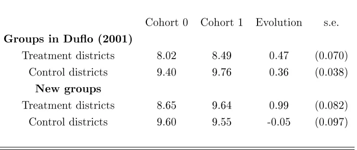
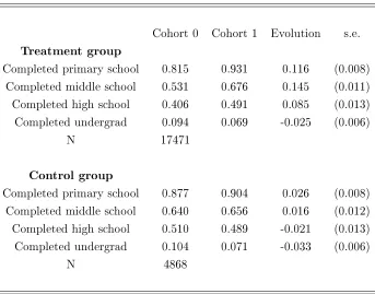
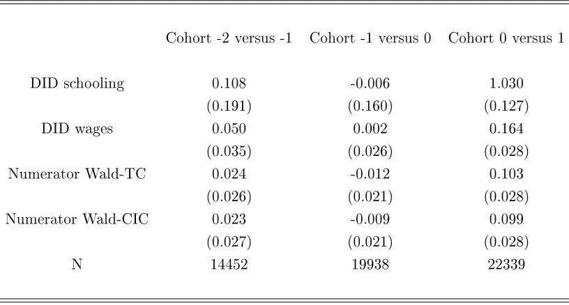
Finally, we use our results to revisit ndings in Duo (2001) on returns to education. The dis-tribution of schooling substantially changed in the control group used by the author, so using our Wald-CIC or Wald-TC estimators with her groups would only yield wide and uninforma-tive bounds. Therefore, we use a dierent control group where the distribution of schooling did not change. Our Wald-DID estimate with these new groups is more than twice as large as the author's. The dierence between these two estimates could stem from the fact that districts where years of schooling increased less also have higher returns to education. This would bias downward the estimate in Duo (2001), while our estimator does not rely on any treatment eect homogeneity assumption. On the other hand, the validity of our Wald-DID still relies on the assumption that time has the same eect on all potential outcomes, which is not warranted in this context as we explained above. Because the Wald-TC and Wald-CIC do not rely on this assumption, we choose them as our favorite estimates. They both lie in between the two Wald-DIDs.
Overall, our paper shows that to do DID in fuzzy designs, researchers must nd a control group in which treatment is stable over time to point identify treatment eects without having to assume that treatment eects are homogeneous. In such instances, three estimators are available: the standard Wald-DID estimator, and our Wald-TC and Wald-CIC estimators. While the former estimator requires that the eect of time be the same on all potential outcomes, the latter estimators do not rely on this assumption. In practice, using one or the other estimator can make a substantial dierence, as we show in our application.
Though to our knowledge, we are the rst to study fuzzy DID estimators in models with heterogeneous treatment eects, our paper is related to several other papers in the DID and panel literature. Blundell et al. (2004) and Abadie (2005) consider a conditional version of the common trends assumption in sharp DID designs, and adjust for covariates using propensity score methods. Our Wald-DID estimator with covariates is related to their estimators. Bon-homme & Sauder (2011) consider a linear model allowing for heterogeneous eects of time, and show that in sharp designs it can be identied if the idiosyncratic shocks are independent of the treatment and of the individual eects. Our Wald-CIC estimator builds on Athey & Imbens (2006) and is also related to the estimator of D'Haultf÷uille et al. (2013), who study the possibly nonlinear eects of a continuous treatment using repeated cross sections. Finally, Chernozhukov, Fernández-Val, Hahn & Newey (2013) consider a location-scale panel data model. Their idea of using always and never treated units in the panel to recover the location and scale parameters is related to our idea of using groups where treatment is stable to recover time eects.3 Our paper is also related to several papers in the partial identication literature.
3There are also dierences between our approaches (their model assumes time has the same eect on all
In particular, our bounds are related to those in Manski (1990), Horowitz & Manski (1995), and Lee (2009).
The remainder of the paper is organized as follows. In Section 2 we introduce our framework. In Section 3 we present our identication results in a simple setting with two groups, two periods, a binary treatment, and no covariates. Section 4 considers extensions to settings with many periods and groups, covariates, or a non-binary treatment. Section 5 considers inference. In section 6 we revisit results from Duo (2001). Section 7 concludes. The appendix gathers the main proofs. Due to a concern for brevity, some further results, our literature review, two supplementary applications, and additional proofs are deferred to our supplementary material (see de Chaisemartin & D'Haultf÷uille, 2015).
2 Framework
We are interested in measuring the eect of a treatmentD on some outcome. For now, we
assume that treatment is binary. Y(1)andY(0)denote the two potential outcomes of the same
individual with and without treatment. The observed outcome is Y =DY(1) + (1−D)Y(0).
We assume that the data at our disposal can be divided into time periods represented by a random variable T. If the analyst works with panel or repeated cross-sections data, time
periods are dates. But in many DID papers, time periods are cohorts of the same population born in dierent years (see, e.g., Duo, 2001). While with panel or repeated cross-sections data, each unit is or could be observed at both dates, with cohort data this is not the case. In what follows, we do not index observations by time, to ensure that our framework can apply to the three types of data. Referring to the panel data case is sometimes useful to convey the intuition of our results. However, our analysis is more targeted to the repeated cross-sections and cohort data cases: observing units at both dates open possibilities we do not explore here. We also assume that the data can be divided into groups represented by a random variable G.
In this section and in the next, we focus on the simplest possible case where there are only two groups, a treatment and a control group, and two periods of time. Gis a dummy for units
in the treatment group and T is a dummy for the second period. Contrary to the standard
sharp DID setting where D=G×T, we consider a fuzzy setting whereD6=G×T. Some
units may be treated in the control group or at period 0, and all units are not necessarily
treated in the treatment group at period 1. However, we assume that the treatment rate
increased more between period 0 and 1 in the treatment than in the control group.
We now introduce notations we use throughout the paper. For any random variable R, let
S(R) denote its support. Let also Rgt and Rdgt be two other random variables such that
Rgt ∼ R|G = g, T = t and Rdgt ∼ R|D = d, G = g, T = t, where ∼ denotes equality in
distribution. LetFRandFR|S denote the cumulative distribution function (cdfs) ofR and its
cdf conditional onS. For any event A,FR|A is the cdf of R conditional onA. With a slight
abuse of notation,P(A)FR|A should be understood as 0 whenP(A) = 0.
We consider the following model for the potential outcomes and the treatment:
Y(d) = hd(Ud, T), d∈ {0,1},
D = 1{V ≥vGT}, vG0 =v00 does not depend on G.
(1)
The model on potential outcomes is very general because at this stage,hdis left unrestricted.
We also impose a latent index model for the treatment (see, e.g., Vytlacil, 2002), where the threshold depends both on time and group. In such a model, V may be interpreted as the
propensity to be treated. Because we do not impose any restriction on the distribution ofV,
the assumption thatvG0 does not depend on Gis just a normalization.
In addition to this model, we maintain the following assumptions throughout the paper.
Assumption 1 (Time invariance within groups) For d∈ S(D), (Ud, V)⊥⊥T|G.
Assumption 2 (First stage)
E(D11)> E(D10), andE(D11)−E(D10)> E(D01)−E(D00).
Assumption 1 requires that the joint distribution of unobserved variables be stable over time in each group. In other words, the composition of each group should not change over time. This assumption could be violated if there is endogenous migration from one group to another. However, DID identication strategies always rely on this assumption. Beyond requiring that the treatment rates do not follow the exact same evolution in the two groups, Assumption 2 is just a way to dene the treatment and the control group in our fuzzy setting. First, the treatment should increase in at least one group. If not, one can redene the treatment variable asD˜ = 1−D. Then, the treatment group is the one experiencing the largest increase of its
treatment rate.
Before turning to identication, it is useful to dene four subpopulations of interest. The model 1 and Assumption 1 imply thatP(Dgt = 1) = P(V ≥ vgt|G=g). Therefore, Assumption 2
impliesv11< v00. Let
AT ={V ≥v00, G= 1} ∪ {V ≥max(v00, v01), G= 0},
N T ={V < v11, G= 1} ∪ {V <min(v00, v01), G= 0},
S1={V ∈[v11, v00), G= 1},
S0={V ∈[min(v00, v01),max(v00, v01)), G= 0}.
AT stands for always treated, and refers to units with a taste for treatment above the
treatment below the threshold at both periods. S1 stands for treatment group switchers,
and refers to treatment group units with a taste for treatment between the second and rst period thresholds. S0 stands for control group switchers, and refers to control group units
with a taste for treatment between the two thresholds.
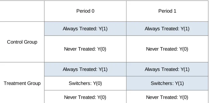
When the treatment rate is stable in the control group, time aects selection into treatment only in the treatment group. Table 1 below considers an example. At both dates, untreated units in the control group belong to the N T subgroup, while treated units belong to the AT
subgroup. On the other hand, untreated units in the treatment group in period 0 belong either to the N T or S1 subgroup, while in period 1 they only belong to the N T subgroup.
Conversely, treated units in period 0 only belong to theAT subgroup, while in period 1 they
either belong to theN T or S1 subgroup.
Never Treated: Y(0) Never Treated: Y(0)
Never Treated: Y(0) Always Treated: Y(1) Always Treated: Y(1)
Always Treated: Y(1)
Switchers: Y(0) Switchers: Y(1) Treatment Group
Control Group
Period 0 Period 1
Never Treated: Y(0)
[image:9.612.124.482.304.479.2]Always Treated: Y(1)
Table 1: Populations of interest whenP(D00= 0) =P(D01= 0).
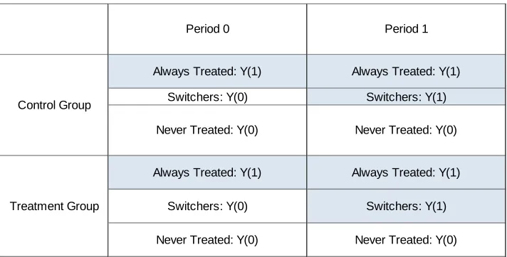
On the other hand, when the treatment rate changes in the control group, time aects selection into treatment in both groups. Table 2 below considers an example where the treatment rate increases in the control group. Untreated units in the control group in period 0 belong either to theN T or S0 subgroup, while in period 1 they only belong to theN T subgroup. Conversely,
treated units in period 0 only belong to theAT subgroup, while in period 1 they either belong
Switchers: Y(0) Switchers: Y(1)
Never Treated: Y(0)
Always Treated: Y(1)
Always Treated: Y(1)
Never Treated: Y(0)
Switchers: Y(0) Switchers: Y(1) Period 1
Control Group
Treatment Group
Period 0
Always Treated: Y(1)
Never Treated: Y(0)
Always Treated: Y(1)
[image:10.612.124.480.108.289.2]Never Treated: Y(0)
Table 2: Populations of interest whenP(D01= 1)> P(D00= 1).
Our identications results focus on treatment group switchers. Our parameters of interest are their Local Average Treatment Eect (LATE) and Local Quantile Treatment Eects (LQTE), which are respectively dened by
∆ = E(Y11(1)−Y11(0)|S1),
τq = FY−111(1)|S1(q)−FY−111(0)|S1(q), q∈(0,1).
We focus on this subpopulation because our assumptions either lead to point identication of
∆and τq, or at least to relatively tight bounds. On the other hand, our assumptions most
often lead to wide and uninformative bounds for the average treatment eect and for quantile treatment eects.
3 Identication
3.1 Identication using a Wald-DID ratio
We rst investigate the commonly used strategy of running an IV regression of the outcome on the treatment with time and group as included instruments, and the interaction of the two as the excluded instrument. The estimand arising from this regression is the Wald-DID dened byWDID=DIDY/DIDD where, for any random variable R, we let
DIDR=E(R11)−E(R10)−(E(R01)−E(R00)).
We consider a set of assumptions under which this estimand can receive a causal interpretation.
Assumption 3 (Common trends)
Assumption 4 (Common average eect of time on both potential outcomes)
E(h1(U1,1)−h1(U1,0)|G, V ≥v00) =E(h0(U0,1)−h0(U0,0)|G, V ≥v00).
Assumption 3 requires that the mean of Y(0) follow the same evolution over time in the
treatment and control groups. This assumption is not specic to the fuzzy setting we are considering here: DID in sharp settings also rely on this assumption (see, e.g., Abadie, 2005). Assumption 4 requires that in both groups, the mean of Y(1) and Y(0) follow the same
evolution over time among units treated in period0. This is equivalent to assuming that the
average treatment eect in this population does not change over time. This assumption is specic to the fuzzy setting.
Theorem 3.1 Assume that Model (1) and Assumptions 1-4 are satised. Letα= P(D11=1)−P(D10=1)
DIDD .
1. IfP(D01= 1)≥P(D00= 1), α≥1 and
WDID=αE(Y11(1)−Y11(0)|S1)−(α−1)E(Y01(1)−Y01(0)|S0).
2. IfP(D01= 1)< P(D00= 1), α <1 and
WDID=αE(Y11(1)−Y11(0)|S1) + (1−α)E(Y00(1)−Y00(0)|S0).
When the treatment rate increases in the control group, the Wald-DID is equal to a weighted dierence of two LATEs. This can be seen from Table 2. In both groups, the evolution of the mean outcome between period 0 and 1 is the sum of three things: the eect of time on the mean ofY(0) for never treated and switchers; the eect of time on the mean ofY(1) for
always treated; the average eect of the treatment for switchers. Under Assumptions 3 and 4, the eect of time in both groups cancel one another out. The Wald-DID is nally equal to the weighted dierence between treatment and control group switchers' LATEs.
This weighted dierence may not receive a causal interpretation. It might for instance be negative, while both E(Y11(1)−Y11(0)|S1) and E(Y01(1)−Y01(0)|S0) are positive. If one
is ready to further assume that these two LATEs are equal, the Wald-DID is then equal to
E(Y11(1)−Y11(0)|S1). ButE(Y11(1)−Y11(0)|S1) =E(Y01(1)−Y01(0)|S0)is a strong restriction
on the heterogeneity of the treatment eect. To better understand why it is needed, let us consider a simple example in which all control group units have a treatment eect equal to
+2, while all treatment group units have a treatment eect equal to +1. Let us also assume
that time has no eect on the outcome, and that the treatment rate increases twice as much in the treatment than in the control group. Then,WDID = 2/3×1−1/3×2 = 0: the lower
When the treatment rate diminishes in the control group, the Wald-DID is equal to a weighted average of LATEs. This quantity is not straightforward to interpret, because it aggregates the LATE of treatment group switchers in period 1 and the LATE of control group switchers in period 0. But it satises the no sign-reversal property: if the treatment eect is of the same sign for everybody in the population, the Wald-DID is of that sign. Moreover, under the assumption that control group switchers' LATE does not change between period 0 and 1, this weighted average rewrites asE(Y(1)−Y(0)|S1∪S0, T = 1).
Finally, when the treatment rate is stable over time in the control group, the Wald-DID is equal to the LATE of treatment group switchers. Indeed, in such instances we haveα= 1, so
the rst statement of the theorem simplies into WDID= ∆.
But even when the treatment rate is stable in the control group, the Wald-DID relies on the assumption that time has the same eect on both potential outcomes, at least among units treated in the rst period. Under Assumptions 1-3 alone, one can show that WDID is equal
to the same quantity as in Theorem 3.1, plus a bias term equal to
1 DIDD
[E(C1−C0|V ≥v00, G= 1)P(D10= 1)−E(C1−C0|V ≥v00, G= 0)P(D00= 1)],
where Cd = hd(Ud,1)−hd(Ud,0). Assumption 5 ensures that this bias term is equal to 0.
Otherwise, it might very well dier from 0.4
To better understand why this restriction is needed, consider a simple example where time increasesY(1)by 1 unit, while leavingY(0) unchanged. Assume also that in period 0,
treat-ment had no eect. Finally, assume that the treattreat-ment rate went from to 20 to 50% in the treatment group, while it remained equal to 80% in the control group. Then, DIDY =
0.2×1+0.3×1+0.5×0−(0.8×1+0.2×0) =−0.3. The rst and third terms respectively come
from the eect of time on always and never treated in the treatment group. Similarly, the fourth and fth terms respectively come from the eect of time on always and never treated in the control group. Finally, the second term comes from the treatment eect among treatment group switchers. Therefore,WDID=−1, while every unit in the population has a treatment
eect equal to1 in period 1, and to0 in period 0.
The assumption that time has homogeneous eects on both potential outcomes might not always be plausible. For instance, the relative earnings of college graduates in the US in-creased dramatically in the 1980s (see Katz et al., 1999), suggesting that time might have had heterogeneous eects on potential wages with and without a college degree.
3.2 Identication using a time-corrected Wald ratio
In this section, we consider a rst set of alternative estimands toWDID. Instead of relying on
Assumptions 3 and 4, they rely on the following assumption:
4Assuming that E(C
0−C1|V < v0, G) does not depend on Gis not sucient to ensure that the bias is
Assumption 5 (Common trends within treatment status at date 0)
E(h0(U0,1)−h0(U0,0)|G, V < v00) and E(h1(U1,1)−h1(U1,0)|G, V ≥ v00) do not depend
on G.
Assumption 5 requires that the mean ofY(0)(resp. Y(1)) follow the same evolution over time
among treatment and control group units that were untreated (resp. treated) at period0.
Letδd=E(Yd01)−E(Yd00) denote the change in the mean outcome between period 0 and 1
for control group units with treatment statusd. Then, let
WT C =
E(Y11)−E(Y10+δD10)
E(D11)−E(D10) .
WT C stands for time-corrected Wald.
When the outcome is bounded, letyandy respectively denote the lower and upper bounds of
its support. For anyg∈ S(G), let λgd=P(Dg1 =d)/P(Dg0 =d) be the ratio of the shares of
people receiving treatment din period 1 and period 0 in groupg. For instance,λ00>1when
the share of untreated observations increases in the control group between period 0 and 1. For any real number x, let M0(x) = max(0, x) and m1(x) = min(1, x). Let also, for d∈ {0,1},
Fd01(y) =M0[1−λ0d(1−FYd01(y))]−M0(1−λ0d)1{y < y},
Fd01(y) =m1[λ0dFYd01(y)] + (1−m1(λ0d))1{y≥y}.
Then deneδd=R ydFd01(y)−E(Yd00) andδd=
R
ydFd01(y)−E(Yd00) and let
WT C = E(Y11)−E(Y10+δD10)
E(D11)−E(D10)
, WT C =
E(Y11)−E(Y10+δD10)
E(D11)−E(D10) .
Theorem 3.2 Assume that Model (1) and Assumptions 1-2 and 5 are satised.
1. If0< P(D01= 1) =P(D00= 1)<1, WT C = ∆.
2. If 0 < P(D01 = 1) 6= P(D00 = 1) < 1 and P(y ≤ Y(d) ≤ y) = 1 for d ∈ {0,1}, WT C ≤∆≤WT C.5
Our point identication result extends the DID logic to fuzzy settings. We seek to recover the mean of, say, Y(1) among switchers in the treatment × period 1 cell. On that purpose,
we start from the mean ofY among all treated observations of this cell. As shown in Table
1, those include both switchers and always treated. Consequently, we must withdraw the mean ofY(1)among always treated. This quantity is not observed. To reconstruct it, we add
to the mean of Y(1)among always treated of the treatment group in period 0 the evolution of
the mean of Y(1)among always treated of the control group between period 0 and 1. We use
similar steps to recover the mean ofY(0) among switchers in the treatment×period 0 cell.
Note that
WT C =
E(Y|G= 1, T = 1)−E(Y + (1−D)δ0+Dδ1|G= 1, T = 0) E(D|G= 1, T = 1)−E(D|G= 1, T = 0) .
This is almost the Wald ratio with time as the instrument considered rst by Heckman & Robb (1985), except that we have Y + (1−D)δ0+Dδ1 instead of Y in the second term of
the numerator. This dierence arises because time is not a standard instrument: it is directly included in the outcome equation. When the treatment rate is stable in the control group we can identify the direct eect of time onY(0)and Y(1) by looking at how the mean outcome
of untreated and treated units changes over time in this group. Under Assumption 5, this direct eect is the same in the two groups for units sharing the same treatment status in the rst period. As a result, we can add these changes to the outcome of untreated and treated units in the treatment group in period0, to recover the mean outcome we would have
observed in this group in period1 if time had not aected selection into treatment. This is
what (1−D)δ0+Dδ1 does. Therefore, the numerator ofWT C is equal to the eect of time
on the outcome which only goes through its eect on selection into treatment. Once properly normalized, this yields the LATE of treatment group switchers.
When the treatment rate changes in the control group, the evolution of the outcome in this group can stem both from the direct eect of time on the outcome, and from its eect on selection into treatment. For instance, and as can be seen from Table 2, when the treatment rate increases in the control group, the dierence between E(Y101) and E(Y100) arises both
from the eect of time onY(1), and from the fact the former expectation is for always treated
and switchers while the later is only for always treated. Therefore, we can no longer identify the direct eect of time on the outcome. However, when the outcome has bounded support, this direct eect can be bounded, because we know the percentage of the control group switchers account for. As a result, the LATE of treatment group switchers can also be bounded. The smaller the change of the treatment rate over time in the control group, the tighter the bounds. When the treatment rate does not change much in the control group, the dierence between
WT C and ∆ is likely to be small. For instance, when the treatment rate increases in the
control group, it is easy to show that under the Assumptions of Theorem 3.2, WT C is equal
to∆plus the following bias term:
P(D10= 0)
1−P(D01=0)
P(D00=0)
(E(Y01(0)|S0)−E(Y01(0)|N T))
P(D11= 1)−P(D10= 1)
−
P(D10= 1)
1−P(D00=1)
P(D01=1)
(E(Y01(1)|S0)−E(Y01(1)|AT))
P(D11= 1)−P(D10= 1)
. (2)
This term cancels ifP(D01= 1) =P(D00= 1), but also if
This assumption is not very appealing, as it requires that control group switchers have the same distribution of U0 as never treated, and the same distribution of U1 as always treated.
But Equations (2) and (3) still show that when the treatment rate does not change much in the control group,WT C is close to∆unless switchers are extremely dierent from never and
always treated.
Finally, note that when the treatment rate is stable in the control group, we have
WDID=
E(Y11)−E(Y10+δD00)
E(D11)−E(D10) .
When accounting for the eect of time on the outcome,WDIDweightsδ0andδ1byP(D00= 0)
andP(D00= 1), whileWT C weights these terms by P(D10= 0) andP(D10= 1). These two
estimands are equal if and only if eitherδ0 =δ1 or P(D00 = 1) = P(D10 = 1). Otherwise,
they dier. The assumptions under whichWDIDandWT C rely are non-nested. WT C requires
more common trends assumptions between groups, but it does not require common trends assumptions between the two potential outcomes within groups. Therefore, testingWDID =
WT C is a joint test of Assumptions 1 and 3-5.
3.3 Identication using instrumented changes-in-changes
In this section, we consider a second set of alternative estimands for continuous outcomes, inspired from the CIC model in Athey & Imbens (2006). These estimands crucially rely on a monotonicity assumption.
Assumption 6 (Monotonicity)
Ud∈R andhd(u, t) is strictly increasing inu for all (d, t)∈ S(D)× S(T).
Assumption 6 requires that at each period, potential outcomes are strictly increasing functions of a scalar unobserved heterogeneity term. Hereafter, we refer to Assumptions 1-2 and 6 as to the IV-CIC model. The IV-CIC model generalizes the CIC model to fuzzy settings. Assumption 1 implies Ud ⊥⊥ T|G and V ⊥⊥ T|G, which correspond to the time invariance
assumption in Athey & Imbens (2006). As a result, the IV-CIC model imposes a standard CIC model both on Y and D. But Assumption 1 also implies Ud ⊥⊥T|G, V: in each group, the
distribution of, say, ability among people with a given taste for treatment should not change over time. Our results rely on this supplementary restriction.
the treatment group among any quantile group of the always treated remains constant over time. For instance, if, in period 0, 70% of units in the rst decile of always treated belonged to the treatment group, in period 1 there should still be 70% of treatment group units in the rst decile. This condition is invariant to the scaling of the outcome, but it restricts its entire distribution. When the treatment and the control groups have dierent outcome distributions in the rst period (see e.g. Baten et al., 2014), the scaling of the outcome might have a large eect on the results, so using a model invariant to this scaling might be preferable. On the other hand, when the outcome distributions in the treatment and in the control group are similar in the rst period, using a model that only restricts the rst moment of the outcome might be preferable.
We also impose the assumption below, which is testable in the data.
Assumption 7 (Data restrictions)
1. S(Ydgt) =S(Y) = [y, y]with −∞ ≤y < y ≤+∞, for (d, g, t)∈ S(D)× S(G)× S(T).
2. FYdgt is continuous on Rand strictly increasing on S(Y), for(d, g, t)∈ S(D)× S(G)×
S(T).
The rst condition requires that the outcome have the same support in each of the eight treatment×group×period cell. This condition does not restrict the support to be bounded:
y and y can be equal to − and +∞. Athey & Imbens (2006) make a similar assumption.
Common support conditions might not be satised when outcome distributions dier in the treatment and in the control group, the very situations where CIC might be more appealing than DID. Athey & Imbens (2006) show that in such instances, quantile treatment eects are still point identied over a large set of quantiles, while the average treatment eect can be bounded. Even though we do not present them here, similar results apply in fuzzy settings. The second condition is satised if the distribution ofY is continuous with positive density in
each of the eight groups×periods×treatment status cells. With a discrete outcome, Athey
& Imbens (2006) show that one can bound treatment eects under their assumptions. Similar results apply in fuzzy settings, but as CIC bounds for discrete outcomes are often not very informative, we do not present them here.
Let Qd(y) = FY−d101 ◦FYd00(y) be the quantile-quantile transform of Y from period 0 to 1
in the control group conditional on D = d. This transform maps y at rank q in period 0
into the corresponding y0 at rank q in period 1. Let also Hd(q) = FYd10 ◦F
−1
Yd00(q) be the
inverse quantile-quantile transform ofY from the control to the treatment group in period 0
conditional onD=d. This transform maps rankq in the control group into the corresponding
rankq0 in the treatment group with the same value ofy. Finally, for any increasing function F on the real line, we denote byF−1 its generalized inverse:
In particular, FX−1 is the quantile function of X. We adopt the convention that FX−1(q) = infS(X) for q <0, and FX−1(q) = supS(X)for q >1.
Our identication results rely on the following lemma.
Lemma 3.1 If Assumptions 1-2 and 6-7 hold and if P(D00=d)>0,
FY11(d)|S1(y) =
P(D10=d)Hd◦(λ0dFYd01(y) + (1−λ0d)FY01(d)|S0(y))−P(D11=d)FYd11(y)
P(D10=d)−P(D11=d)
.
This lemma shows that under our IV-CIC assumptions,FY11(d)|S1 is point identied when the
treatment rate remains constant in the control group, as in this caseλ0d= 1. Let
FCIC,d(y) =
P(D10=d)Hd◦(FYd01(y))−P(D11=d)FYd11(y)
P(D10=d)−P(D11=d)
WCIC =
E(Y11)−E(QD10(Y10))
E(D11)−E(D10) .
When the treatment rate changes in the control group,FY11(d)|S1 is partially identied. Sharp
bounds can be obtained using Lemma 3.1. For any cdf Td, let
Gd(Td) =λ0dFYd01+ (1−λ0d)Td
Cd(Td) =
P(D10=d)Hd◦Gd(Td)−P(D11=d)FYd11
P(D10=d)−P(D11=d)
.
It follows from Lemma 3.1 that Cd(FY11(d)|S0) = FY11(d)|S1. Moreover, one can show that
G0(FY11(0)|S0) = FY01(0)|V <v00 and G1(FY11(1)|S0) = FY01(1)|V≥v00. Therefore, the sharp lower
bound onFY11(d)|S1 is
min
Td∈D
Cd(Td) s.t. (Td, Gd(Td), Cd(Td))∈ D3,
whereDis the set of cdfs onS(Y).
Unfortunately, it is dicult to derive a closed form expression for the solution of this problem, because it corresponds to an innite dimensional optimization problem with an innite number of inequality constraints. We therefore consider simpler bounds, which are sharp under a simple testable assumption. Specically, letM01(x) = min(1,max(0, x)), and let
Td=M01
λ0dFYd01−H
−1
d (λ1dFYd11)
λ0d−1
!
, Td=M01
λ0dFYd01−H
−1
d (λ1dFYd11+ (1−λ1d))
λ0d−1
!
,
FCIC,d(y) = sup
y0≤y
Cd(Td) (y 0), F
CIC,d(y) = inf
y0≥yCd Td
(y0),
WCIC =
Z
ydFCIC,1(y)−
Z
ydFCIC,0(y), WCIC =
Z
ydFCIC,1(y)−
Z
ydFCIC,0(y),
τq= max(F−CIC,1 1(q), y)−min(FCIC,−1 0(q), y), τq= min(F−CIC,1 1(q), y)−max(F −1
CIC,0(q), y).
Assumption 8 (Existence of moments)
R
|y|dFCIC,d(y)<+∞ and
R
|y|dFCIC,d(y)<+∞ for d∈ {0,1}.
Assumption 9 (Increasing bounds) For (d, g, t) ∈ S(D)× {0,1}2, F
Ydgt is continuously dierentiable, with positive derivative on
the interior ofS(Y). Moreover,Td, Td, Gd(Td), Gd(Td), Cd(Td) andCd(Td)are increasing on S(Y).
Theorem 3.3 Assume that Model (1) and Assumptions 1-2 and 6-7 hold.
1. If 0 < P(D01 = 1) = P(D00 = 1) < 1, then FCIC,d(y) = FY11(d)|S1(y) for d ∈ {0,1},
WCIC = ∆ and FCIC,−1 1(q)−F
−1
CIC,0(q) =τq.
2. If0< P(D01= 1)6=P(D00= 1)<1 and Assumption 8 is satised, thenFY11(d)|S1(y)∈
[FCIC,d(y), FCIC,d(y)] for d∈ {0,1}, ∆∈[WCIC, WCIC] and τq ∈[τq, τq]. Moreover,
if Assumption 9 holds, these bounds are sharp.
Our point identication results combine ideas from Imbens & Rubin (1997) and Athey & Imbens (2006). We seek to recover the distribution of, say, Y(1) among switchers in the
treatment × period 1 cell. On that purpose, we start from the distribution of Y among all
treated observations of this cell. As shown in Table 1, those include both switchers and always treated. Consequently, we must withdraw from this distribution that ofY(1)among always
treated, exactly as in Imbens & Rubin (1997). But this last distribution is not observed. To reconstruct it, we adapt the ideas in Athey & Imbens (2006) and apply the quantile-quantile transform from period 0 to 1 among treated observations in the control group to the distribution ofY(1)among treated units in the treatment group in period 0.
Intuitively, the quantile-quantile transform uses a double-matching to reconstruct the unob-served distribution. Consider an always treated in the treatment ×period 0 cell. She is rst
matched to an always treated in the control× period 0 cell with same y. Those two always
treated are observed at the same period of time and are both treated. Therefore, under As-sumption 6 they must have the same u1. Second, the control × period 0 always treated is
matched to her rank counterpart among always treated of the control × period 1 cell. We
denote y∗ the outcome of this last observation. BecauseU1 ⊥⊥T|G, V ≥v00, those two
ob-servations must also have the same u1. Consequently,y∗ =h1(u1,1), which means that y∗ is
the outcome that the treatment× period 0 cell unit would have obtained in period 1.
Note that
WCIC =
E(Y|G= 1, T = 1)−E((1−D)Q0(Y) +DQ1(Y)|G= 1, T = 0) E(D|G= 1, T = 1)−E(D|G= 1, T = 0) .
Here again, WCIC is almost the standard Wald ratio in the treatment group with T as the
of the numerator. (1−D)Q0(Y) +DQ1(Y) accounts for the fact time has a direct eect on
the outcome. When the treatment rate is stable in the control group, we can identify this direct eect by looking at how the distribution of the outcome evolves in this group. We can then net out this direct eect in the treatment group. This is what(1−D)Q0(Y) +DQ1(Y)
does. Both WCIC and WT C proceed from the same logic, except that WT C corrects for
the eect of time through additive shifts, while WCIC does so in a non-linear fashion. If
hd(Ud, T) = ad(Ud) +bd(T) with ad(.) strictly increasing, Assumptions 5 and 6 are both
satised. We then have WCIC =WT C.
Our partial identication results are obtained as follows. When 0< P(D00 = 1)6=P(D01= 1) < 1, the second matching described above collapses, because treated (resp. untreated)
observations in the control group are no longer comparable in period 0 and 1. For instance, when the treatment rate increases in the control group, treated observations in the control group include only always treated in period 0. In period 1 they also include switchers, as is shown in Table 2. Therefore, we cannot match period 0 and period 1 observations on their rank anymore. However, under Assumption 1 the respective weights of switchers and always treated in period 1 are known. We can therefore derive best and worst case bounds for the distribution of the outcome for always treated in period 1, and match period 0 observations to their best and worst case rank counterparts.
If the support of the outcome is unbounded, FCIC,0 andFCIC,0 are proper cdf whenλ00>1,
but they are defective when λ00<1. Whenλ00<1, switchers belong to the group of treated
observations in the control × period 1 cell (cf. Table 2). Their Y(0) is not observed in
period 1, so the data does not impose any restriction on FY01(0)|S0: it could be equal to 0 or
to 1, hence the defective bounds. On the contrary, when λ00 > 1, switchers belong to the
group of untreated observations in the control × period 1 cell, and under Assumption 1 we
know that they account for 100(1−1/λ00)of this group. Consequently, we can use trimming
bounds forFY01(0)|S0 (see Horowitz & Manski, 1995), hence the non-defective bounds. On the
contrary, FCIC,1 and FCIC,1 are always proper cdf, while we could have expected them to
be defective when λ00>1. This asymmetry stems from the fact that when λ00 >1, setting FY01(1)|S0(y) = 0 would yield FY01(1)|S1(y) > 1 for values of y approaching y, while setting
FY01(1)|S0(y) = 1would yield FY01(1)|S1(y)<0 for values of y approaching y.
The previous discussion implies that whenS(Y) is unbounded andλ00<1, our bounds on∆
are innite because our bounds for the cdf of Y(0) of switchers are defective. Our bounds on τqare also innite for low and high values of q. On the contrary, whenλ00>1our bounds on τq are nite for everyq∈(0,1). Our bounds on∆are also nite providedFCIC,0 andFCIC,0
admit an expectation.
3.4 Identication with a fully treated or fully untreated control group
Up to now, we have considered general fuzzy situations where theP(Dgt=d) were restricted
only by Assumption 2. An interesting special case, which is close to the sharp design, is when
P(D00= 1) =P(D01= 1) =P(D10= 1) = 0. In such instances, identication of the average
treatment eect on the treated can be obtained under the same assumptions as those of the standard DID or CIC models.
Theorem 3.4 Suppose that P(D00 = 1) = P(D01 = 1) = P(D10 = 1) = 0 < P(D11 = 1), U0⊥⊥T|G, and the outcome equation of Model (1) is satised.
1. If Assumption 3 holds, thenWDID=WT C =E(Y11(1)−Y11(0)|D= 1).
2. If Assumptions 6 and 7 hold, then WCIC =E(Y11(1)−Y11(0)|D= 1).
Hence, results of the sharp case extend to this intermediate case. Note that under Model (1) and Assumption 1, the treated population corresponds toS1, soE(Y11(1)−Y11(0)|D= 1) = ∆
under these additional assumptions.
Another special case of interest is when P(D00 = 0) =P(D01= 0) ∈ {0,1}. Such situations
arise, for instance when a policy is extended to a previously a group, or when a program or a technology previously available in some geographic areas is extended to others (see our second supplementary application in de Chaisemartin & D'Haultf÷uille (2015)). Theorem 3.1 applies in this special case, but not Theorems 3.2-3.3, as they require that0< P(D00= 0) =P(D01= 0)<1. In such instances, identication must rely on the assumption that time has the same
eect on both potential outcomes. For instance, if P(D00 = 1) = P(D01 = 1) = 1 and P(D10 = 1)<1, there are no untreated units in the control group which we can use to infer
trends for untreated units in the treatment group. We must therefore use treated units, under the assumption that time has the same eect on both potential outcomes. Instead of the Wald-TC estimand, one could then use E(Y11)−E(Y10+δ1)
E(D11)−E(D10) . Because P(D00 = 1) =P(D01 = 1) = 1,
this actually amounts to using WDID instead of WT C. We can also adapt our Wald-CIC
estimand by considering the following assumption.
Assumption 10 (Common eect of time on both potential outcomes)
h0(h−01(y,0),1) =h1(h1−1(y,0),1)for every y∈ S(Y).
a structural function satisfying Assumption 10 is hd(Ud, T) = f(gd(Ud), T) with f(., t) and
gd(.) strictly increasing. This shows that Assumption 10 does not restrict the eects of time
and treatment to be homogeneous. Finally, Assumptions 4 and 10 are related, but they also dier on some respects. Assumption 4 restricts time to have the same average eect on the potential outcomes of always treated. Assumption 10 restricts time to have the same eect on the potential outcomes of units satisfyingY(0) =Y(1)at the rst period.
Under assumption 10, ifP(D00=d) =P(D01=d) = 1we can use changes in the distribution
ofY(d)in the control group over time to identify the eect of time onY(1−d), hence allowing
us to recover both FY11(d)|S1 and FY11(1−d)|S1.
Theorem 3.5 If Assumptions 1-2, 6-7, and 10 hold, and P(D00=d) =P(D01=d) = 1 for
some d∈ {0,1},
P(D10=d)FQd(Yd10)(y)−P(D11=d)FYd11(y)
P(D10=d)−P(D11=d)
=FY11(d)|S1(y),
P(D10= 1−d)FQd(Y1−d10)(y)−P(D11= 1−d)FY1−d11(y)
P(D10= 1−d)−P(D11= 1−d)
=FY11(1−d)|S1(y),
E(Y11)−E(Q1−d(Y10)) E(D11)−E(D10)
= ∆.
The estimands introduced in this theorem are very similar to those considered in the rst point of Theorem 3.3, except that they apply the same quantile-quantile transform to all treatment units in period 0, instead of applying dierent transforms to units with a dierent treatment. Finally, when0< P(D00= 1) =P(D01= 1)<1, Assumption 10 is testable. If it is satised,
the quantile-quantile transforms Q0 and Q1 must be equal. When this test is not rejected,
applying a weighted average of these two transforms to all treatment group units in period 0 might result in eciency gains with respect to our Wald-CIC estimator.
3.5 Panel data models
Model (1) is well suited for repeated cross sections or cohort data where we observe units only once. On the other hand, it implies a strong restriction on selection into treatment when panel data are available. AsV does not depend on time, our selection equation implies that within
each group, time can aect individuals' treatment decision in only one direction. Actually, all our results would remain valid if Ud andV were indexed by time, except that we would have
to rewrite Assumption 1 as follows: for d ∈ S(D), the distribution of (Udt, Vt)|G does not
depend ont. Within each group, time could then induce some units to go from non-treatment
to treatment, while having the opposite eect on other units.
We now discuss whether the common trends and monotonicity assumptions we introduced above are satised in standard panel data models. We index random variables byi, to
First, we consider the following model:
Yit=γt+αi+βiDit+εit, (4)
Dit= 1{Vit≥vgt}, (5)
(εi1, Vi1, αi, βi)|Gi ∼(εi0, Vi0, αi, βi)|Gi. (6)
The outcome equation has time and individual eects. It allows for heterogeneous but time invariant treatment eects which can be arbitrarily correlated with the treatment, the xed eects, and the idiosyncratic shocks. Equation (6) requires that the distribution of
(εit, Vit, αi, βi)|Gi does not depend on time. On the other hand, it does not restrict the
cross-sectional dependence between εit and Vit, nor serial dependence between (εi0, Vi0) and (εi1, Vi1). This implies in particular that in the rst-dierence equation,Di1−Di0 is
endoge-nous in general. The Wald-DID estimand then amounts to instrument Di1−Di0 byGiin this
rst-dierence equation. It is easy to see that if Equations (4)-(6) hold, then Assumptions 1-5 are satised:6 the additive time eect and the time invariant treatment eect ensure that
Assumptions 3, 4 and 5 are satised. Hence, both the Wald-DID and the Wald-TC estimands are equal to∆.
Second, we consider the following outcome equation instead of Equation (4):
Yit=γt+λtDit+αi+βiDit+εit. (7)
Under Equation (7), Assumption 4 is no longer satised because treatment eects change over time. On the other hand, the eect of time on both potential outcomes is still additive, so Equations (7) and (5)-(6) guarantee that Assumptions 1-2 and 5 are satised. Hence, the Wald-TC estimand is equal to ∆.
Then, we consider the following outcome equation:
Yit=γt+λtDit+µt(αi+βiDit+εit). (8)
Under Equation (8), Assumption 4 is no longer satised because time has an heterogeneous eect on the outcome. On the other hand, if Equations (8) and (5)-(6) hold, then Assumptions 1-2 and 6 are satised. To see this, dene hd(u, t) =γt+λtd+µtu andUdit=αi+βid+εit.
Finally, we consider a last outcome equation:
Yit=γt+λtDit+αi+βiDit+µtεit. (9)
All our assumptions fail to hold under this xed eects model with time-varying eects of the idiosyncratic shock. As above, Assumption 4 fails because time has heterogeneous eects
6U
dandV should be indexed by time, and Assumption 1 should be rewritten as follows: ford∈ S(D), the
on the outcome. Assumption 6 also fails because the outcome can no longer be written as a function of time and a scalar unobserved term. Bonhomme & Sauder (2011) study a similar model with xed eects and non-stationary idiosyncratic shocks. In the sharp case, they show that average and quantile treatment eects are identied if the idiosyncratic shocks are independent of treatment and of the xed eects.
4 Extensions
In this section, we extend our analysis to situations where the data can be divided into several groups and several periods, where covariates are available, or where the treatment is non-binary. To generalize our results, we have to modify some of the assumptions we introduced above. To ease the comparison, we label these assumptions using suxes. For instance Assumption 1X is similar to Assumption 1 except that it accounts for covariatesX.
4.1 Multiple groups and time periods
Let us consider the case where the data can be divided into more than two groups and time periods. Let G ∈ {0,1, ..., g} be the group a unit belongs to. Let T ∈ {0,1, ..., t}
be the period when she is observed. For any (g, t) ∈ S(G)× {1, ..., t}, let Sgt = {V ∈
[min(vgt−1, vgt),max(vgt−1, vgt)), G = g} be the subset of group g which switches treatment
status betweent−1 and t. Also, letSt =∪gg=0Sgt denote the units switching between t−1
and t. Finally, let S =St
t=1St be the union of all switchers. At each date, we can partition
the groups into three subsets, depending on whether their treatment rate is stable, increases, or decreases betweent−1and t. For every t∈ {1, ..., t}, let
Gst ={g∈ S(G) :E(Dgt) =E(Dgt−1)}
Git={g∈ S(G) :E(Dgt)> E(Dgt−1)}
Gdt ={g∈ S(G) :E(Dgt)< E(Dgt−1)},
and let G∗t = 1{G ∈ Git} −1{G ∈ Gdt}. We introduce the following assumptions, which
generalize Assumptions 3-5 to settings with multiple groups and periods (Assumptions 6 and 7 apply to this case without modications).
Assumption 3M (Common trends)
For every t∈ {1, ..., t}, E(h0(U0, t)−h0(U0, t−1)|G) does not depend onG.
Assumption 4M (Common average eect of time on both potential outcomes)
Assumption 5M (Common trends within treatment at previous period)
For everyt∈ {1, ..., t}, E(h0(U0, t)−h0(U0, t−1)|G, V < vGt−1)andE(h1(U1, t)−h1(U1, t− 1)|G, V ≥vGt−1) do not depend on G.
Theorem 4.1 below shows that when there is at least one group in which the treatment rate is stable between each pair of consecutive dates, combinations of these assumptions allow us to point identify∆w, a weighted average of LATEs over dierent periods:
∆w = t
X
t=1
P(St|T =t)
Pt
t=1P(St|T =t)
E(Y(1)−Y(0)|St, T =t).
We also consider the following assumption, under which∆w is equal to the LATE among the
whole population of switchersS.
Assumption 11 (Stable groups, monotonic evolution of treatment, and homogenous eects over time)
1. G⊥⊥T.
2. For every t6=t0 ∈ {1, ..., t}2 G
it∩ Gdt0 =∅.
3. For every (t, t0)∈ {1, ..., t}2, E(Y(1)−Y(0)|S
t, T =t0) =E(Y(1)−Y(0)|St, T = 1).
The rst point of Assumption 11 requires that the distribution of groups be stable over time. This will automatically be satised if the data is a balanced panel and G is time invariant.
With repeated cross-sections or cohort data, this assumption might fail to hold. However, large deviations from this stable group assumption indicate that some groups grow much faster than others, which might anyway call into question the common trends assumptions underlying DID identication strategies. The second point of Assumption 11 requires that in every group, the treatment rate follows a monotonic evolution over time. The third point requires that switchers' LATE be homogeneous over time.
For any random variable R and for any (g, t) ∈ {−1,0,1} × S(T), let R∗gt∼R|G∗t =g, T =t
and R∗dgt∼R|D=d, G∗t =g, T =t. For any g6=g0∈ {−1,0,1}2 andt∈ {1, ..., t}let
DID∗R(g, g0, t) =E(R∗gt)−E(R∗gt−1)−(E(R
∗
g0t)−E(R∗g0t−1))
WDID∗ (g, g0, t) = DID
∗ Y(g, g
0, t)
DID∗D(g, g0, t)
wt=
DIDD∗(1,0, t)P(G∈ Git|T =t) +DIDD∗(0,−1, t)P(G∈ Gdt|T =t)
Pt
t=1DID∗D(1,0, t)P(G∈ Git|T =t) +DID ∗
D(0,−1, t)P(G∈ Gdt|T =t)
w01|t=
DID∗D(1,0, t)P(G∈ Git|T =t)
Let also
δdt∗ =E(Yd∗0t)−E(Yd∗0t−1) for d∈ {0,1}
WT C∗ (1,0, t) =
E(Y1∗t)−E(Y1∗t−1+δD∗∗
1t−1)
E(D∗1t)−E(D1∗t−1)
WT C∗ (−1,0, t) =
E(Y−∗1t)−E(Y−∗1t−1+δ∗D∗ −1t−1)
E(D∗−1t)−E(D−∗1t−1) .
Finally, let
Q∗dt(y) =FY−∗1
d0t
◦FYd∗0t−1(y) d∈ {0,1}
WCIC∗ (1,0, t) =
E(Y1∗t)−E(Q∗D∗
1t−1(Y
∗
1t−1)) E(D1∗t)−E(D1∗t−1)
WCIC∗ (−1,0, t) =
E(Y−∗1t)−E(Q∗D∗−1t−1(Y
∗ −1t−1)) E(D−∗1t)−E(D∗−1t−1) .
Theorem 4.1 Assume that Model (1) and Assumption 1 are satised. Assume also that for every t∈ {1, ..., t}, Gst6=∅.
1. If Assumptions 3M and 4M are satised,
t
X
t=1
wt(w10|tWDID∗ (1,0, t) + (1−w10|t)WDID∗ (−1,0, t)) =∆w.
2. If Assumption 5M is satised,
t
X
t=1
wt(w10|tWT C∗ (1,0, t) + (1−w10|t)WT C∗ (−1,0, t)) =∆w.
3. If Assumptions 6 and 7 are satised,
t
X
t=1
wt(w10|tWCIC∗ (1,0, t) + (1−w10|t)WCIC∗ (−1,0, t)) =∆w.
4. If either t= 1 or Assumption 11 holds,
∆w =E(Y(1)−Y(0)|S, T >0).
Let us rst consider the simple case with multiple groups and two periods. In such instances, the rst, second, and third results of the theorem can respectively be rewritten as
This shows that with multiple groups and two periods of time, treatment eects for switchers are identied if there is at least one group in which the treatment rate is stable over time. This holds under each of the three sets of assumptions we considered in the previous section. The estimands we propose can be computed in four steps. First, we form three super groups, by pooling together the groups where treatment increases (G∗ = 1), those where it is stable
(G∗ = 0), and those where it decreases (G∗ = −1). While in some applications these three
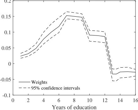
sets of groups are known to the analyst, in other applications they must be estimated. In our supplementary material, we review results from Gentzkow et al. (2011) where these sets are known to the analyst. In Section 6 we review results from Duo (2001) where these sets are not known to the analyst. We propose an estimation procedure and perform a number of robustness checks to assess whether results are sensitive to this rst step estimation procedure. Second, we compute the estimand we suggested in the previous section withG∗ = 1andG∗ = 0
as the treatment and control groups. Third, we compute the estimand we suggested in the previous section with G∗ =−1 and G∗ = 0as the treatment and control groups. Finally, we
compute a weighted average of those two estimands.
In the general case where t > 1, aggregating estimands at dierent dates proves more
di-cult than aggregating estimands from dierent groups. This is because populations switching treatment between dierent dates might overlap. For instance, if a unit goes from non treat-ment to treattreat-ment between period 0 and 1, and from treattreat-ment to non treattreat-ment between period 1 and 2, she both belongs to period 1 and period 2 switchers. A weighted average of, say, our Wald-DID estimands between period 0 and 1 and between period 1 and 2 estimates a weighted average of the LATEs of two potentially overlapping populations. There is therefore no natural way to weight these two estimands to recover the LATE of the union of period 1 and 2 switchers. As shown in the fourth point of the theorem, the aggregated estimand we put forward still satises a nice property: it is equal to the LATE of the union of switchers in the special case where the structure of groups does not change over time and each group experiences a monotonic evolution of its treatment rate over time. When this is the case, pop-ulations switching treatment status at dierent dates cannot overlap, so our weighted average of switchers' LATE across periods is actually the LATE of all switchers.
treatment group and is stable in the control. Finally, when there are more than two groups where the treatment rate is stable over time, our three sets of assumptions become testable. Under each set of assumptions, using any subset ofGs as the control group should yield the
same result.
We now turn to partial identication results when the treatment rate changes in every group. To simplify the exposition, we focus on the case with multiple groups and two periods. Results can easily be extended to accommodate multiple periods.
When the outcome has bounded support[y, y], let, for (d, g)∈ {0,1} × S(G),
Fdg1(y) =M0
1−λgd(1−FYdg1(y))
−M0(1−λgd)1{y < y},
Fdg1(y) =m1
λgdFYdg1(y)
+ (1−m1(λgd))1{y ≥y}.
Then dene
δ−d = max g∈S(G)
Z
ydFdg1(y)−E(Ydg0), δ+d = min g∈S(G)
Z
ydFdg1(y)−E(Ydg0),
WT C− (g) = E(Yg1)−E(Yg0+δ +
Dg0)
E(Dg1)−E(Dg0)
, WT C+ (g) =E(Yg1)−E(Yg0+δ
−
Dg0)
E(Dg1)−E(Dg0)
.
Let alsoFgg0d(y)andFgg0d(y)denote the lower and upper bounds onFY
g1(d)|Sg one can obtain
usingG=g as the treatment group and G=g0 as the control group and applying Theorem
3.3. Finally, let
WCIC− (g) =
Z
max
g0∈S(G)Fgg00(y)−g0min∈S(G)Fgg 01(y)
dy,
WCIC+ (g) =
Z
min
g0∈S(G)Fgg
00(y)− max
g0∈S(G)Fgg01(y)
dy.
Theorem 4.2 Assume that Model (1) and Assumption 1 is satised. Assume also thatGs1=
∅.
1. If Assumption 5 is satised and P(y≤Y(d)≤y) = 1 for d∈ {0,1},
WT C− (g)≤E(Yg1(1)−Yg1(0)|Sg)≤WT C+ (g).
2. If Assumptions 6 and 7 are satised,
WCIC− (g)≤E(Yg1(1)−Yg1(0)|Sg)≤WCIC+ (g).
then select the control group yielding the highest (resp. smallest) lower (resp. upper) bound. Under Assumption 6, one can bound the cdf of Y(1) and Y(0) among switchers in a given
group by using every other group as a potential control group and applying Theorem 3.3. For each value ofy, one can then select the control group yielding the highest (resp. lowest)
lower (resp. upper) bound. One can nally bound switchers LATEs by using integration by parts for Lebesgue-Stieljes integrals. Note that any group can be used to construct bounds for the LATE of switchers in group g, even groups g0 which experienced a larger change of
their treatment rate. Here, we only present partial identication results for treatment eects among switchers of groupg. One can also derive bounds for the entire population of switchers,
by taking a weighted average of these bounds.
4.2 Covariates
We now return to our initial setup with two groups and two periods but consider a framework incorporating covariates. LetX be a vector of covariates. Assume that
Y(d) = hd(Ud, T, X), d∈ S(D),
D = 1{V ≥vGT X}, vG0X =v00X does not depend on G.
(10)
Then we replace Assumptions 1-7 by the following conditions.
Assumption 1X (Conditional time invariance within groups) For d∈ S(D), (Ud, V)⊥⊥T|G, X.
Assumption 2X (Conditional rst stage)
E(D11|X)> E(D10|X), andE(D11|X)−E(D10|X)> E(D01|X)−E(D00|X).
Assumption 3X (Conditional common trends)
E(h0(U0,1, X)−h0(U0,0, X)|G, X) does not depend onG.
Assumption 4X (Conditional common eect of time on both potential outcomes)
E(h1(U1,1, X)−h1(U1,0, X)|G, V ≥v00X, X) =E(h0(U0,1, X)−h0(U0,0, X)|G, V ≥v00X, X).
Assumption 5X (Conditional common trends within treatment status)
E(h0(U0,1, X) −h0(U0,0, X)|G, V < v00X, X) and E(h1(U1,1, X) − h1(U1,0, X)|G, V ≥ v00X, X) do not depend on G.
Assumption 6X (Monotonicity)
Assumption 7X (Data restrictions)
1. S(Ydgt|X = x) = S(Y) = [y, y] with −∞ ≤ y < y ≤ +∞, for (d, g, t, x) ∈ S(D)× S(G)× S(T)× S(X).
2. FYdgt|X=x is strictly increasing on R and continuous on S(Y), for (d, g, t, x) ∈ S(D)× S(G)× S(T)× S(X).
3. S(Xgt) =S(X) for (g, t)∈ S(G)× S(T).
For any random variableR, letDIDR(X) =E(R11|X)−E(R10|X)−(E(R01|X)−E(R00|X)).
We also letδd(x) =E(Yd01|X =x)−E(Yd00|X =x),Qd,x(y) =FY−1
d01|X=x◦FYd00|X=x(y), and
WDID(X) =
DIDY(X)
DIDD(X)
WT C(X) =
E(Y11|X)−E(Y10+δD10(X)|X)
E(D11|X)−E(D10|X)
WCIC(X) =
E(Y11|X)−E(QD10,X(Y10)|X)
E(D11|X)−E(D10|X) .
Finally, letS1={V ∈[v11X, v00X], G= 1}and ∆(X) =E(Y11(1)−Y11(0)|S1, X).
Theorem 4.3 Assume that Model (10) and Assumptions 1X-2X hold, and that for every
d∈ S(D), 0< P(D00=d|X) =P(D01=d|X) almost surely. Then
1. If Assumptions 3X-4X are satised, WDID(X) = ∆(X) and
WDIDX ≡ E[DIDY(X)|G= 1, T = 1]
E[DIDD(X)|G= 1, T = 1]
= ∆.
2. If Assumption 5X is satised, WT C(X) = ∆(X) and
WT CX ≡ E(Y11)−E[E(Y10+D10δ1(X) + (1−D10)δ0(X)|X)|G= 1, T = 1]
E(D11)−E(E(D10|X)|G= 1, T = 1)
= ∆.
3. If Assumptions 6X-7X are satised, WCIC(X) = ∆(X) and
WCICX ≡ E(Y11)−E[E(D10Q1,X(Y10) + (1−D10)Q0,X(Y10)|X)|G= 1, T = 1]
E(D11)−E(E(D10|X)|G= 1, T = 1)
= ∆.
Incorporating covariates into the analysis has two advantages. First, it allows us to weaken our identifying assumptions. For instance, when the distribution of someX evolves over time
in the control or in the treatment group, Assumption 1X is more plausible than Assumption 1: if the distribution ofX is not stable over time and X is correlated with (Ud, V), then the
the control group, the evolution of the treatment rate is entirely driven by a change in the distribution of X. If that is the case, one can use the previous theorem to point identify
treatment eects among switchers, while our theorems without covariates only yield bounds. When P(D00 = d|X) 6= P(D01 = d|X), one can derive bounds for ∆(X) and then for ∆.
These bounds could be tighter than the unconditional ones if changes in the distribution of
X drive most of the evolution of the treatment rate in the control group.
4.3 Non-binary, ordered treatment
Finally, we consider the case where the treatment is not binary but takes a nite number of values: D ∈ {0,1, ..., d} and is ordered. One prominent example is education, considered in
the application below. We extend our model to this case as follows:
Y(d) = hd(Ud, T), d∈ {0, ..., d},
D = Pd
d=11{V ≥vGTd }, −∞=vgt0 < vgt1... < vgtd+1 = +∞((g, t)∈ {0,1}2).
(11)
Assumption 4O (Common average eect of time on all potential outcomes) For d∈ {0, ..., d},
E(hd(Ud,1)−hd(Ud,0)|G, V ∈[vGd0, vGd+10 )) =E(h0(U0,1)−h0(U0,0)|G, V ∈[v
d
G0, vGd+10 )).
Assumption 5O (Common trends within treatment status at date 0)
For every d∈ S(D), E(hd(Ud,1)−hd(Ud,0)|G, V ∈[vGd0, vdG+10 ))does not depend on G.
Model (11) and Assumptions 4O-5O generalize respectively Model (1) and Assumptions 4-5 to situations where the treatment is non-binary and ordered . Let&denote stochastic dominance
between two random variables, while ∼denotes equality in distribution.
Theorem 4.4 Assume that Equation (11) and Assumptions 1-2 are satised, thatD01∼D00,
and that D11&D10. Let wd= P(DE11(D≥11d))−−EP((DD1010≥)d).
1. If Assumptions 3 and 4O are satised,
WDID= d
X
d=1
E(Y11(d)−Y11(d−1)|V ∈[vd11, vd10))wd.
2. If Assumption 5O is satised,
WT C = d
X
d=1