On using surrogates with genetic programming

http://wrap.warwick.ac.uk

Original citation:

Hildebrandt, Torsten and Branke, Juergen (2014) On using surrogates with genetic

programming. Working Paper. Coventry, UK: University of Warwick, WBS.

Permanent WRAP url:

http://wrap.warwick.ac.uk/60025

Copyright and reuse:

The Warwick Research Archive Portal (WRAP) makes this work by researchers of the

University of Warwick available open access under the following conditions. Copyright ©

and all moral rights to the version of the paper presented here belong to the individual

author(s) and/or other copyright owners. To the extent reasonable and practicable the

material made available in WRAP has been checked for eligibility before being made

available.

Copies of full items can be used for personal research or study, educational, or

not-for-profit purposes without prior permission or charge. Provided that the authors, title and

full bibliographic details are credited, a hyperlink and/or URL is given for the original

metadata page and the content is not changed in any way.

A note on versions:

The version presented here is a working paper or pre-print that may be later published

elsewhere. If a published version is known of, the above WRAP url will contain details

on finding it.

On Using Surrogates

with Genetic Programming

Torsten Hildebrandt

Bremer Institut f ¨ur Produktion und Logistik - BIBA an der Universit¨at Bremen, Bremen, Germany

J ¨urgen Branke

Warwick Business School, University of Warwick, CV4 7AL Coventry, UK

Abstract

One way to accelerate evolutionary algorithms with expensive fitness evaluations is to combine them with surrogate models. Surrogate models are efficiently computable ap-proximations of the fitness function, derived by means of statistical or machine learn-ing techniques from samples of fully evaluated solutions. But these models usually require a numerical representation, and therefore can not be used with the tree repre-sentation of Genetic Programming (GP). In this paper, we present a new way to use surrogate models with GP. Rather than using the genotype directly as input to the sur-rogate model, we propose using a phenotypic characterization. This phenotypic char-acterization can be computed efficiently and allows us to define approximate measures of equivalence and similarity. Using a stochastic, dynamic job shop scenario as an ex-ample of simulation-based GP with an expensive fitness evaluation, we show how these ideas can be used to construct surrogate models and improve the convergence speed and solution quality of GP.

Keywords

Genetic Programming, surrogates, phenotypic characterization.

1

Introduction

For many practical applications, the most time consuming part of Evolutionary Algo-rithms (EAs) is the fitness evaluation. For example in engineering design, evaluating a single solution may take several hours. In order to speed up the execution of EAs with expensive fitness evaluations, integrating surrogate functions attracted much re-search (Jin, 2005, 2011). The basic idea here is to minimize the number of expensive fitness evaluations by replacing them with a computationally cheaper function as far as possible. To learn such surrogate functions1 _{from a sample of fully evaluated}

so-lutions, various statistical or machine learning techniques can be used. These models usually assume a numerical representation of the solutions, as they require a measure of ”distance” or ”similarity” between solutions. Because the genotype in GP is a tree structure, it is not straightforward to use surrogate models with GP.

In this paper, we present an approach that allows surrogate models to be used with GP. Rather than trying to learn an approximate function that maps the genotype (i.e., a GP tree) into the fitness, we introduce the concept of a phenotypic characterization of a solution. This phenotypic characterization tries to capture thebehaviorof the phenotype encoded in the GP tree, and represents it as a vector of numerical values, which then allows calculating distances among individuals as required by the surrogate models. We show how this idea can be used to remove duplicates and reduce the number of necessary expensive fitness evaluations, thus generating better results more quickly. Our approach thus makes GP more efficient when applied to problems with expensive fitness evaluation, and opens up the possibility of using GP also on problems which previously have been computationally too demanding.

The exact phenotypic characterization is problem specific. However, the general idea is generic and should be applicable across application domains. To demonstrate the usefulness of our proposal, we use the task of evolving dispatching rules for shop scheduling as an example of GP with expensive fitness evaluation.

This paper is structured as follows. After reviewing related work in Section 2 we describe our application area in Section 3. In Section 4, we introduce the concept of a phenotypic characterization, present such a characterization for dispatching rules, and describe its use to establish (approximate) phenotypic equivalence and similarity be-tween GP trees encoding dispatching rules. Section 5 presents our experimental setup. The results presented in Section 6 demonstrate the usefulness of the introduced con-cepts to improve the convergence of GP by

1. detecting and suppressing phenotypic duplicates

2. supplementing GP with a surrogate function that uses approximate phenotypic similarity between individuals.

We analyze what data to base the phenotypic characterization on, and compare the performance of agenotypicsimilarity measure for GP trees with thephenotypicsimilarity introduced in this paper. We conclude with a summary and outlook towards future work.

2

Related Work

The use of approximate but cheap to evaluate learned surrogate models to speed up evolutionary algorithms on problems with expensive fitness functions has been pro-posed many years ago (e.g., Rattle (1998)) and meanwhile is an established research area. In the following, we briefly discuss some of the most relevant papers. For a more comprehensive review, the interested reader is referred to, e.g., Jin (2005, 2011); Shi and Rasheed (2010); Jin and Branke (2005).

data used to learn the surrogate model can come from an experimental design con-ducted before the EA, but usually is learned and adopted online during the run (Jin, 2005, 2011; Jin and Branke, 2005).

Surrogate models can be used to support EAs in several ways. Most often, all in-dividuals are evaluated with the surrogate model, and this information is used to pre-select the most promising individuals that are then evaluated with the expensive fit-ness function (Jin et al., 2002). That way, individuals classified as poor by the surrogate model can be quickly discarded, while the better individuals are fully evaluated to al-low an accurate ranking. Furthermore, the full evaluation of these individuals are used to further refine the surrogate model particularly in the most promising areas. Others have proposed to alternate between generations that are evaluated with the surrogate model and generations that are evaluated using the expensive fitness function (Rattle, 1998; Jin et al., 2002), to use surrogate models for supporting local search (Lim et al., 2010), or for pre-selection amongst individuals generated by a genetic operator (Em-merich et al., 2002).

However, so far, successful use of surrogates to speed up EAs has been restricted to fixed-length representations for which it was easy to define a distance metric (e.g., bit-strings or vector of real values). GP, on the other hand, usually uses a tree repre-sentation of variable length. Machine learning or statistical techniques can not be used directly to work with such genotypes or phenotypes, which probably is the reason why, to the best of our knowledge, no other work using surrogate functions with GP is reported in the literature. In this paper we overcome these difficulties by using an (ap-proximate) phenotypic characterization of the individual. As it is a vector consisting of integer values, we can then apply standard techniques from the surrogate literature to estimate the fitness value of a GP individual without performing an expensive fitness evaluation.

A few papers in the GP area area related to our idea of phenotypic representation in the sense that they propose considering the behavior of solutions in GP rather than just the genotype. So far, however, this idea has not been used to construct surrogate models.

solution quality of standard GP. Here we further analyze this approach and extend it to create surrogate functions to improve the convergence of GP. As an extreme op-tion to diversity preservaop-tion, Lehman and Stanley (2010) propose focusing on novelty instead of the objective function value when selecting individuals, and again use the phenotypic behavior to determine novelty.

In Uy et al. (2011) the authors use the above mentioned Sampling Semantic Dis-tance in order to define tree similarity and use it in an improved crossover operator to enforce crossover between subtrees in a certain similarity range. They report improved results on a number of symbolic regression problems.

Finally, Ashlock and Lee (2013) recently proposed the concept of ”agent-case em-bedding” that is closely related to our concept of phenotypic characterization and is used for analyzing evolved systems.

3

Evolving Dispatching Rules

The application we consider in this paper as an example is the problem of evolving dispatching rules for dynamic job shop scheduling problems. A dispatching rule is a simple heuristic that computes a priority value for a job from its attributes (Haupt, 1989; Blackstone et al., 1982; Holthaus and Rajendran, 1997; Rajendran and Holthaus, 1999). Whenever a machine becomes idle and has waiting operations in its queue, the job with the highest priority value is chosen to be processed next. Benefits of dispatching rules include their simple and intuitive nature, their ease of implementation within practical settings, and their flexibility to incorporate domain knowledge and expertise. They are very well suited for online scheduling, as they automatically take into account the latest information available. All these factors have led to their frequent use in various industries including semiconductor manufacturing (Pfund et al., 2006).

Usually, dispatching rules are designed by experts in a tedious trial-and-error pro-cess, with candidate rules being tested in a simulation environment, modified and re-tested until they fulfill the requirements for actual implementation in practice (Geiger et al., 2006). In recent years, several authors have suggested to automatically design suitable dispatching rules by means of EAs, see for example Geiger et al. (2006); Di-mopoulos and Zalzala (2001); Pickardt et al. (2013, 2010); Nguyen et al. (2013b,a). Most of these approaches use Genetic Programming (Koza, 1992; Poli et al., 2008) and can be classified as applications of hyper-heuristic search (Burke et al., 2009, 2010). As such their search space is the space of heuristics instead of a concrete solution of a problem instance.

In terms of the set of terminals and non-terminals, finding a dispatching rule is similar to symbolic regression, a standard GP benchmark problem. A GP individual encodes an arithmetic expression, a function of several variables. In case of a dispatch-ing rule, the GP individual encodes a functionp : Ra → Rmapping a vector of a

attributes describing a job, machine, or the whole system to a priority value. Fitness evaluation is far more complex, however, and usually involves running multiple repli-cations of a stochastic, dynamic shop floor simulation. The time required for just a single fitness evaluation therefore by far exceeds the computational time required by the core GP algorithm.

P i i

‐

Priority

0

+

+

NPT

+

+

WINQ NPT

PT PT

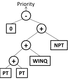
Figure 1: GP tree representation of the Holthaus rule -(2PT + WINQ + NPT) (Holthaus and Rajendran, 2000), where PT, WINQ and NPT denote processing time, work in next queue, and processing time at the next machine, respectively.

for various scheduling problems ranging from single machine problems (e.g., Geiger et al. (2006)), classic static job shop scheduling problems (Nguyen et al., 2013b), to dy-namic job shop scheduling problems (e.g., Hildebrandt et al. (2010)). Recently also dispatching rules for a complex dynamic scenario from semiconductor manufacturing were evolved using GP (Pickardt et al. (2013, 2010)). This scenario consists of 36 ma-chines, sequence dependent setup times, parallel mama-chines, batch machines and reen-trant process flows with jobs consisting of up to 92 operations. Rules developed by GP for this scenario clearly outperformed standard dispatching rules from the literature. To use GP in such a setting is computationally very demanding. The method presented in this paper is one step towards an increased scalability of GP to even larger practical scenarios requiring even longer simulation times.

In terms of the scheduling scenario considered we take one step back in this paper by considering a dynamic job shop scenario with 10 machines proposed by Rajendran and Holthaus (1999) and described in more detail in Section 5.1. Using this scenario (taking about 0.6s per fitness evaluation) seems complex enough to justify the use of a surrogate model, but still keeps computational times low enough to be able to investi-gate a variety of different parameter settings and perform each experiment a number of times to obtain statistically valid results on mean performance, etc.

4

Approach

4.1 Overview

Before presenting in detail how to compute the phenotypic characterization and how to use it to define (approximate) equivalence and similarity, we show in this section how they are embedded in the overall solution procedure. Figure 2 depicts the general outline of an optimization run. The general procedure is based on a generational re-production scheme, as used for instance in conventional GP. In Figure 2 standard steps are shown as white boxes, additional steps related to the use of surrogates and detec-tion/removal of phenotypic duplicates are shown as grey boxes. Each iteration of the main loop (steps 3 to 9) constitutes one generation.

We start with a populationP of rules/individuals (step 1). These initial rules are usually randomly generated using some initialization procedure. In step 2 we remove duplicate rules using the procedure decribed in Section 4.3 and replace them with ad-ditional random rules until our population consists of the required number of different rules.

All candidate rules inPare subsequently fully evaluated in a simulation in step 3. As already mentioned, this is by far the most time-consuming step in the overall pro-cedure. Once real fitness values are known, we check whether the optimization run should be terminated or continue with another iteration. If we decide to terminate, the best rule found so far is reported as the result of the optimization run. Otherwise, we update our surrogate model to incorporate the new fitness values of all individuals in

P(step 4).

In the next step (step 5), conventional GP operators (see Koza (1992); Poli et al. (2008)) for selection, mutation, and crossover are used to produce a new, intermediate populationPimdtaking into account all individuals inP and their fitness values. Tree

mutation works by replacing a node of the tree by a new, randomly created subtree. Tree crossover takes two parent trees and produces two offspring trees by exchanging a randomly selected sub-tree between the two parents.

Duplicates inP_imd are subsequently removed in step 6 and replaced with addi-tional individuals generated fromP in the same way as in step 5. At this stage we have a set of individuals which produce with a very high probability distinct (as will be examined in Figure 4a) fitness values.

In conventional GP, bothP andPimdcontain the same number of individuals. As

we want to use the surrogate model to select the most promising individuals later on, we have to create more rules in this step, i.e.,|Pimd|= n|P|withn > 1. In the

exper-imental section of this paper, we investigate different values ofn. Settingntoo low will result in only minor improvements over standard GP, setting it too large may have negative consequences on convergence, because inaccuracies of the surrogate function may have a lot of impact and misguide the GP.

1. Generate Random Rule Population P

3. Full Fitness Evaluations

5. Produce Offspring from P in Pimd

4. Update Surrogate Model 7. Compute Phenotypic Charact.

9. Fill P with Best Rules from Pimd

8. Estimate Fitness using Surrogate Budget left?

2. Remove Duplicates from P

6. Remove Duplicates from Pimd

[no]

[yes] Best Rule of Run

Figure 2: General solution approach. Components of standard GP are shown as white boxes. Additional steps related to the use of surrogates and detection/removal of phe-notypic duplicates are shown as grey boxes.

decision situation

attribute sets

s1 s2 s3

ranking by reference rule

ranking by other rule

decision vectord

1

1 37 46 158 12 21 2

2 23 17 1 2 2 2 8 9 3 3 1 3

2 8 9 3 3 1 3

2 6 4 6 1 3

… … … … …

k 4 8 6 1 1 1

k 7 3 9 2 2

(a)

d d d fit

… …

…

d1 d2 dkfitness rule1: 2 3 1 1456

… … rule2: 1 2_{… …} … 2 1123_… rulem: 1 3 … 1 1293

(b)

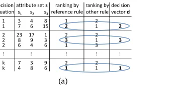
Figure 3: Phenotypic charaterization of dispatching rules. (a) creation of a decision vector for a certain rule given a set of kdecision situations. (b) database ofmrules, their decision vectors and fitness values.

As a next step (step 9), estimated fitnesses are used to select the most promising candidates to form a new populationP for the next iteration. Step 3 starts a new iter-ation of the main optimiziter-ation loop again fully evaluating each individual inP using the expensive fitness function.

4.2 Phenotypic Characterization of Dispatching Rules

The key to using a surrogate model with GP is to come up with a meaningful dis-tance metric. Because this is difficult on the genotype level (trees), in the following we propose a phenotypic characterization. The phenotypic characterization looks at the

behaviorof the evolved rules, rather than their syntactic description. This is naturally

problem-dependent. In the following, we develop a phenotypic characterization for evolving dispatching rules in job shop scheduling. However, similar phenotypic char-acterizations can also be developed for other problem domains, and Ashlock and Lee (2013) may serve as additional inspiration.

is free and there are jobs waiting, the rule is used to sequence all jobs by their priority, and the job with highest priority is processed next. The key characteristic of dispatching rules is not the functional values they compute, but only to which of a set of jobs they assign the highest priority.

Consequently, the phenotypic characterization for dispatching rules we propose here is a decision vector, a record of all the decisions a dispatching rule takes in a com-parably small number ofkdecision situations, as outlined in Figure 3. These decision situations could be sampled from an actual simulation run, or simply be created ran-domly. This later aspect is analyzed in more depth in Section 6.2.

The rule to be characterized is used to rank all jobs in each decision situation to find out which job is given the highest priority in each situation (rank 1). A certain fixed reference rule is also used to rank jobs in each decision situation. The decision vectordto characterize a ruleRconsists of, for each decision situation, the rank the reference rule assigned to the job receiving top priority by ruleR. Consider the example in Figure 3(a). In the first decision situation, there are two jobs to choose from. Rule

Rgave the highest priority (rank 1) to the second job. This job was ranked second by the reference rule, sod1 = 2. Similarly, in the second decision situation, ruleRgives the first rank to the second of three jobs, which has been ranked third by the reference rule, thusd2 = 3. For decision situationk, ruleRprioritizes the second job, which is in concordance with the reference rule, and thusdk = 1. In summary,dconsists ofk

integer values expressing the similarity ofRto the reference rule. A rule leading to the same decisions as the reference rule has all elements of the vector set to 1. A rule which always selects the job that has the lowest priority according to the reference rule has all elements set to the highest possible values, i.e., the number of jobs in the corresponding decision situation (note that this means the maximal error a rule can make depends on the number of jobs in a particular decision situation, and may be different for different situations).

This definition completely abstracts from the actual priority values produced by a rule. Therefore also syntactically quite distinct rules (such as ”1/PT” vs. ”−PT” as two possibilities to express the well-known rule ”shortest processing time first”) would be recognized as being equivalent.

Obviously, the computational effort to compute the phenotypic characterization is much less than running a full, expensive fitness-evaluation, which would involve tens of thousands of such decisions.

4.3 Approximate Phenotypic Equivalence and Similarity

We use the phenotypic characterization to build a surrogate function that can help us estimate the fitness value of new individuals at much lower computational cost than the full evaluation via simulation. The surrogate function takes the phenotypic charac-terization (i.e., the decision vectordin our case) as input, and provides the estimated fitness as output. Constructing the surrogate function from a given set of input-output pairs (see Figure 3b) is a typical machine learning or regression task, and standard techniques such as Neural Networks, Gaussian Processes or Regression Tress could be used.

individuals in the database are computed using the Euclidean distance between phe-notypic characterizations. The fitness of the most similar individual is returned as the fitness estimate for the new individual.

To detect and remove phenotypically identical rules we could use identical de-cision vectors as a criterion. For this task an even simpler criterion turned out to be sufficient, however: We only consider a single decision situation consisting of 100 jobs. Values of the attribute set are created randomly within typical value ranges but not taking into account any dependencies or correlations between the attributes. Two rules are considered identical, if they produce the same rank vector for these 100 jobs.

5

Experimental Setup

5.1 Shop Floor Scenario

Our computational experiments use the dynamic job shop-scenarios from Rajendran and Holthaus (1999) and try to find good dispatching rules for these scenarios auto-matically. In total there are 10 machines on the shop floor, each job entering the system is assigned a random routing, i.e., machine visitation order is random with no machine being revisited. Processing times are drawn from a uniform discrete distribution rang-ing from 1 to 49 minutes. Job arrival is a Poisson process, i.e., inter-arrival times are exponentially distributed. The mean of this distribution is chosen to reach a desired utilization level on all machines. All experiments in this paper use a (mean) utilization of 95 %. These scenarios were also used to evolve dispatching rules in Branke et al. (2013) and Hildebrandt et al. (2010).

Following the procedure from Rajendran and Holthaus (1999), we start with an empty shop and simulate the system until the first 2500 jobs have been completed. Data on the first 500 jobs is discarded to focus on the shop’s steady state-behavior. The objective function is to minimize the mean flowtime, i.e., the arithmetic mean of the flowtimes of jobs 501 to 2500: FT= ₂₀₀₀1 P2500_j=501(Cj−rj), whereCjis the completion

time of a jobjandrjis its arrival time.

Because the simulation is stochastic, also the calculated flowtime is a stochastic variable. To reduce the impact of stochasticity, we replicate each simulation 10 times for each fitness evaluation and use the average performance for optimization. Fur-thermore, we use the same 10 random number seeds to evaluate all solutions during optimization (common random numbers, (Law, 2007)). All results reported in this pa-per are based on evaluating the resulting rules on adifferentset of 100 independent test runs. The simulation has been implemented in Java, and is publicly available (Hilde-brandt, 2012).

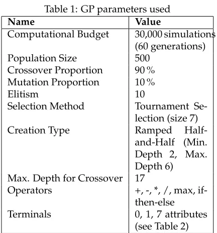
Table 1: GP parameters used

Name Value

Computational Budget 30,000 simulations (60 generations) Population Size 500

Crossover Proportion 90 % Mutation Proportion 10 %

Elitism 10

Selection Method Tournament Se-lection (size 7) Creation Type Ramped

Half-and-Half (Min. Depth 2, Max. Depth 6)

Max. Depth for Crossover 17

Operators +, -, *, /, max, if-then-else Terminals 0, 1, 7 attributes

(see Table 2)

Table 2: Information available to be used in dispatching rules (terminal set).

Attribute Norm.

Range

Explanation

PT [1, 47] Processing Time of Current Operation

NPT [0, 47] Next Processing Time, i.e., Processing Time of Next Operation

WINQ [0, 410] Work In Next Queue, i.e., Sum of Processing Times of All Jobs at the Next Machine

RemProcTime [1, 264] Remaining Processing Time, i.e., Sum of Pro-cessing Times of All Unfinished Operations OpsLeft [1, 10] Operations Left, i.e., Number of all Unfinished

Operations

TimeInQueue [0, 1500] Time Since Arrival in Current Queue TimeInSystem [0, 2770] Time Since Arrival in System

5.2 Genetic Programming

For our experiments we used the Genetic Programming implementation of the Evo-lutionary Computation in Java (ECJ)-framework2_{. Details of the parameters used are}

shown in Tables 1 and 2. This choice of parameters and terminal set resembles the best settings identified for the tree representation in Branke et al. (2013), where we could also identify normalization of input attributes in a common value range of [0, 2] to improve GP performance. We therefore also use these settings for the experiments re-ported in this paper. Unless mentioned otherwise, convergence curves in this paper are based on 100 independent runs.

5.3 Surrogate Function

We use a Nearest Neighbor Learner as a modeling technique. The Nearest Neighbor surrogate model uses the full fitness evaluations of the last two generations, i.e., 1000 fully evaluated individuals are used to predict the fitness of new individuals. To pre-dict the fitness of a new individual, the distances to all the 1000 individuals in the database are computed using the genotypic (syntactic) or phenotypic distance mea-sures as described below. The fitness of the most similar individual is returned as the fitness estimate for the new individual.

As mentioned in the previous sections, it is very difficult to use surrogate functions for GP’s tree representation, as popular surrogate modeling techniques such as Neural Networks or Polynomial Regression can only learn functional relationships between real- or integer-valued vectors and a fitness value. In order to use a Nearest Neighbor learner, however, we only have to specify a distance measure between solutions. We can therefore use this learning method to compare surrogates based not only on the phenotypic characterization proposed above in Section 4.2, but also based on a geno-typic distance metric from the literature.

More formally, for our phenotypic characterization, the distanceD between two decision vectorsd˜anddˆwithndimensions is computed as

D( ˜d,dˆ) =

v u u t

n

X

i=1

˜

di−dˆi

2

.

Genotypic similarity between expression trees is computed using the Structural Hamming Distance (SHD), which was presented in Moraglio and Poli (2005) to create an improved crossover operator.

SHD(T1, T2) =     

   

1 ifarity(p)6=arity(q)

hd(p, q) ifarity(p) =arity(q) = 0

1

m+1(hd(p, q) + Pm

i=1SHD(si, ti))

ifarity(p) =arity(q) =m

It defines a syntactic distance measure between trees ranging from 0 (trees are equal) to a maximum distance of 1. In this formulaT1 andT2 are trees, pandqare their root nodes andsias well astidenote theith subtree ofpandqrespectively. The

utility functionarity(p)computes the number of a node’s subtrees. hd(p, q)computes the Hamming distance betweenpandq, which is 0 ifp=q, i.e.,pandqrepresent the same type of terminal or non-terminal node, or 1 otherwise.

6

Results

6.1 Duplicate Detection and Removal

equiva-Generation Fr action Unique 0.0 0.2 0.4 0.6 0.8 1.0

0 10 20 30 40 50

(a)

Generation

Additionally Created Individuals ₀

100 200 300 400 500 ● ● ● ● ● ●_{● ● ● ● ● ● ● ● ● ● ● ● ● ● ● ● ● ●}● ● ● ● ● ● ● ●● ● ● ● ● ●● ● ● ●● ● ● ●● ● ●● ● ● ● ● ● ●● ● ● ●

0 10 20 30 40 50

(b)

Objective Function Evaluations

Mean Flo wtime 0.92 0.94 0.96 0.98 1.00 1.02 1.04

103 ₁₀3.5 ₁₀4

(c)

Objective Function Evaluations

Standard Error 0.0010 0.0015 0.0020 0.0025 0.0030 0.0035

103 ₁₀3.5 ₁₀4

(d)

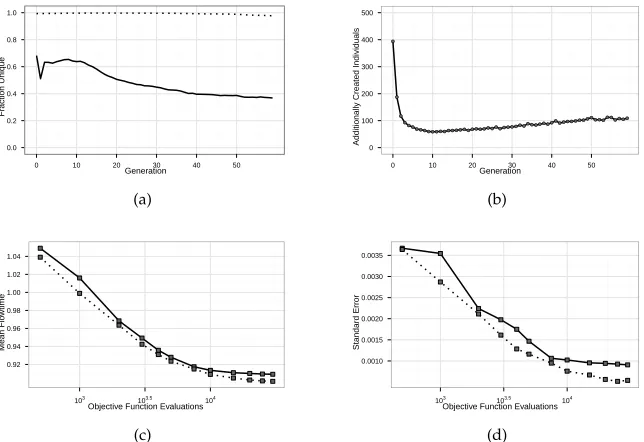
Figure 4: Figure 4a shows the fraction of individuals with unique fitness values for Standard GP (solid line) and when using (approximate) duplicate detection (dotted line). The number of additional individuals required to increase diversity is shown in Figure 4b (population size is 500). Mean performance (4c) and standard error (4d) of GP runs with (dotted lines) and without (solid lines) suppression of duplicates based on (approximate) phenotypic equivalence. Performances are relative to the mean flowtime achieved by the Holthaus rule and averaged over 100 runs.

lence we eliminate all duplicate rules in a population before running any simulations to assess rule performances. These rules are replaced with new rules either created ran-domly (initial population), or, later on in a GP run, by using the mutation/crossover operators.

As shown by the dotted line in Figure 4a, this duplicate avoidance scheme is quite successful at maintaining a high level of diversity (measured in the number of indi-viduals with distinct fitness values). Standard GP (solid line) starts with a consider-ably lower diversity, and depicts a further decreasing diversity after generation 13. The number of individuals created additionally to replace duplicates is shown in Fig-ure 4b. Interestingly, especially for the initial population and the first few generations, the number of additionally created individuals is rather high, before dropping to a level of around 60 additional individuals per generation. From around generation 10 this number is increasing again with a linear trend. This is consistent with the behavior of standard GP: from about generation 10-13 it seems to become increasingly difficult for GP to find new, fitness-distinct individuals, therefore more individuals have to be created to compensate.

be beneficial for the evolutionary process. However, a look at the convergence lines in Figure 4c shows a clear advantage of removing fitness duplicates: Both, convergence speed and final solution quality, improve. Also the standard error and therefore stan-dard deviation of run performance decreases (see Figure 4d), leading to more reliable optimization results. We can therefore conclude that at least in the considered appli-cation, removing phenotypically equivalent rules allows finding better solutions more quickly.

Summarizing, without using any additional expensive simulation runs, and with very low additional computational cost, we can almost entirely remove fitness dupli-cates, allowing a faster convergence to a better performance level.

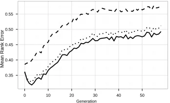
6.2 Choosing a Set of Decision Situations

The phenotypic characterization of a dispatching rule (Section 4.2) depends on the rule’s behaviour on a set of decision situations. Obviously, the set of decision situa-tions selected has an impact on the quality of the resulting surrogate model, and the question arises how to create this set. For example, it could be created randomly, or by sampling real situations encountered in a simulation. To examine the influence of different ways to chose the set of decision situations, we analyze the ranking perfor-mance of the resulting surrogate models, based on the individuals of 30 GP runs (with suppression of duplicates but not using a surrogate function). Data of all individu-als created is recorded and used to learn surrogate models from three different sets of decision situations; in all cases a set consists of 100 situations:

• Random: Decision situations are created randomly containing between 2 and 20

”jobs”. Similar to the technique to detect duplicates for each of these ”jobs” ran-dom values are created for each of the attributes within the ranges listed in Table 2 using a uniform continuous distribution. This approach assumes all attributes to be independent. It is pretty simple as it only depends on knowing typical value ranges of the attributes, no additional simulation runs are required.

• Reference rule: Decision situations are sampled from preliminary simulation runs

using the Holthaus rule. From all real decision situations encountered in such a simulation, a sub-set of 100 situations is sampled.

• Optimized rule: As optimization progresses and decisions of optimized rules get

increasingly different, situation characteristics might change. Thus, it might be ad-vantageous to change decision situations during an optimization run. To quantify this effect we used the best rules from 30 GP runs to sample decision situations, anticipating the situations encountered by rules at the end of an optimization run. Obviously, this would not be feasible in practice, but may serve as an indication for the performance when the set of decision situations is adapted dynamically to always reflect the best solution found so far.

Generation

Mean Rank Error

0.35 0.40 0.45 0.50 0.55

0 10 20 30 40 50

Figure 5: Choice of decision situations for phenotypic characterization: dashed line: random decision situations; dotted line: decision situations sampled with reference rule; solid line: decision situations sampled with optimized rules. All lines show the mean rank error, normalized to the expected error of random selection.

with Euclidean distance as a similarity measure, we created surrogate models using the phenotypic characterization based on each set of decision situations.

The quality of a surrogate model is judged as its ability to produce the same rank-ing that would result from the expensive fitness evaluations, which seemed the most relevant aspect given that we are using a rank-based selection scheme. We measure this by looking at the mean rank error of the predictions, normalized to the expected rank error of a random ordering of the individuals. The best possible error of 0 would mean the surrogate can produce a perfect ranking. In this case, the computationally expensive simulation runs could be replaced with the surrogate without any impact on GP performance. In the other extreme, a model with quality 1 is not better than using a random permutation of individuals. For a more detailed discussion of appropriate measures of surrogate quality see Jin et al. (2003).

Results in Figure 5 show the surrogate’s quality when using the individuals (and their fitness) from a certain generation as training data to predict the performance of the individuals of the next generation. For each graph in Figure 5, we tested each of the 30 different sets of decision situations with each of the 30 recorded runs.

Generation

Mean Rank Error

0.4 0.5 0.6 0.7 0.8

0 10 20 30 40 50

Figure 6: Genotypic vs. phenotypic surrogate. The lines show the (normalized) mean rank error using SHD as a genotypic similarity measure (dash-dot line) vs. approximate phenotypic similarity (dashed line: random decision situations; dotted line: decision situations sampled with reference rule).

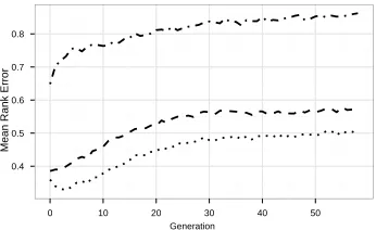
6.3 Phenotypic vs. Genotypic Surrogate

The Nearest Neighbor surrogate model used in this paper only requires a distance met-ric to be applied. In order to demonstrate that the proposed phenotypic characteriza-tion allows for much more meaningful distance metric than genotypic distances, in this section we compare the surrogate quality based on our phenotypic characterization with a surrogate model using the genotypic SHD distance measure (Moraglio and Poli, 2005), following the same experimental setup as described in the previous section.

Results are shown in Figure 6 comparing surrogate quality using phenotypic sim-ilarity from the previous section (based on random decision situations—dashed line; based on reference rule—dotted line) with genotypic similarity (dash-dot line). Results clearly show a much better performance of the surrogate model based on our pheno-typic characterization. Even using random decision situations leads to much better results than the surrogate based on SHD distances. Especially in later generations, the ranking produced by the surrogate model based on SHD distances is only slightly bet-ter than simply creating a random permutation of individuals.

6.4 Phenotypic Surrogate for GP

● ● ● ● ● ● ● _● ● ● ● ● 0.90 0.95 1.00 1.05 1000 10000

Fitness Function Evaluations

Mean Flo

wtime

(a) Mean performances.

● ● ●● ● ● ● ● ● ● ● 0 20 40 60 80

0 10000 20000 30000

Standard GP Budget

Budget Sa

v

ed [%]

(b) Budget saved to reach performance of Standard GP.

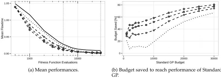
Figure 7: Comparison of Standard GP (solid line), GP with duplicate suppression (i.e.,

n=1; dotted line), and surrogate-supported GP runs (dashed lines). Indicated by the shapes of the dashed lines we investigated three different settings for the number of preselection individuals (n=2: circles;n=5: squares;n=10: diamonds).

Results are given in Figure 7a. The solid and dotted lines show the results of Stan-dard GP and when using duplicate removal (as already presented in Figure 4c). Dashed lines show the convergence lines with surrogates. Different settings ofnare indicated by different shapes to mark data points (circle, square, diamond: n = 2,5,10). As can be seen, using the surrogate model results in faster convergence. Concerning the right size of the intermediate population there is a benefit of using larger values ofn. Increasing n shows decreasing returns, however. The value of the surrogate model therefore seems limited, and for largernthe computational effort to create and evalu-ate (using the surrogevalu-ate) additional individuals would only lead to marginally faster convergence.

These result are presented in a slightly different form in Figure 7b graphically showing the percentage of fitness evaluations saved while still achieving the perfor-mance of standard GP. Data for this graph was obtained by moving a horizontal line in Figure 7a along the solid line, i.e., the convergence curve of standard GP. As an exam-ple, after 5,000 fitness evaluations (dotted vertical line next to the center of Figure 7a) standard GP achieves a performance of about 0.93. The same performance levels are achieved by the other variants considerably earlier, resulting in the saved budget val-ues for a standard GP budget of 5,000 as shown in Figure 7b. The final performance level of standard GP after 30,000 fitness evaluations is reached by the surrogate-assisted variants much earlier, resulting in savings of up to 80% of the fitness evaluations. Al-ready GP with removal of duplicates reaches a very good performance level much more quickly. However, there is a clear additional benefit of using the surrogate model.

● ● ● ● ● ● ●

●● ● ● ●

●● ●

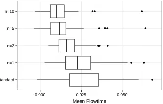
standard n=1 n=2 n=5 n=10

0.900 0.925 0.950

Mean Flowtime

(a) Run performances after 5,000 fitness evaluations. (b) Performance differences after 5,000 fit-ness evaluations.

●● ● ● ● ●

●

● ● ●

●●●

● ●

● ● ● ●

standard n=1 n=2 n=5 n=10

0.900 0.925 0.950

Mean Flowtime

(c) Run performances after 30,000 fitness evaluations.

n=1 n=2 n=5 n=10

standard 10.2 (++) 10.7 (++) 8.5 (++) 7.1 (++)

n=1 0.5 (o) ‐1.7 (o) ‐3.1 (+)

n=2 ‐2.2 (o) ‐3.6 (++)

n=5 ‐1.4 (o)

(d) Performance differences after 30,000 fit-ness evaluations.

For example, a difference of 10.2 between ”standard” and ”n=1” means a worse perfor-mance of Standard GP in comparison with the setting ofn=1 by 10.2 minutes of flow time on average. Indications of statistical significance of these differences are shown in brackets. They are based on a non-parametric, paired Wilcoxon signed-rank test.

As can be seen in Figure 8d, all settings forndominate the performance of Stan-dard GP. Comparingn= 1withn= 2, i.e., using removal of duplicates and duplicate removal with pre-selection withn= 2, both lead to about the same performance level (slightly better result ofn= 2is not significant). Given the faster convergence,n= 2 is a much better choice. Increasingnfurther accelerates convergence, but performance for large budgets stagnates, performance ofn = 10is significantly worse than that of

n= 1orn= 2. At an intermediate budget of 5,000 fitness evaluations (shown in Fig-ures 8a and 8b) a high setting ofnis still beneficial, however increasingnfrom 5 to 10 results only in a non-significant improvement of performance.

We explain this by the search bias introduced with the surrogate model. As long as there only is a modest influence of the model, convergence is not affected. If the model’s influence is high due to a largen, errors introduced by the model can lead to premature convergence in sub-optimal parts of the search space. Furthermore, given the results of Section 6.3, it seems to be more easy to differentiate between good and bad rules in the first few generations when individuals in the population are very dissimilar with a large variance of fitness values.

When optimizing with expensive fitness functions, detailed convergence lines as shown in Figure 7 will generally not be known in advance. Therefore, given a certain computational budget, a robust setting is required, which combines fast convergence with a good convergence level and low computational overhead. Given these require-ments, using the phenotypic surrogate with a moderate setting ofn = 2. . .3 seems to be a good compromise to achieve faster convergence without sacrificing the final convergence level achievable.

6.5 Runtime Considerations

Using Surrogate-Assisted GP as presented in this paper requires additional computa-tional time compared to Standard GP. For each generation, i.e., iteration of the main loop of Figure 2, this overhead consists of:

1. the time to detect duplicates and replace them with additional rules;

2. the time to build or update the surrogate model (in our case only an update of the database);

3. additional time to compute the phenotypic characterization, i.e., in our experi-ments the decision vector as described in Section 4.2;

4. time to estimate each rule’s fitness by querying the surrogate model using the rule’s phenotypic characterization;

5. time to sort all rules by estimated fitness and copy rules with best estimated fitness to the new population.

fit-0.90 0.95 1.00 1.05

1000 10000

Fitness Function Evaluations

Mean Flo

wtime

(a) Convergence of Standard GP for population sizes of 250 (dashed curve), 500 (solid curve), 1,000 (dot-ted curve). ● ● ● ● ● ● _● ● ● ● ● ● ● ● ● ● ● ● ● ● _● ● ● 0.90 0.95 1.00 1.05 1000 10000

Fitness Function Evaluations

Mean Flo

wtime

(b) Comparison between Standard and Surrogate-assisted GP for population sizes of 250 (dashed curves) and 1,000 (dotted curves). Curves with data points marked by dots use the surrogate function withn= 2.

Figure 9: Influence of population size.

ness evaluations, we measured an increase of computational time of 295s (±18s based on a 95% confidence interval). This is an increase of less than 1.7% in total CPU time used. In our experiments, a single fitness evaluation takes about 0.6s on average. Our measured runtime difference is therefore equivalent to about 492 (±30) fitness evalua-tions in total or 8.2 fitness evaluaevalua-tions per generation. Contrasting this with the corre-sponding curves in Figure 7 (dashed curve with circles) shows a clear benefit of using the surrogate for the dynamic job shop scheduling scenario used in this paper.

Even more important, this additional runtime requirement for using the surrogate does not depend on the runtime of a single simulation. When using our approach with more complex and realistic simulations taking much longer, the overhead of Surrogate-Assisted GP would soon become negligible and benefits like faster convergence to bet-ter performance levels even more important.

6.6 Influence of population size

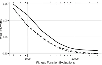
This paper aims at demonstrating the benefit of integrating into GP a surrogate model based on phenotypic characterization. The relative performance of a GP with and with-out surrogate model should be mostly independent of the GP parameter settings, as long as they are reasonable. The GP with surrogate model however uses an interme-diate population of larger size, so it seems sensible to investigate the influence of the population size.

0.90 0.95 1.00 1.05

1000 10000

Fitness Function Evaluations

Mean Flo

wtime

Figure 10: Convergence of Standard GP (solid curve), Surrogate-Assisted GP withn= 2 (dashed curve), and Surrogate-Assisted GP using a hypothetical perfect surrogate (dash-dot curve; also usingn= 2).

seems to be a good compromise for the maximum budget of 30,000 fitness evaluations used.

More important for the findings of this paper is the comparison between Standard GP and Surrogate-assisted GP for population sizes of 250 and 1,000 as shown in Fig-ure 9b. For both settings there is a clear benefit of using the surrogate, resulting in faster convergence as well as convergence to better performance levels. The benefits of using the surrogate model for a population size of 500 were already analyzed in more detail in the previous sections and shown graphically in Figure 7b. In summary, using the surrogate model appears to be beneficial independent of the population size used.

6.7 Perfect Surrogate

So far, we could demonstrate a clear benefit of Surrogate-Assisted GP in terms of con-vergence speed and concon-vergence level as compared to Standard GP. Now we would like to understand how much better we might be able to do by further improving the surrogate model. To answer this question we performed additional experiments for Surrogate-Assisted GP withn= 2. In these experiments, we replaced the calculation of the phenotypic characterization and surrogate evaluation with a full fitness evaluation. Of course this takes much more time, as we are performing 60,000 instead of just 30,000 fitness evaluations, but offers a lower bound, and allows us to assess the performance if we had a perfect surrogate model.

Results of these runs are shown in Figure 10. Solid and dashed curves show the performance of Standard GP and Surrogate-Assisted GP as already shown above. Re-sults for the hypothetical perfect surrogate are shown by the dash-dot curve. The two curves are very close which means that the surrogate model based on a rule’s phe-notyptic characterization, as used in this paper, is quite effective and, at least for the parameters investigated, allows to gain a large portion of the improvement potential over Standard GP.

7

Conclusion

a phenotypic characterization, we enable the use of surrogate models in combination with GP. The idea is to record the outcome of the rule encoded in a GP individual in a specified set of decision situations, and work in the space of phenotypic characteriza-tions rather than genotypes to construct and evaluate the surrogate model.

We have demonstrated the usefulness of our approach at the example of evolving dispatching rules for dynamic job shop scheduling. We present a phenotypic character-ization for this problem, and show how it can be used to detect (and remove) phentoyp-ically equivalent individuals, leading to a faster evolution of better solutions. We also show how the phenotypic characterizations can be used to successfully learn surrogate models that can be used to replace expensive fitness evaluations, further speeding up evolution. Together, our proposed approach saved up to 80% of the fitness evaluations compared to the standard GP model. The paper is thus an important advancement, al-lowing GP to be used for problems with computationally expensive fitness evaluations. A comparison with an alternative approach that uses a genotypic distance measure on the GP trees shows that the surrogate models built on phenotypic characterizations are much more accurate than those based on genotypic distances.

There are several ways to extend our work in the future. First, different modeling techniques can be investigated such as Neural Networks, Support Vector regression, or Gaussian Process regression. We expect such techniques to lead to even better surro-gate quality. Second, there are several ways to improve the model management and integration of the surrogate in the GP run. What training data to use and what indi-viduals to evaluate with the expensive fitness functions are currently handled in an effective, yet simple way, certainly allowing for further refinements and improvements in future work. Third, it would be interesting to further investigate the choice of de-cision situations that form the basis for the phenotypic characterization, and perhaps adapt these situations online during the run. Fourth, the idea should also be tested in other application domains, which would require to develop corresponding phenotypic characterizations. Last but not least it would be interesting to combine the work pre-sented in this paper with efforts to create improved GP operators incorporating seman-tic information, such as proposed by Uy et al. (2011), and fitness sharing incorporating semantic information (Nguyen et al., 2012). Both areas seem to be complementary to our work and can probably be combined to further improve the performance of GP in application areas with expensive fitness evaluations.

Acknowledgment

The authors would like to thank Alberto Moraglio for the source code to compute the Structural Hamming Distance (SHD) as a syntactic/genotypic similarity measure be-tween trees.

This work was partially supported by the German Research Foundation (DFG) under grant SCHO 540/17-2.

References

Ashlock, D., Lee, C., 2013. Agent-case embeddings for the analysis of evolved systems. IEEE Transactions on Evolutionary Computation 17 (2), 227–240.

dispatch-ing rules for manufacturdispatch-ing job shop operations. International Journal of Production Research 20 (1), 27–45.

Branke, J., Hildebrandt, T., Scholz-Reiter, B., 2013. Evolving dispatching rules—a com-parison of rule representations. Evolutionary Computation JournalSubmitted for publication.

Branke, J., Schmidt, C., 2003. Fast convergence by means of fitness estimation. Soft Computing Journal 9, 13–20.

Burke, E. K., Hyde, M., Kendall, G., Ochoa, G., ¨Ozcan, E., Woodward, J. R., 2010. A classification of hyper-heuristic approaches. In: Gendreau, M., Potvin, J.-Y. (Eds.), Handbook of Metaheuristics, 2nd Edition. Vol. 146 of International Series in Opera-tions Research and Management Science. Springer, New York, pp. 449–468.

Burke, E. K., Hyde, M. R., Kendall, G., Ochoa, G., ¨Ozcan, E., Woodward, J. R., 2009. Exploring hyper-heuristic methodologies with genetic programming. In: Kacprzyk, J., Jain, L. C., Mumford, C. L., Jain, L. C. (Eds.), Computational Intelligence. Vol. 1 of Intelligent Systems Reference Library. Springer Berlin Heidelberg, pp. 177–201.

Dimopoulos, C., Zalzala, A. M. S., 2001. Investigating the use of genetic programming for a classic one-machine scheduling problem. Advances in Engineering Software 32 (6), 489–498.

Ek´art, A., N´emeth, S. Z., 2000. A metric for genetic programs and fitness sharing. In: Proceedings of the European Conference on Genetic Programming. Springer-Verlag, London, UK, UK, pp. 259–270.

El-Beltagy, M. A., Keane, A. J., Nair, P. B., 1999. Metamodeling techniques for evolution-ary optimization of computationally expensive problems: Promises and limitations. In: Genetic and Evolutionary Computation Conference. Morgan Kaufmann, pp. 196– 203.

Emmerich, M., Giotis, A., ¨Ozdemir, M., B¨ack, T., Giannakoglou, K., 2002. Metamodel-assisted evolution strategies. In: Proceedings of the 7th International Conference on Parallel Problem Solving from Nature. PPSN VII. Springer-Verlag, London, UK, UK, pp. 361–370.

Geiger, C. D., Uzsoy, R., Aytug, H., 2006. Rapid modeling and discovery of priority dispatching rules: an autonomous learning approach. Journal of Scheduling 9 (1), 7–34.

Goel, T., Haftka, R. T., Shyy, W., Queipo, N. V., 2007. Ensemble of surrogates. Structural and Multidisciplinary Optimization 33 (3), 199–216.

Gustafson, S., Feb. 2004. An analysis of diversity in genetic programming. Ph.D. thesis, School of Computer Science and Information Technology, University of Nottingham, Nottingham, England.

Haupt, R., 1989. A survey of priority rule-based scheduling. OR Spektrum 11 (1), 3–16.

Hildebrandt, T., 2012. Jasima - an efficient Java Simulator for Manufacturing and Lo-gistics. Last accessed 16th September 2013.

Hildebrandt, T., Heger, J., Scholz-Reiter, B., 2010. Towards improved dispatching rules for complex shop floor scenarios: a genetic programming approach. In: GECCO ’10: Proceedings of the 12th annual conference on Genetic and evolutionary computation. ACM, New York, NY, USA, pp. 257–264.

Holthaus, O., Rajendran, C., 1997. Efficient dispatching rules for scheduling in a job shop. International Journal of Production Economics 48 (1), 87–105.

Holthaus, O., Rajendran, C., 2000. Efficient jobshop dispatching rules: further develop-ments. Production Planning & Control 11 (2), 171–178.

Hong, Y.-S., H.Lee, Tahk, M.-J., 2003. Acceleration of the convergence speed of evo-lutionary algorithms using multi-layer neural networks. Engineering Optimization 35 (1), 91–102.

Jackson, D., 2011. Promoting phenotypic diversity in genetic programming. In: Schae-fer, R., Cotta, C., Kolodziej, J., Rudolph, G. (Eds.), Parallel Problem Solving from Nature – PPSN XI. Vol. 6239 of Lecture Notes in Computer Science. Springer Berlin / Heidelberg, pp. 472–481.

Jin, Y., 2005. A comprehensive survey of fitness approximation in evolutionary compu-tation. Soft Computing - A Fusion of Foundations, Methodologies and Applications 9, 3–12.

Jin, Y., 2011. Surrogate-assisted evolutionary computation: Recent advances and future challenges. Swarm and Evolutionary Computation 1 (2), 61–70.

Jin, Y., Branke, J., 2005. Evolutionary optimization in uncertain environments-a survey. Evolutionary Computation, IEEE Transactions on 9 (3), 303–317.

Jin, Y., Huesken, M., Sendhoff, B., 2003. Quality measures for approximate models in evolutionary computation. In: Proceedings of GECCO Workshops: Workshop on Adaptation, Learning and Approximation in Evolutionary Computation. AAAI, pp. 170–173.

Jin, Y., Olhofer, M., Sendhoff, B., oct 2002. A framework for evolutionary optimization with approximate fitness functions. Evolutionary Computation, IEEE Transactions on 6 (5), 481–494.

Koza, J. R., 1992. Genetic Programming: On the Programming of Computers by Means of Natural Selection. MIT Press, Cambridge, MA, USA.

Law, A. M., 2007. Simulation Modeling and Analysis, 4th Edition. McGraw-Hill, New York, USA.

Lehman, J., Stanley, K. O., 2010. Efficiently evolving programs through the search for novelty. In: Genetic and Evolutionary Computation Conference. ACM, pp. 837–844.

Lim, D., Jin, Y., Ong, Y.-S., Sendhoff, B., june 2010. Generalizing surrogate-assisted evo-lutionary computation. Evoevo-lutionary Computation, IEEE Transactions on 14 (3), 329– 355.

Moraglio, A., Poli, R., sept. 2005. Geometric landscape of homologous crossover for syntactic trees. In: Evolutionary Computation, 2005. The 2005 IEEE Congress on. Vol. 1. pp. 427–434.

Nguyen, Q., Nguyen, X., O’Neill, M., Agapitos, A., 2012. An investigation of fitness sharing with semantic and syntactic distance metrics. In: Moraglio, A., Silva, S., Krawiec, K., Machado, P., Cotta, C. (Eds.), Genetic Programming. Vol. 7244 of Lecture Notes in Computer Science. Springer Berlin / Heidelberg, pp. 109–120.

Nguyen, S., Zhang, M., Johnston, M., Tan, K.-C., 2013a. Automatic design of scheduling policies for dynamic multi-objective job shop scheduling via cooperative coevolution genetic programming. IEEE Transactions on Evolutionary Computation.

URLDOI:10.1109/TEVC.2013.2248159

Nguyen, S., Zhang, M., Johnston, M., Tan, K.-C., 2013b. A computational study of rep-resentations in genetic programming to evolve dispatching rules for the job shop scheduling problem. IEEE Transactions on Evolutionary Computation 17 (5), 621– 639.

Oduguwa, V., Roy, R., 2002. Multiobjective optimization of rolling rod product design using meta-modeling approach. In: Genetic and Evolutionary Computation Confer-ence. Morgan Kaufmann, New York, pp. 1164–1171.

Pfund, M. E., Mason, S. J., Fowler, J. W., 2006. Semiconductor manufacturing schedul-ing and dispatchschedul-ing. In: Herrmann, J. W. (Ed.), Handbook of Production Schedul-ing. Vol. 89 of International Series in Operations Research & Management Science. Springer, New York, pp. 213–241.

Pickardt, C., Branke, J., Hildebrandt, T., Heger, J., Scholz-Reiter, B., 2010. Generating dispatching rules for semiconductor manufacturing to minimize weighted tardiness. In: Johansson, B., Jain, S., Montoya-Torres, J., Hugan, J., Y ¨ucesan, E. (Eds.), Proceed-ings of the 2010 Winter Simulation Conference. IEEE, New York, USA, pp. 2504–2515.

Pickardt, C., Hildebrandt, T., Branke, J., Heger, J., Scholz-Reiter, B., 2013. Evolution-ary generation of dispatching rule sets for complex dynamic scheduling problems. International Journal of Production Economics.

Poli, R., Langdon, W. B., Mcphee, N. F., March 2008. A field guide to genetic program-ming.

Rajendran, C., Holthaus, O., 1999. A comparative study of dispatching rules in dynamic flowshops and jobshops. European Journal of Operational Research 116 (1), 156–170.

Rattle, A., 1998. Accelerating the convergence of evolutionary algorithms by fitness landscape approximation. In: Parallel Problem Solving from Nature. Springer, pp. 87–96.

Runarsson, T. P., 2004. Constrained evolutionary optimization by approximate ranking and surrogate models. In: Parallel Problem Solving from Nature. No. 3242 in LNCS. Springer, pp. 401–410.