Orbital parameters estimation for compact binary stars

(1)

University of Warwick institutional repository: http://go.warwick.ac.uk/wrap

A Thesis Submitted for the Degree of PhD at the University of Warwick

http://go.warwick.ac.uk/wrap/75554

This thesis is made available online and is protected by original copyright.

Please scroll down to view the document itself.

(2)

Orbital Parameters Estimation for Compact

Binary Stars

by

Penélope Alejandra Longa-Peña, MSc

Thesis

Submitted to the University of Warwick for the degree of

Doctor of Philosophy

Department of Physics

(3)

List of Figures

1.1 Roche Potential . . . 3

1.2 Schematic representation of the accretion disc formation. . . 7

1.3 Schematic of CV evolution. Based on figure from Postnov & Yungelson (2014). Figure not to scale. . . 9

1.4 Orbital period distribution . . . 11

1.5 Mass transfer versus orbital period of CVs . . . 12

1.6 Superhump excess versus mass ratio. . . 14

1.7 Evolution of NS binaries . . . 16

1.8 Orbital phases . . . 18

1.9 Stars of massesM1andM2orbiting around their centre of mass. . . 18

1.10 Sodium spectra . . . 20

1.11 Blackbody radiation curves. Image created for educational purposes, courtesy of “Darth Kule”. . . 21

1.12 Disc’s double peaked profile formation . . . 22

1.13 Cataclysmic variable spectrum . . . 23

1.14 X-ray binary spectrum . . . 24

1.15 Trailed spectra of Sco X-1 from Steeghs & Casares (2002) . . . 25

2.1 Schematic of the essential components of a spectrograph . . . 29

2.2 MagE spectra of the X-ray binary Sco X-1. . . 30

2.3 Photograph of MagE installed on the Magellan II telescope. . . 31

2.4 MagE optical design. . . 31

2.5 MagE bias frame . . . 32

2.6 MagE flat field frame. . . 34

2.7 MagE ThAr lamp frame . . . 34

2.8 MagE spectra of V4140 Sgr . . . 36

2.9 Diagnostic diagram for CC Scl . . . 39

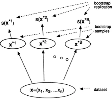
2.10 Schematic of the bootstrap process. . . 41

(7)

List of Figures v

2.12 Representation of the line profile formation process. . . 43

2.13 Schematic view of a CV in velocity coordinates. . . 44

2.14 Simulated data for 3 values ofγ . . . 46

2.15 Histograms of FWHM for two values ofγ. . . 49

2.16 FWHM and STD of the donor versus systemic velocity . . . 50

2.17 Residuals level againstK1. . . 51

2.18 Doppler map of CaII 8662 Å of CC Scl. . . 52

2.19 K1–qplane . . . 53

2.20 Location of different velocities on the donor surface . . . 53

2.21 Dependence ofKemand K-correction upon the inclination angle assumed in the model. 55 2.22 K1–qplane for two inclination angles . . . 56

2.23 Dependence ofKemand K-correction upon the disc height. . . 57

2.24 K1–qplane for two values ofK1 . . . 58

2.25 Synthetic data Doppler maps. . . 58

2.26 Gaussian spot of FWHM=40 km/s, S/N=2. . . 59

2.27 Gaussian spot of FWHM=40 km/s, S/N=25 . . . 60

2.28 Gaussian spot of FWHM=80 km/s, S/N=2 . . . 60

2.29 Gaussian spot of FWHM=40 km/s, accretion disc at the same intensity level, S/N=2. . 61

2.30 Gaussian spot of FWHM=40 km/s, accretion disc at the same intensity level, S/N=25 61 2.31 Gaussian spot of FWHM=40 km/s, accretion disc, intensity 5 times lower than the spot, S/N=25 . . . 61

2.32 Gaussian spot of FWHM=40 km/s, accretion disc, intensity 5 times lower than the spot, S/N=2 . . . 62

3.1 Average spectrum of CC Scl. . . 69

3.2 Average spectrum of V2051 Oph. . . 70

3.3 Diagnostic diagram of Hβfor V2051 Oph and CC Scl . . . 71

3.4 Radial velocity curves of Hα, Hβand CaII. CC Scl. . . 72

3.5 Radial velocity curves of Hα, Hβand CaII . . . 72

3.6 Two Doppler maps of Hβfor CC Scl generated with the same value ofχ2but with two different periods . . . 73

3.7 Doppler maps for CC Scl . . . 74

3.8 Doppler maps for V2051 Oph . . . 75

3.9 Histograms for two values ofγ . . . 76

3.10 FWHM of the secondary star and STD versus systemic velocity for CC Scl . . . 77

3.11 FWHM of the secondary star and STD versus systemic velocity for V2051 Oph. . . 77

(8)

vi List of Figures

3.13 K1velocity for five different boxes and six different lines . . . 80

3.14 Kemhistogram for CC Scl . . . 81

3.15 K1-q plane for CC Scl. . . 82

3.16 K1-q plane for V2051 Oph. . . 83

3.17 Doppler maps of the most prominent Balmer lines of V2051 Oph. . . 86

4.1 Two light curves of 4U1957 . . . 90

4.2 Comparison of the Bowen blend with different instruments . . . 93

4.3 Comparison of the Bowen blend with different instruments . . . 93

4.4 Average normalised spectrum of 4U 1957’s MagE data . . . 94

4.5 Diagnostic diagram of He II (top). Average spectrum of He II (bottom). . . 97

4.6 Periodogram for 4U 1957 . . . 98

4.7 Doppler maps of 4U 1957 . . . 100

4.8 Example Doppler maps of the Bowen blend, sub-set combinations . . . 101

4.9 Average, STD and average/STD from 500 bootstrap samples of the Doppler map of the Bowen blend . . . 101

4.10 FWHM and STD of the donor versus systemic velocity for 4U 1957 . . . 102

4.11 K1–qplane for 4U 1957 . . . 103

4.12 M1−M2plane for 4U 1957 . . . 105

5.1 Average Spectrum of AQ Eri UVB arm . . . 110

5.2 Average Spectrum of QZ Vir UVB arm . . . 110

5.3 Average spectrum of SDSS0137, UVB arm. . . 111

5.4 Average of 21 spectra of RZ Leo, UVB arm. . . 111

5.5 Average Spectrum of AQ Eri visual arm . . . 112

5.6 Average Spectrum of QZ Vir visual arm . . . 112

5.7 Average spectrum of SDSS0137, visual arm . . . 113

5.8 Average of 21 spectra of RZ Leo, visual arm. . . 113

5.9 Average Spectrum of AQ Eri NIR arm . . . 114

5.10 Average Spectrum of QZ Vir NIR arm . . . 114

5.11 Average spectrum of SDSS 0137, NIR arm . . . 115

5.12 Average spectrum of RZ Leo, NIR arm . . . 115

5.13 Diagnostic diagrams of AQ Eri . . . 118

5.14 Diagnostic diagrams of RZ Leo . . . 119

5.15 Doppler maps of AQ Eri . . . 121

5.16 Doppler maps of QZ Vir. . . 122

5.17 Doppler maps of SDSS0137 . . . 123

(9)

List of Figures vii

5.19 FWHM of the secondary star and STD versus systemic velocity for AQ Eri . . . 125

5.20 FWHM of the secondary star and STD versus systemic velocity for QZ Vir . . . 125

5.21 FWHM of the secondary star and STD versus systemic velocity for SDSS0137 using Hγ 126 5.22 FWHM of the secondary star and STD versus systemic velocity for SDSS0137 using CaII II 3933Å . . . 126

5.23 K1histograms . . . 127

5.24 K1-q plane for Aq Eri. . . 128

5.25 K1-qplane for QZ Vir . . . 129

5.26 K1-qplane for SDSS0137 . . . 130

6.1 ²−qplane with Knigge solution and our solution . . . 137

(10)

List of Tables

1.1 Types of compact remnants of single stars. . . 8 3.1 Orbital parameters derived from the diagnostic diagrams of CC Scl and V2051 Oph . 69 3.2 Orbital parameters summary . . . 87 4.1 Instruments performance comparison for the Bowen lines range. . . 91 4.2 4U 1957 MagE observations.nis the number of spectra taken during the given date. 92 4.3 4U 1957 IMACS observations.nis the number of spectra taken during the given date. 94 4.4 4U 1957 average equivalent width per night. MagE data . . . 95 4.5 4U 1957 average equivalent width per night. IMACS data. . . 95 4.6 4U 1957 orbital parameters derived from the diagnostic diagram of He II with MagE

and IMACS data. . . 96 5.1 X-shooter observation dates. . . 109 5.2 Orbital parameters derived from the diagnostic diagrams of AQ Eri, QZ Vir, SDSS0137

and RZ Leo.Φ0is relative to our ephemeris (Section 5.5). . . 116

5.3 Ephemeris andKem of the systems with a visible donor. . . 123 5.4 Primary velocity of the four systems calculated using the centre of symmetry technique.128

(11)

Acknowledgements

T here they stood, ranged along the hillsides, met To view the last of me, a living frame For one more picture! In a sheet of flame I saw them and I knew them all. And yet

Dauntless the slug-horn to my lips I set, And blew. ‘Childe Roland to the Dark Tower came.’

-Robert Browning, Childe Roland to the Dark Tower came.

And on an epic quest of my own I blow the slug-horn at the end of an epic journey. For all the things I’ve lost on my way here, some I’ll miss but I’ll never regret: To my friends lost in one way or another and the sacrifices of many people that helped me to be writing here today, I acknowledge. But I found many things in this journey, the most important one, my family: my husband and son that stood along through wind and rain and made it sunshine and spring. New friends that supplied me with support, coffee, spelling checks, CRISPS and non scientific palaver (yes, my PhD student’s party) and that made my life much easier with their youth of soul. And for these I’m grateful.

For the most important part of this journey, my journey to knowledge, I owe special gratitude to my supervi-sor Danny Steeghs for his valuable scientific advice, and for always been willing to share his ideas, a cup of coffee and a good laugh. I also would like to thanks to all the academics from the Astronomy group at the University of Warwick for the stimulating environment and additional supervision. A special mention to my former supervisor and friend Eduardo who always stood strong and showed me that I could fight harder than I believed that I was capable of my self.

I would like to thank Chris Copperwheat for the reducing the data used in Chapter 5.

Also, a HUGE thank you to my thesis correctors Boris and Chris for their very useful and thorough comments. I still like you =)

I stand today facing my destiny at the end of my quest. What awaits for me now that I’ve arrived, is to be revealed. The trip is always more important than the destiny. And what a trip it was!

‘T hink first, fight afterwards’... Stand and be true, I will be a Knight1.

1_{Well, a Doctor. But that is epic enough ;)}

(12)

(13)

Declaration and Published Work

I, Penelope Alejandra Longa-Peña, herby declare that the work presented in this thesis is my own except where references stated otherwise. This thesis has not been submitted either wholly or in part in any previous application for a higher degree in this or any other academic institution. The following Chapters are based on published refereed publications:

Chapter two, Section 2.4.7, & Chapter three:

“Emission line tomography of the short period cataclysmic variables CC Scl and V2051 Oph”

P. Longa-Pena; D. Steeghs; T. Marsh

Monthly Notices of the Royal Astronomical Society 2014 447 (3): 149-159

Chapter four:

“Dynamical Constraints for the Low Mass Black Hole Candidate 4U 1957+111”

P. Longa-Pena; D. Steeghs; R. Cornelisse; J.M. Miller; J. Casares, P.A. Charles In Preparation.

Some of the MagE data reduced as described in Chapter 2 has been published in:

“The unseen population of F- to K-type companions to hot subdwarf star”

Girven, J.; Steeghs, D.; Heber, U.; Gänsicke, B. T.; Marsh, T. R.; Breedt, E.; Copperwheat, C. M.; Pyrzas, S.; Longa-Peña, P. Monthly Notices of the Royal Astronomical Society 2012 425 (2): 1013-1041

“A Dynamical Study of the Black Hole X-ray Binary Nova Muscae 1991”

Jianfeng, W.; Orosz, J.A. ; McClintock, J. E.; Steeghs, D.; Longa-Peña, P.; Callanan, P.J. ;Gou, L.; Ho, L. C.; Jonker, P.; Reynolds, M.; Torres, M.

Accepted in The Astrophysical Journal.

(14)

(15)

Abbreviations

BH: Black hole

Ca: Calcium

CB: Compact binary CN: Classical Nova

CCD: Charge-Coupled Device C/O: Carbon/Oxygen

CRTS: Catalina Realtime Transient Survey CV: Cataclysmic Variable

ESO: European Southern Observatory FWHM: Full-Width at Half Maximum

H: Hydrogen

He: Helium

HST: Hubble Space Telescope INT : Isaac Newton Telescope LMXB: Low mass x-ray binary MagE: Magellan Echellette NIR: near-infrared

SDSS: Sloan Digital Sky Survey S/N: Signal to noise ratio STD: Standard Deviation VIS: visible

VLT: Very Large Telescope WD: White Dwarf

WHT: William Herschel Telescope

(16)

(17)

Abstract

Most stars in the Galaxy are found in multiple systems of two or more stars orbiting together. Two stars orbiting around their centre of mass are called binary stars. In close binary stars, the evo-lution of one star affects its companion and evoevo-lutionary expansion of one star allows for mass exchange between the components. In most cases, the material from the less massive star forms an accretion disc around the heavier companion that has evolved into a compact stellar rem-nant, the final state of stellar evolution. We call these systems compact binary stars (CBs). The study of CBs is key to the development of two fundamental phenomena: accretion and evolution of binary stars.

Statistical information on CBs can be deduced by extracting common properties and characteristic system parameter distributions from observed data. But, despite being funda-mental for a wide range of astronomical phenomena, our comprehension of their formation and evolution is still poor, mainly because of the limited knowledge of crucial orbital parameters. This lack of reliable orbital parameters estimation is mainly due to observational handicaps, namely, the accretion disc outshines the system components. Astronomers have developed dif-ferent techniques to overcome this, but are often very dependant of the signal to noise ratio of the data or are only able to obtain via target of opportunity programs (wait until the target is brighter).

The focus of this work is to test and develop techniques, based on indirect imaging meth-ods, that can overcome the main observational handicaps to estimate orbital parameters of CBs. We combine these techniques with the exploitation of more “exotic” emission lines that trace the irradiated face of the donor star, namely Ca II NIR triplet and the Bowen blend. We made use of empirical properties of Doppler tomography to estimate the values of the phase zeroφ0and

the velocity of the irradiated face of the secondary star (Kem). We then used synthetic models accounting for an irradiated secondary to fit our measuredKem and perform a K-correction to derive the radial velocity of the secondaryK2. To deriveK1, we used the centre of symmetry

tech-nique, testing its validity among several emission lines and the stability of the results depending on the selected area. Having strong constraints forK1andK2, we find estimates for the mass

ra-tioq. Furthermore, we developed a variation from the Doppler tomography secondary emission method to constrain the value of the systemic velocityγ. We derive meaningful uncertainties of

(18)

xvi List of Tables

these parameters with the bootstrap technique.

(19)

One

Introduction

Only around half of the stars that we see when we look to the sky are single stars. The rest are multiple systems, consisting of two or more stars orbiting around each other due to their grav-itational attraction. Two stars orbiting each other are called binary stars. Measurements of the dynamical interaction of the components in eclipsing binary stars provide the most accurately determined parameters of stars.

This work will focus on a particular class of binary: compact binary stars (CBs), consisting of a main sequence star and a stellar remnant- white dwarf (WD), neutron star (NS) or black hole (BH). These are considered primary targets for the forthcoming field of gravitational wave astronomy, since their orbital evolution is partially controlled by the emission of gravitational waves and ultimate leads to merging and possible explosive disruption of the components (for a review, see Thorne et al. 1987).

In Section 1.1 I will review the basics of binary geometry, evolution, classification and parameters. In Section 1.2 I will present some basics of spectral line formation and common features of CBs. Finally, in Section 1.3 I will present the advantages of the Bowen blend and the Ca II triplet to trace the secondary star in CB systems.

1.1 Compact Binary Stars

As the time scale of evolution of a star is largely dependant on its mass, the more massive the star the faster it evolves from the main sequence hydrogen burning phase to a stellar remnant. The initial (main sequence) mass of a star will determine how it will end its life:∼1M_¯stars will end their lives as a WD, stars of more than∼8M¯will end up as either NSs or BHs. In close binary stars, the evolution of one star affects its companion. Evolutionary expansion of stars allows for mass exchange between the components. In most cases, the material from the less massive star feeds an accretion disc around the heavier companion that has evolved faster to a compact stellar remnant, the collapsed end state of stellar evolution. We call these systems compact binary stars (CBs).

The study of the structure of CBs is key to the development of three fundamental phe-nomena: accretion flow, discs and the evolution of binary stars. The theory of accretion is

(20)

2 CHAPTER 1. INTRODUCTION

portant for the study of quasars, active galactic nuclei and even for planet formation. Due to the shorter timescales and distances with respect to these sources, observational research of the accretion process can be studied more effectively in compact systems such as CBs (see Frank & Raine 2002).

CBs are also the key to a wide variety of astrophysical phenomena from short gamma -ray bursts (Paczynski 1986, Berger et al. 2005, Gehrels et al. 2005), pulses of gravitational-waves emitted by stellar black holes (Casares et al. 1992), to the basis of the 2011 Nobel Price in physics (Riess et al. 1998, Schmidt et al. 1998, Perlmutter et al. 1999): Type Ia supernovae, whose progen-itors are WD binaries (Whelan & Iben 1973, Woosley et al. 1986, Ruiz-Lapuente et al. 2004).

Statistical information on CBs can be deduced by extracting common properties and characteristic system parameter distributions from observed data. Unfortunately, our under-standing of their formation and evolution is still poor, mainly because of the limited quantity of statistically significant CBs parameter samples. In recent years, surveys such as the Sloan Digital Sky Survey and Chandra have helped to fill this gap. Nevertheless, as we will show in the fol-lowing sections, to test population models and understand properties of many CVs, we still lack crucial orbital parameters for a large enough sample.

1.1.1 Binary Geometry

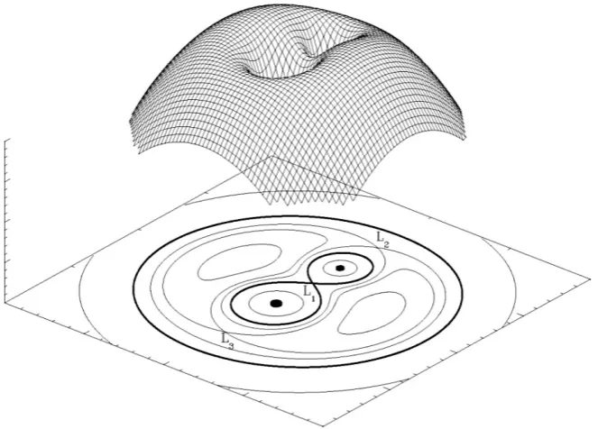
Given the potential function,Φ(r), we can draw a surface on which the potential is constant (Φ(r)=C, withC=constant). Such a surface is called an equipotential surface (see Figure 1.1).

Any flow of gas between two stars will be governed by the Euler equation (Frank & Raine, 2002):

ρ∂v

∂t +ρv· ∇v= −∇P+f (1.1)

whereρis the density,vis the velocity,Pis pressure andfis the external force. In our case,f are the centrifugal and Coriolis forces if we consider a frame of reference that rotates with the binary with an angular velocityωwith respect to an inertial frame:

∂v

∂t +(v· ∇)v= −∇ΦR−2ω×v−

1

ρ∇P (1.2)

where−2ω×vis the Coriolis force per unit mass and−∇ΦRincludes the effect of the centrifugal and gravitational forces.

For a binary system with massesM1andM2,ΦR is known as the Roche potential and is given by:

ΦR(r)=−

G M1

|r−r1|−

−G M2

|r−r2|−

1 2(ω×r)

(21)

[image:21.595.166.498.121.359.2]

1.1. COMPACT BINARY STARS 3

Figure 1.1: 3-D representation of the Roche potential forq=2. The equipotential surfaces are outlined in black in the lower plane. Figure from Postnov & Yungelson (2014).

where G is the universal gravitational constant andr1=

p

x2₊_y2₊_z2_and_r

2=

p

(x−1)2₊_y2₊_z2

are the position vectors of each star with respect to the centre of mass(Frank & Raine, 2002). The mass ratioqdetermines the shapes of the Roche equipotential and is given by:

q=M2

M1 =

K1

K2

(1.4) whereM1,M2,K1andK2are the masses and radial velocity semiamplitudes of the primary

(com-pact) and secondary (donor) star, respectively. The binary separationais given by Kepler’s law as:

P_{or b}2 = 4π

2_a3

G[M1+M2]

(1.5) wherePor bis the orbital period of the system.

From equations 1.3 and 1.5, the normalised Roche potential is then:

φn= − 2φ

G(M1+M2)=

2

r1(1+q)+

2q

r2(1+q)+

µ

x− q

1+q ¶2

+y2, (1.6)

showing explicitly the direct relation of the Roche potential and the mass ratio.

(22)

point markedL1, the inner Lagrangian point, the force exerted on a test particle co-rotating with

the binary vanishes, so the particle can escape from the surface of one star and be captured by the companion. In a CB, the matter escapes throughL1, and in the case of non magnetic CBs, as

the matter comes with a given angular momentum it forms a disc orbiting the companion. We call this process Roche-lobe overflow (RLOF) and it begins when the radius of an initially more massive (and hence faster evolving) star, becomes equal to the radius of the Roche lobe.

1.1.2 Evolution: Common Envelope and Stable Mass Transfer

Despite being a key stage for the formation of a CB, the common envelope stage remains poorly understood. One theory proposes that when the mass transfer rate from the donor star is too high for the companion to accommodate all the accreting material, the overflowing material be-comes an envelope that engulfs the whole system (e.g. Benson (1970), Neo et al. (1977), Webbink (1977) and Prialnik & Livio (1985)). Another possibility is the formation of an extended envelope formed over the system due to unstable nuclear burning of an accreting WD in the compact bi-nary (e.g. Starrfield et al. (1974), Paczynski & Zytkow (1978) and Nomoto et al. (1979)). A third scenario is when the donor star cannot keep synchronous rotation with the compact compan-ion, forcing the compact object to spiral into the envelope of a giant donor (Sparks & Stecher, 1974). Despite of all these uncertainties, the dramatic decrease of angular momentum experi-enced in the course of a CB’s evolution is compelling evidence of the existence of the common envelope stage.

Stable mass transfer depends on the balance between the response of the donor to mass loss, changes of separation and loss of angular momentum. Three time scales are important to regulate this process: the dynamical, thermal and nuclear time scales of the secondary. The dynamical time scale, on which the star reacts to departures from hydrostatic equilibrium is :

tdyn=

s

2R3

G M. (1.7)

For the Sun this is∼1600s, meaning that if the internal pressure of the Sun were removed, it would take this time to collapse. This time is roughly the time that a sound wave requires to cross the Sun.

The thermal timescale, on which the star reacts to departures from thermal equilibrium is de-fined as:

tth=

G M

RL , (1.8)

whereLis the luminosity of the star. For the Sun, this is∼3x107yr. This is the timescale on which the Sun would contract if its nuclear energy sources were turned off.

(23)

tnuc=(7x109)

M

M_¯

L¯

L year s. (1.9)

For the Sun this is∼109yr, the time required to exhaust all the Sun’s hydrogen at its cur-rent luminosity.

Neglecting the orbit’s eccentricity the angular momentumJ is given by (Landau & Lif-shitz, 1969):

J=M1M2

M a

2_Ω

orb (1.10)

whereMis the total mass of the system,M1is the primary star,M2is the mass donnor,ais the

orbital separation andΩorb(r)=£G M_r3 ¤1/2

is the Keplerian orbital velocity. The rate of change in the orbital separationais:

˙

a

a =2

˙

J

J−2

˙

M1

M1−

2M˙2

M2 =

2 ˙J

J −

2 ˙M2

M2

µ

1−M2

M1

¶

. (1.11)

If we conserve the angular momentum, ˙J =0, whenM2<M1: a_a˙ >0 and the orbit

ex-pands.

As the most massive star evolves first, mass transfer will always begin withM2>M1(note

that the definition ofM1andM2will reverse temporarily). AsM1is unable to adjust its structure

rapidly enough to maintain itself in the Roche lobe, mass transfer proceeds on the dynamical time scale, saturating and growing to form a common envelope around the stellar components. Inside the common envelope, the stars will spiral toward each other until enough orbital energy has been released to expel the envelope, delivering a barely detached system. Now, while the secondary evolves and eventually fills its Roche lobe,M2<M1and stable mass transfer on the

nuclear time scale, will occur. As the mass ratio changes, the Roche geometry adjusts accordingly to the new system parameters. The response of the secondary to these changes will determine the nature of the mass transfer. If the secondary outer layers are radiative, the donor has to ex-pand to maintain the mass transfer, having enough time to restore thermal equilibrium. On the other hand, if the secondary’s outer layers are convective, the Roche lobe can expand sufficiently to remain comparable in size to the stellar radius and the mass transfer will occur on the nuclear timescale (de Loore, 1992).

1.1.3 Accretion Disc

(24)

thatRcirchas the same angular momentum asL1.Rcircis called the circularization radius and

is defined as (Frank & Raine, 2002):

Rcirc

a =(1+q)[0.0500−0.227 logq]

4 _(1.12)

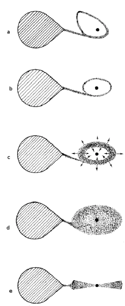
Figure 1.2 summarises the disc formation process by RLOF (see Verbunt 1982 and refer-ences therein). The matter does not hit the star directly, but flows around it until it hits the stream again (Figure 1.2a). The shock changes the flow of the stream into a circular shape (Figure 1.2b). The stream spreads into a disc due to viscosity, transporting matter inwards and outwards to pre-serve angular momentum (Figure 1.2c). The expansion of the disc continues until the outward disc is stopped by tidal interactions with the donor and the inner edge of the disc reaches the surface or magnetosphere of the compact object and starts to accrete (Figure 1.2d). Figure 1.2e is a side view of the accretion disc.

1.1.4 Angular Momentum Loss

The angular momentum term of Equation 1.11 accounts for the total loss in angular momentum from magnetic braking and gravitational radiation. Here, we will show the classic mathematical treatment of these two mechanisms. However, Knigge et al. (2011) have suggested that a better description of the evolution of CVs was reached by scaling the classical equations (that we will show below), by numerical factors, see the paper for details.

Magnetic Braking

The rotation of the secondary star is tidally locked to the orbital period, forcing it to rotate faster than a similar type single star. This fast rotation leads to highly magnetic secondaries. Charged particles flow through the field lines and are forced to co-rotate with the secondary, accelerating them. When these particles are released, they take with them substantial angular momentum in proportion to the orbital velocity of the systemΩorb(Verbunt & Zwaan, 1981)

˙

JM B

J ∝ −f

−2

M B

k2R₂4

a2

M

M1Ω

2

orb (1.13)

wherekis the radius of gyration of the part of the star coupled to the magnetic wind andk2=0.01 (Verbunt & Zwaan, 1981). fM B is an empirically determined factor varying betweenfM B =0.73 (Skumanich, 1972) andfM B=1.78 (Smith, 1979).

(25)

[image:25.595.226.440.154.677.2]

con-1.1. COMPACT BINARY STARS 7

(26)

Initial mass [M_¯] remnant type typical remnant mass [M_¯]

0.95<M<8−12 WD 0.6

8−11<M<25−30 NS 1.35

20<M<150 BH ∼10

Table 1.1: Types of compact remnants of single stars. Table reproduced from Postnov & Yungel-son 2014.

tact with its Roche lobe and the main angular momentum loss mechanism will be gravitational radiation.

Gravitational Radiation

General relativity predicts that matter curves space and that the acceleration of a binary system causes ripples in the fabric of space, moving outwards in a periodic wave, a gravitational wave. The energy and angular momentum carried by these ripples is extracted from the binary orbit, causing the system to spiral inwards. The rate of angular momentum loss due to gravitational radiation is given by (Landau & Lifshitz, 1969):

˙

JGR

J = −

32 5

G4

c5

M₁2M₂2M

a4 (1.14)

For wide compact binaries with WD primaries, relativistic effects are weak, but as the stars orbit closer and faster, gravitational radiation dominates, becoming the main angular mo-mentum loss mechanism (Warner, 1995).

1.1.5 Compact Binaries Classification

Compact binaries (CBs) are the end product of the evolution of stellar binaries. They typically consist of a lower mass main-sequence star and a compact object, but there are also double degenerate binaries, with two compact objects. The resulting CB depends on the initial mass of the compact object progenitor,M0. If M0is lower than the minimum mass required to ignite

carbon in the core, then after the hydrogen and helium have burnt the star becomes a WD. IfM0

exceeds a certain mass, the star produces an iron core, which collapses into a NS or a BH. The boundaries between the masses of the progenitors are fairly uncertain, being usually accepted, for solar composition single stars, as the ones shown in Table 1.1.

Cataclysmic Variables

(27)

[image:27.595.119.556.73.570.2]

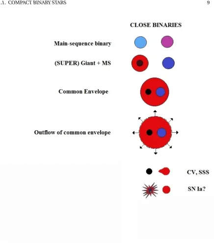
Figure 1.3: Schematic of CV evolution. Based on figure from Postnov & Yungelson (2014). Figure not to scale.

the name “cataclysmic” to their outbursts, observed as modulations in the light curve of the sys-tems. Their prevalence makes CV populations particularly useful for improving our understand-ing of accretion and compact binary evolution. Figure 1.3 shows a schematic of the evolution of CVs.

(28)

• Dwarf Novae: These systems present outbursts that temporarily increases their brightness by 2-5 magnitudes (see Section 1.1.5). These outbursts last∼2−20 days , recurring on periods ranging from days to several decades. Outbursts are understood as instabilities that take place in the accretion disc, enhancing the accretion on to the surface of the pri-mary star which as a consequence increases the system’s brightness. The accretion disc, which in outburst is hot and large, shrinks between outbursts, reaching a cool state called quiescence. The dwarf novae group is further subdivided into three categories:

– SU UMa: These systems exhibit super outbursts, which are about 5 times longer and brighter than regular outbursts (see Section 1.1.5).

– Z Cam: These systems exhibit a mixture of outbursts and standstills, remaining for long periods at∼0.7 magnitudes below their maximum brightness.

– U Gem: All the other dwarf novae that are neither SU UMa nor Z Cam.

• Classical novae: These systems have only been observed to have one eruption. We call this a nova eruption as they are thermonuclear runaways oiginated in the WD surface.

• Recurrent novae: These are systems which originally were classified as classical novae but then a new eruption was observed. Ejection of a shell from the primary stars’s surface is observed in spectroscopic data from recurrent novae, separating them from the dwarf novae category.

• Nova-likes: These are all of the non-eruptive CVs with high accretion rates ( ˙M)

Magnetic CVs are classified into two groups, based on the effect the magnetic field of the WD has on the formation of the accretion disc:

• Polars: The WD’s magnetic field is so strong that no disc is formed, so the material donated by the secondary accretes onto the poles of the white dwarf, following the magnetic field lines.

• Intermediate polars: These systems have discs that are truncated at the inner edge, where the WD’s magnetic field is strong enough to completely disrupt the accretion disc.

Our research will focus on SU UMa type CVs that typically dominate at short orbital pe-riods (shorter than 2 h).

(29)

[image:29.595.231.441.120.327.2]

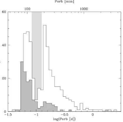
Figure 1.4: Orbital period distribution of 454 CVs from Ritter & Kolb (2003) which have no spec-troscopic observation in SDSS DR6 (white) and the distribution of 137 SDSS CVs from Gänsicke et al. (2009) (gray). The gray shaded area represents the 2–3 h orbital period gap. Figure from Gänsicke et al. (2009).

the orbital period distribution from Gänsicke et al. (2009). There are 3 pronounced features that can be explained by the CV evolution models. These are: a sharp cut-off at short orbital periods, known as the period minimum, a deficit of systems in the 2-3 hours regime (grey shaded area), known as the period gap, and a diminishing number of CVs at long orbital periods.

First, notice that for orbital periods above∼12 hours (-0.3 log(d) in the figure) the num-ber of systems considerably decreases. This is a result of the requirement that the secondary be less massive than the WD for stable mass transfer. The systems are then limited by the Chan-drasekhar limit of a WD being≤1.4M_¯; the mass of the secondary is also constrained by this limit. As the size of the binary increases with orbital period, so does the size of the secondary’s Roche lobe. Larger Roche lobes require larger secondaries to fill them, setting the∼12 hours limit on the orbital period.

(30)

[image:30.595.232.426.116.264.2]

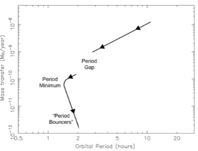
Figure 1.5: Mass transfer versus orbital period of CVs. Evolution proceeds from magnetic braking (MB) above the gap, and then by gravitational radiation (GR) below the gap (from Hellier (2001))

Angular momentum loss by magnetic braking (Rappaport et al. 1983) and gravitational radiation (Paczynski & Sienkiewicz 1981) drives CVs to shorter periods while the donor is trans-ferring mass (see Figure 1.5). When the mass of the donor becomes too low to sustain hydrogen burning, it becomes degenerate, causing the orbital period to increase and hence we have a min-imum orbital period (see Section 1.1.2 and 1.1.4).

It is believed that a large percentage of CVs should have evolved towards short orbital periods (∼80 min). At this so-called period minimum, when the donor becomes degenerate, it no longer shrinks, but it expands in response to mass loss, and the period evolution reverses sign, leading to a period increase. Thus a CV is expected to spend a significant fraction of its time with an orbital period near the period minimum. Because of this, a significant accumulation of CVs at the minimum period is expected. This accumulation is often called the ‘period minimum spike’ (e.g. Kolb & Baraffe 1999). Two families of CVs are expected to coexist near the period minimum, one evolving from longer periods down towards the period minimum and the other one that has reached the minimum and is evolving out to longer periods (see Figure 1.5). The key difference between both families lies in the mass of the donor star. The first family is expected to have low mass main sequence stars, while on the second one, the donor has evolved towards much lower masses and resembles a brown dwarf.

(31)

of individual systems is needed, particularly, the masses of the components. The measurement of the superhump period (read further along this Section for the definition) could potentially provide an indication of the mass ratio of the systems via the empirical relation between the two observables (Pearson, 2006), but is poorly constrained at the short orbital periods end (see above).

While the standard CV evolution model can explain the bulk features of the CV period distribution, more quantitative comparisons between evolutionary models and the CV popula-tion are desired, in particular for those systems where more than just the binary period is known. Theoretical models of the evolution of CVs predict the distribution of their orbital parameters: orbital periods, mass ratioq=M2/M1and the individual masses of the two stars,M1+M2.

Re-grettably, too often the only reliable physical parameter that can be measured for most CVs is their orbital period, since the faint donor stars and cool WDs are difficult to find. In order to val-idate the theory and pinpoint the evolutionary track of CVs – evolving towards (pre-bounce) or from the period minimum (post-bounce)– more information about the parameters of individual systems is needed. Particularly, the mass of the secondary star can differentiate a pre- from a post-bouncer as the evolution of CVs is controlled by the properties of their secondaries (Knigge et al., 2011).

Dwarf Nova Outbursts The standard theory to explain the disc outbursts is a thermal-viscous instability that occurs in the accretion disc, called the disc instability model (Osaki, 1974). The viscosity is given by the so calledα-prescription, where the viscosity is given by (Shakura & Sun-yaev, 1973):

v=αcsH (1.15)

whereαis a number less than one,His the vertical height of the disc andcs is the sound speed in the gas. The instability arises when hydrogen becomes partially ionised and the disc opacity varies with temperature. A number of characteristics of many light curves are reproduced by the disc instability model if we assume that the viscosity parameterαis different in quiescence and in outburst.

(32)

0.05 0.10 0.15 0.20 0.25 0.30

mass ratio

q

=

M

₂

/M

₁ 0.00 0.01 0.02 0.03 0.04 0.05 0.06 0.07 0.08

su

pe

rh

um

p

ex

ce

ss

²

= (

P

S −

P

O )

/P

O WZ Sge XZ Eri OY Car

Figure 1.6: A CV superhump period is slightly in excess with respect to its orbital period. The figure shows that the fractional period excess appears to be correlated with the mass ratio “q” for the small number of systems with independent mass ratio estimates. This has potentially led to the use of the superhump period excess as an estimator of the mass ratio of many CVs. However, the low mass ratio end (q <0.12) is poorly calibrated. The dashed line indicates the currently employed empirical conversion from superhump excess to “q”.

of the secondary slows the bulge, reducing its angular momentum thus helping the material to flow inwards in the disc. In equilibrium, this bulge would orbit slightly ahead of the secondary. However, if the secondary’s tidal interaction resonates with the radial motion of the disc, it will enhance the radial component of the motion, driving the outer disc elliptical. The most common resonance excited is 3:1, but in more extreme mass ratio systems, 2:1 can also be excited. As the elliptical orbits are no longer parallel to the circular inner orbits, these now intersect and cause collisions that result in energy dissipation and an enhanced emission in the system’s light curve. This emission appears as a hump-shaped modulation when the system reaches the peak of the super-outburst. Superhumps are commonly seen in CVs, and are discussed in more detail by Warner (1995), and can also occur in low mass X-ray binaries (LMXBs, Section 1.1.5).

(33)

ratio vary by more than a factor of two and thus its use as a calibrator may be questioned. The dashed line indicates the currently employed empirical conversion from Knigge (2006). One of the aims of this work is to identify new calibrators for this empirical relation, especially in the low mass ratio end, and test the validity of the relationship.

X-ray Binaries

X-ray binaries come in a diverse range of systems, the most common division made between binaries with low or high mass secondary stars: low mass X-ray binaries (LMXB) and high mass X-ray binaries. This work will only concern LMXBs as these share the geometry of CVs but with a NS or BH as the compact object. Observationally, we can differentiate LMXB, into persistent and transient sources. In quiescent transient sources, the light usually becomes dominated by the secondary, allowing radial velocity studies to measure the system parameters, particularly the compact object mass. This is not possible in persistent sources.

Yet another important distinction is made between systems containing NSs or BHs. This classification is important, since many similarities can be found in the behaviour of low mass and high mass X-ray binaries. Both NS and BH binaries are descendants of initially massive bi-naries (Postnov & Yungelson, 2014). Figure 1.7 presents the standard evolutionary scenario for the formation of NS or BH binaries, from main sequence to potential merging of the compo-nents; see text in the Figure for details.

As we mention in Section 1.1.5, LMXBs can also exhibit superhumps. The most likely LMXBs to exhibit superhumps are BH systems since they have more extreme mass ratios than most NS LMXBs. The superhump mechanism in LMXBs is different than the one operating in CVs. As the optical light in a LMXB is not dominated by viscous dissipation, but by irradiation by X-rays, the superhumps arise from coupling of irradiation to tidal distortion of the disc (e.g. Haswell et al. 2001).

1.1.6 Orbital Parameters

In this section, we will present some of the physical parameters of CBs.

Orbital Period

(34)

(35)

a given range of periods simultaneously, allowing for random contributions to disappear (except for the ones generated by the data collection itself ). The test function is defined as:

Px(ω)=

1 2

h P

jXjcos(ω)(tj−τ) i2

P

jcos2(ω)(tj−τ) + h

P

jXjsi n(ω)(tj−τ) i2

P

jsi n2(ω)(tj−τ)

(1.16) wheretjare the sample times,Xj are the time series data,τis the time delay and is given by:

tan(2ωτ)= P

jsin(2ωtj) P

jcos(2ωtj)

andωis the candidate frequency, the inverse of the candidate period.

In practise, aliases and some orbital dependant variations (e.g. pulsations, elliptical discs), complicate the task of finding an accurate orbital period. Despite this, often enough, the orbital period is the only well determined orbital parameter for many CBs.

The plot of the candidate periods versus the test function is called a “periodogram”, hence the name of the technique.

Phase Zero

When the binary star orbits around its centre of mass, depending on its relative position with respect to the observer, it goes through different phases. When the primary star is aligned with the centre of mass and the secondary is between it and the observer, we call it phase zero or conjunction, as shown in Figure 1.8. Orbital phases go from 0 to 1. In Figure 1.8, we marked phases 0.25, 0.5, and 0.75, increasing anticlockwise. When the primary reaches phase zero again, this will now be phase 1 from the current orbital cycle and phase zero of the next cycle.

Inclination and Masses

Figure 1.9 shows the orbit of two massesM1andM2with an orbital periodPor b and a centre of mass separation ofa=a1+a2, wherea1M1=a2M2. The inclination angle is usually measured

between the orbital plane of the system and the plane of the observer (ecliptic), perpendicular to the line of sight. If we observe the system with an inclinationi, then the orbital velocity projected along the line of sight will be:

K1=

2πa1

Por b

siniand K2=

2πa2

Por b

sini (1.17)

for the primary and secondary, respectively. We will discuss how to measure these velocities in Chapter 2.

Combining 1.17 with Kepler’s third law, Eq. 1.5, we obtain: (M2sini)3

(M1+M2)2=

Por bK₁3

(36)

Figure 1.8: Orbital phases. The centre of mass is marked as C.M.

Figure 1.9: Two stars of massesM1andM2orbiting in a plane around their common centre of

mass. The arrow points towards the observer, defining the inclination anglei.

and

(M1sini)3

(M1+M2)2=

Por bK₂3

2πG (1.19)

wherea=a1

³_M 1+M2 M2

´

. Dividing these two equations, we obtain the mass ratio as in Eq. 1.4. If the orbital period is known, we still would need the system inclinationito determine the mass ratio. The standard method to estimate the masses of a binary with a known orbital period is to measureK1,K2andi or to measure two of these three and another restriction (e.g.

q).

1.2 Spectral Line Formation

(37)

1.2. SPECTRAL LINE FORMATION 19

element alone, allowing us to study the composition of celestial objects with spectral analysis. Figure 1.10 shows the spectra of Sodium in emission and absorption. To understand the differ-ences between these two spectra, we must remember some basic quantum mechanics: given the Plank-Einstein relation:

E=hc

λ (1.20)

where h is the Planck’s constanth=6.62606876e34 J s (Carrol & Ostlie, 2007). This relation shows that the energy of a photonE is inversely proportional to its wavelengthλ. The wavelength is related to the frequency (ν) asλ=c/ν. Given Bohr’s frequency condition:

∆E=hν (1.21)

where∆Eis the energy difference between two energy levels involved in an electronic transition. When the electron jumps from one level to another, the atom emits or absorbs a pho-ton of energy equal to the difference in energy between the two levels. From Equation 1.20, if two photons have the same energy, they must also have the same wavelengthλ. Hence, if an atom can emit photons of a certain wavelength, it can also absorb photons of precisely the same wavelength, explaining what we see in Figure 1.10; a hot, dense gas or solid object produces a featureless continuous spectrum, a blackbody. A hot, diffuse gas produces bright emission lines. These are produced when an electron jumps from a higher to a lower orbit. The energy lost is carried away by a single photon that has two ways to decay: to ground state or to cascade one orbital at a time. A cool, diffuse gas in front of a source of continuous spectrum produces dark absorption lines in the continuous spectrum. These are produced when an electron jumps from a lower to a higher energy level, absorbing a photon that carries exactly the amount of energy equal to the difference in energy between the higher orbit and the electron’s initial orbit.

These observations are summarised in Kirchhoff’s laws (Kirchhoff, 1860):

1. A hot opaque body, such as a perfect blackbody, or a hot dense gas produces a continuous spectrum.

2. A hot transparent gas produces an emission line spectrum.

3. A cool, transparent gas in front of a source of a continuous spectrum produces an absorp-tion line spectrum.

(38)

Figure 1.10: Emission and absorption spectra of Sodium.

permitting us to deduce how fast stars and other objects are approaching or receding. Measur-ing the non-relativistic Doppler shift of spectral lines can be used to determine the star’s radial velocity (vr):

λobs−λrest

λrest =

∆λ λrest =

vr

c (1.22)

whereλobsis the observed wavelength,λrestis the rest wavelength andcis the speed of light.

An ideal surface that absorbs all wavelengths of electromagnetic radiation that are inci-dent upon its surface, will also emit at all possible wavelengths. This ideal surface is called a blackbody, and the continuous spectrum radiation that is emitted is known as blackbody radia-tion, which at absolute temperatureT is given by

B_ν(ν,T)=2hν

3

c2

1

e

hν

kB T₋₁

(1.23)

whereB_νis the energy per unit time radiated per unit area of emitting surface by a blackbody of temperatureT,his the Planck constant, c is the speed of light,kB is the Boltzmann constant (1.3806488(13)×10−23J K−1)andνis the frequency. This is the greatest amount of radiation that any body at thermal equilibrium can emit from its surface. Figure 1.11 shows blackbody curves for different temperaturesT, we can see that blackbodies with different temperatures will peak in different colours of the visible spectrum.

Bearing these ideas in mind, it is possible to have a physical understanding of the nature of light in astronomical sources.

1.2.1 Spectral Features in CBs

(39)

1.2. SPECTRAL LINE FORMATION 21

Figure 1.11: Blackbody radiation curves. Image created for educational purposes, courtesy of “Darth Kule”.

Spectral Features of CVs

CVs spectra originate from a range of individual components with different temperatures. If we remember equation 1.23, different temperatures will peak in different regions of the spectrum, making CVs suitable to study from the X-ray to the infra-red (Hellier, 2001). In optical wave-lengths, the spectrum is usually dominated by bright accretion disc lines from low ionisation states of hydrogen, helium, iron, calcium and oxygen: HI, HeI, HeII, Fe II, CaII and OI. Some-times, the Bowen blend and other heavier elements are also present.

White Dwarf: The WD has typical temperatures ofT∼10000Kand peaks near the ultra-violet. The high atmospheric pressure of WDs causes broadening of its spectral lines, most of which are absorption lines of hydrogen. In accreting WDs, some narrow metal lines can also be seen in absorption, due to accreted gas. Detecting any WD absorption line in a CV spectrum can allow us to directly determineK1. Unfortunately, these are only visible when they outshine the accretion

(40)

Figure 1.12: Accretion disc’s double peaked profile formation. The hatched areas are regions of constant velocity. The corresponding radial velocities of the disc hatched on the left (a) are indicated by the same hatched pattern on the double peaked profiles on the right (b). From Horne & Marsh (1986).

Donor Star: As the donor star is a cool body (T ∼3000−6000K), the spectrum is often sig-nificant only at red and infrared wavelengths. Spectral absorption features caused by titanium oxide (TiO) molecules can be present in M dwarf type secondaries. If enough energy is available to excite the atoms on the irradiated face of the donor, we may also see emission lines.

Accretion Disc: The accretion disc is often the dominant feature in a CV and it is normally modelled as the sum of a series of blackbodies with temperatures appropriate for each radius of the disc (hotter on the inside and cooler on the outside of the disc), although this is a quite simple approximation. It can show either emission or absorption lines, depending on its temperature. In a quiescent CV, it is optically thin, showing double peaked emission lines due to the radial velocities of the rotating disc projected along our line of sight, as shown in Figure 1.12. During outburst, the disc becomes optically thick and the spectral features become often dominated by strong, single peaked absorption lines. As the disc is centred on the WD, it follows its motion about the common centre of mass. When no WD feature is present in the spectrum, we use this fact to indirectly traceK1through the radial velocity of the disc.

(41)

1.3. CA II AND THE BOWEN BLEND 23

Figure 1.13: Multiwavelength spectrum of the cataclysmic variable SDSSJ10658.40+233724.4 from Southworth et al. (2009). The solid black line is the SDSS optical spectrum, the error bars are the GALEX UV fluxes and the black triangles are the 2MASS near infrared flux of the system. In grey are models of a M3.2 star (right) and a WD spectrum (left).

star.

Low Mass X-ray Binaries Spectra

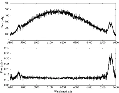
Quiescent LMXBs present emission line profiles quite similar to CVs: double-peaked hydrogen and helium lines, consistent with an accretion disc dominated profile. Luminous systems can show a range of different lines, the main ones being carbon, nitrogen, oxygen and silicon. In the optical, the strongest of these metal features is the Bowen blend (see McClintock et al. 1975, and Section 1.3), lines generated on the secondary surface via fluorescence. Figure 1.14 shows an example of a LMXB spectrum indicating the position of the Bowen blend. In quiescence, higher excitation lines of He II are absent, and only weak He I and H I are present in emission. If the disc is dim enough, the companion star spectrum emerges, facilitating radial velocity constraints and hence, the derivation of the system parameters.

1.3 Ca II and the Bowen blend

(42)

sys-24 CHAPTER 1. INTRODUCTION

4400 4500 4600 4700 4800 4900 5000 5100

Wavelength ( ˚A)

25 30 35 40 45 50

Flux

(mJy)

Bo

wen _HeII

Figure 1.14: Section of the MagE spectrum of the LMXB Sco-X1 showing the position of the Bowen blend and He II 4685.78Å.

(43)

[image:43.595.212.451.117.380.2]

1.3. CA II AND THE BOWEN BLEND 25

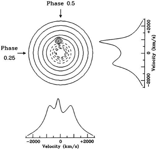
Figure 1.15: Trailed spectra of the Bowen blend and He II of Sco X-1 from Steeghs & Casares (2002).

features in 75% of these systems.

In the case of persistent LMXB systems, where no quiescent state is observed, as the spec-tra is dominated by the disc, we must look for a different source of radial velocity information. Steeghs & Casares (2002) proposed a new approach after finding narrow emission components, moving in anti phase with the disc components, in the Bowen blend (a mixture of mainly C III 4647.42/4650.25Å - N III 4640.64/4634.12Å lines). The idea that this feature was generated by the Bowen fluorescence process was proposed by McClintock et al. (1975), naming Sco X-1 and Her X-1 as good LMXB candidates to search for these lines. Looking at the trailed spectra of Sco X-1 by Steeghs & Casares shown in figure 1.15, we can see these narrow components trace the veloc-ity of the secondary star. The major caveat here is that these emission lines originate from the irradiated inner face of the donor star, and so their centre of light would not coincide with the centre of mass of the secondary, thus theKemvalue derived from this method is a lower limit to the true value ofK2and must be corrected to derive the true value. We will discuss this technique

(44)

1.4 Summary and Outline

We have presented a short review on the formation of spectral lines, mentioning the main fea-tures of CB classes. We have set the scene of CBs by showing their geometry, parameters, classifi-cation and evolution. We have also explained the importance of constraining orbital parameters other than just the orbital period to test evolution theories and determine the nature of CBs. We showed some of the main problems in constraining the dynamical parameters of persistent LMWBs and short period CVs. Finally, we introduced the Ca II triplet and the Bowen blend as suitable alternatives to constrain these parameters

(45)

Two

Methods

‘Understanding the light is a prerequisite to understanding the Universe’.

The Doppler tomography methods presented in this Section were published in:

“Emission line tomography of the short period cataclysmic variables CC Scl and V2051 Oph”

P. Longa-Pena; D. Steeghs; T. Marsh

Monthly Notices of the Royal Astronomical Society 2014, 447 (3): p 149-159

In this thesis, our main observational input has been time resolved spectroscopic data. Most of this time was spent developing and testing indirect imaging dependant methods to ob-tain a good estimate of the mass ratio of short period CVs with reliable uncerob-tainties. The func-tionality of the methods was extensively tested in several different lines of several systems, prov-ing to be reliable in the cases where there were known parameters. In practise, for non-eclipsprov-ing systems, obtaining a reliable estimate of any orbital parameter (except the orbital period) is not trivial, hence the importance of these new methods.

This chapter covers the basics of spectroscopy, CCD reduction and analysis of spectro-scopic data. We will describe the different methods used to analyse these data and the tech-niques used to constrain the system parameters for our CBs sample.

2.1 Spectroscopy

In astronomy, spectroscopy is the study of the electromagnetic radiation as a function of wave-length of a celestial body. It detects the absorption or emission of radiation within a continuum at certain energies, and relates these with the energy levels implied for a given quantum transi-tion. It is one of the most important tools for an astronomer to study the Universe. By means of studying the continuum and the emission and absorption lines, we can determine physical and chemical properties of distant celestial bodies.

(46)

28 CHAPTER 2. METHODS

In this Section we will discuss long-slit and Echelle spectroscopy, with special emphasis in the Magellan Echellette (MagE) spectrograph, with which most of the data in this thesis was obtained. In Section 2.1.3 we will discuss some basics of CCD reduction with special focus on MagE’s reduction pipeline.

2.1.1 Long Slit Spectroscopy

Although modern spectrographs are more diverse and complex than the original prism used to disperse light from the Sun, the basic elements are still the same for every astronomical spec-trograph. Every functional spectrograph should contain four essential elements (Carrol & Ostlie, 2007):

• a slit, to focus the light from the telescope and control the resolution. • a collimator, to parallelize the light beam.

• a disperser, to disperse incoming light from an astronomical source. • a camera, to focus the spectrum onto the detector.

As shown in Figure 2.1 the slit is placed in the focal plane of the telescope and the light from the star is focused onto the slit. Light then passes through a collimator, that forces the light to travel in a parallel direction and directs the beam towards the disperser, in most cases a grating with a number of grooves per millimetre. The dispersion of the grating depends directly upon the projected number of grooves per millimetre and is governed by the grating equation (Massey & Hanson, 2013):

mλ=σ(sin(i)+sin(θ)), (2.1) wherei is the incidence angle, θ is the refraction angle (see Figure 2.1), and m is an integer representing the order in which the grating is being used. Due to constructive interference, light from more than one order is simultaneously observed. The dispersion of an orderm, also known as the angular spread, can be found by differentiating:

dθ

dλ=

m

σcos(θ), (2.2)

for a given incidence anglei. Ifi=θ(called the Littrow condition):

dθ

dλ=

µ

2 λ

¶

tan(θ) (2.3)

(47)

2.1. SPECTROSCOPY 29

Figure 2.1: Schematic of the essential components of a spectrograph. Based on Figure 1 of Massey & Hanson (2013).

The spectral resolution is defined as:

R= λ

∆λ, (2.4)

where∆λis the difference between two, equally strong, lines than can be resolved (the width of one resolution element). This is called the resolution element.R∼1000 is considered a moderate resolution, while a resolution on the order ofR∼10000 is considered high. Most of our data is obtained atR∼4100.

2.1.2 Echelle spectroscopy

In the case of Echelle spectroscopes, a second dispersion element is inserted into the beam af-ter the diffraction grating to provide cross-dispersion of the light, spreading the various orders across the detector. An example of this is shown in Figure 2.2, a spectrum taken with the Magel-lan Echellette spectrograph, where the detector shows multiple orders next to each other, max-imising the use of the CCD detector.

For a given incidence angleθ, the free spectral rangeδλis the difference between two wavelengthsλmandλ(m+1)in successive orders:

δλ=λm−λ(m+1)=λ(m+1)

m

The angular spread,δθ, of a single echelle order will therefore be δλ_dd_λθ. Using equation 2.3 for the angular dispersion:

λ

σcosθ =δλ(2/λ) tanθ, (2.5) so the wavelength coverage of a single order will be:

δλ= λ

2

(48)

Figure 2.2: MagE spectra of the X-ray binary Sco X-1. The order numbers observed are 6 to 19 from top to bottom of the image, respectively, while the wavelength increases from bottom to top as shown in the figure.

The angular spread of a single order will be:

∆θ= λ

σcosθ. (2.7)

The above implies that the number of angstroms covered in a single order increases with the square of the wavelength (Equation 2.6), while the spatial length of each order increases linearly with each order (Equation 2.7). In Figure 2.2 we can see this effect, as the shorter wave-lengths span less of the chip and viceversa.

MagE Spectrograph

The Magellan Echellette (MagE) is located on the Magellan II (Clay) telescope at Las Campanas Observatory, Chile. MagE is a single object optical Echellette spectrograph. It provides spectral coverage from 3200 Å to 10000 Å in a single exposure, with a moderate resolution (R∼1000 to

R∼8000 ), achievingR=4100 (22 km/s pixel) with a 1” slit (Marshall et al., 2008).

Figure 2.4 shows the optical design of the instrument. Some elements are easily identified from the schematic of Figure 2.1 (the slit, collimator, prism, grating, camera and the detector). The light is focused onto a slit and then collimated by a mirror. There are also two cross dispers-ing prisms. The first one is used in double pass mode and the second one in a sdispers-ingle pass. The grating has 175 lines/mm and is used in a quasi-Littrow configuration.

(49)

2.1. SPECTROSCOPY 31

Figure 2.3: Photograph of MagE installed on the Magellan II telescope.

(50)

Figure 2.5: MagE bias frame. We can see some structure under the noise. A bias correction will remove this underlying structure from the final frames.

The detector is a 2048x1024 pixels CCD with 13.5µpixels, placed at the prime focus of a vacuum Schmidt camera.

The instrument itself is easy to operate, but presents challenges in the data reduction. To overcome the difficulties of flat-fielding over a very large wavelength range, a combination of focused and de-focused xenon (Xe) lamps are utilised to provide enough flux in the near ultra-violet, and quartz lamps are used for the red. Another remarkable challenge is the curving of the orders on the detector, as can be seen from Figure 2.2. This means that the spectral features are also tilted, with a different inclination along each order. This makes the sky subtraction partic-ularly difficult, since when the order is flattened, the sky line may be not perpendicular to the continuum, hence is not removed from the final spectra. We will discuss in more detail the data reduction of MagE spectra in the following section.

2.1.3 Data Reduction

A large portion of this work was carried out with MagE observations. The data were reduced with thePythonbased pipeline created by Dan Kelson (from the Carnegie Observatories Software Repository). Here we will discuss the basic reduction steps applicable to general spectrographs and remark upon the MagE pipeline specifics.

CCD Reduction