Group lending without joint liability

Original citation:

de Quidt, Jonathan, Fetzer, Thiemo and Ghatak, Maitreesh. (2016) Group lending without joint liability. Journal of Development Economics, 121 . pp. 217-236.

Permanent WRAP URL:

http://wrap.warwick.ac.uk/83246

Copyright and reuse:

The Warwick Research Archive Portal (WRAP) makes this work by researchers of the University of Warwick available open access under the following conditions. Copyright © and all moral rights to the version of the paper presented here belong to the individual author(s) and/or other copyright owners. To the extent reasonable and practicable the material made available in WRAP has been checked for eligibility before being made available.

Copies of full items can be used for personal research or study, educational, or not-for-profit purposes without prior permission or charge. Provided that the authors, title and full bibliographic details are credited, a hyperlink and/or URL is given for the original metadata page and the content is not changed in any way.

Publisher’s statement:

© 2016, Elsevier. Licensed under the Creative Commons Attribution-NonCommercial-NoDerivatives 4.0 International http://creativecommons.org/licenses/by-nc-nd/4.0/

A note on versions:

The version presented here may differ from the published version or, version of record, if you wish to cite this item you are advised to consult the publisher’s version. Please see the ‘permanent WRAP URL’ above for details on accessing the published version and note that access may require a subscription.

Group Lending Without Joint Liability

Jonathan de Quidt

Thiemo Fetzer

Maitreesh Ghatak

September 29, 2014

Abstract

This paper contrasts individual liability lending with and without groups to joint liability lending. We are motivated by an apparent shift away from the use of joint liability by microfinance institutions, combined with recent evidence that a) converting joint liability groups to individual liability groups did not a↵ect repayment rates, and b) an intervention that increased social capital in individual liability borrowing groups led to improved repayment performance. First, we show that individual lending with or without groups may constitute a welfare improvement over joint liability, so long as borrowers have sufficient social capital to sustain mutual insurance. Second, we explore how the lender’s lower transaction costs in group lending can encourage insurance by reducing the amount borrowers have to pay to bail one another out. Third, we discuss how group meetings might encourage insurance, either by increasing the incentive to invest in social capital, or because the time spent in meetings can facilitate setting up insurance arrangements. Finally, we perform a simple simulation exercise, evaluating quantitatively the welfare impacts of alternative forms of lending and how they relate to social capital.

Keywords: micro finance; group lending; joint liability; mutual insurance

1

Introduction

While joint liability lending by microfinance institutions (MFIs) continues to attract atten-tion as a key vehicle of lending to the poor, recently some MFIs have moved away from

⇤_{IIES, Stockholm University. Contact: [email protected].}

†_{STICERD and the Department of Economics, London School of Economics, Houghton Street, London,}

explicit joint liability towards individual lending. The most prominent such institutions are Grameen Bank of Bangladesh and BancoSol of Bolivia.1 _{However, interestingly, Grameen} and other such MFIs who have made this shift have chosen to retain the regular group meetings that traditionally went hand-in-hand with joint liability lending.

It is not clear what are the factors actually driving this trend, to the exent it exists.2 Nevertheless, these phenomena raise the question of the costs and benefits of using joint liability, and the choice between group loans with and without (explicit) joint liability. The existing literature, in general, has focused more on the benefits of joint liability. Besley and Coate (1995) is an early exception, showing that while joint liability can increase repayment rates by inducing borrowers to insure one another (repaying on behalf of their unsuccessful partners), there are also states of the world where a borrower who is expected to repay her partner’s loan may instead default, even though she would be willing and able to pay back her own loan. Using a limited enforcement or “ex-post moral hazard” framework introduced in the group lending context by Besley and Coate (1995), in this paper we study several issues raised by this apparent shift.

Our analysis is motivated by evidence from Gin´e and Karlan (2014) who find that ran-domly converting joint liability groups to individual liability at a Philippines MFI had no e↵ect on average repayment rates. We analyze how by leveraging the social capital of borrow-ers, individual liability lending (henceforth, IL) can mimic or even improve on the insurance arrangement reached under explicit joint liability (EJ), increasing repayment and borrower welfare. When this occurs, we term it “implicit joint liability” (IJ). Intuitively, in those states of the world where a borrower is able to repay her own loan but not that of her partner, IJ allows her to do this, yet in states of the world where she could repay her partner’s loan, social capital is leveraged to encourage her to do so. EJ does not permit such flexibility. The model has subtle implications for contract choice. From the existing literature, the general impression is that all else equal, more social capital increases the advantage of explicit joint liability relative to individual liability, such that individual liability is optimal for low social capital and joint liability for high social capital. We show that the relationship is not so straightforward. For low social capital, individual liability is still preferred, for intermediate

1_{For a discussion of the reasons for the shift in Grameen Bank’s lending strategy, see Muhammad Yunus’s}

article “Grameen Bank II: Lessons Learnt Over Quarter of A Century,” athttp://www.grameen.com/index. php?option=com_content&task=view&id=30&Itemid=0, accessed 18 December 2012.

2_{In a companion paper (de Quidt et al., 2013), we present data from the MIX Market suggesting a modest}

levels of social capital, explicit joint liability is preferred, but for high social capital individ-ual liability can once again dominate, due to its ability to induce welfare-improving implicit joint liability.

Since the previous argument does not rely on borrowing groups (though we believe im-plicit joint liability is likely to be easier in a group context), we next introduce a purely operational argument for group lending under IL. Group lending can reduce the lender’s transactions costs, shifting the time burden to the borrowers. This is valuable because it en-ables the lender to cut interest rates, relaxing the borrowers’ repayment incentive constraints, thus increasing repayment and welfare.

Finally, we consider evidence from Feigenberg et al. (2013), who find that an increase in the meeting frequency of individual liability borrowing groups created social capital, which led to a subsequent improvement in repayment rates. We discuss two mechanisms by which group meetings could create social capital or foster mutual insurance. First, because the more time borrowers spend together in groups, the more incentive they have to invest in social capital. Second, because maintaining an insurance arrangement requires spending time together, so group meetings can serve the dual purpose of repayment and insurance. Both mechanisms suggest that increasing meeting length or frequency could lead to more mutual insurance, however if borrowers are able to coordinate among themselves to spend time together, independent of the lender, artificially increasing meeting length or frequency with the aim of fostering insurance cannot increase welfare. In other words, an additional friction is required for the intervention of Feigenberg et al. (2013) to be welfare-improving.

Without any concrete evidence we can only speculate about what our theory implies about the apparent shift away from EJ to IL. The first part of our argument suggests that switching from EJ to IL can increase repayment rates if borrowers have sufficient social cap-ital. This prediction is consistent with the evidence from Gin´e and Karlan (2014). Although the average e↵ect on repayment of conversion to individual liability was zero, interestingly, repayment improved among borrowers with strong social ties, and deteriorated among bor-rowers with weak social ties, consistent with our theory.3 _{The third part of our argument} suggests that the creation of social capital through EJ may have paved the path for IJ in some cases, to the extent it became the more efficient lending arrangement.

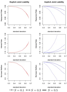
Finally, we carry out some simple simulation exercises using empirically estimated param-eters. The goal is to complement the theoretical analysis and to get a quantitative sense of the welfare e↵ects as well as the relevant parameter thresholds that determine which lending

3_{See Gin´e and Karlan (2014), table 8. This suggests that the joint distributions of social capital and}

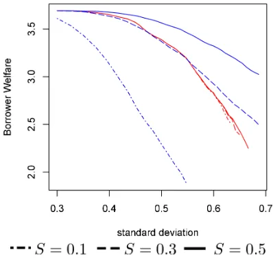
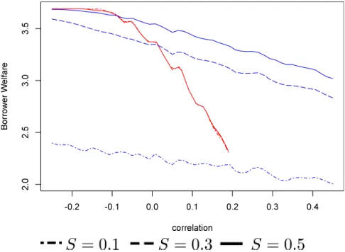
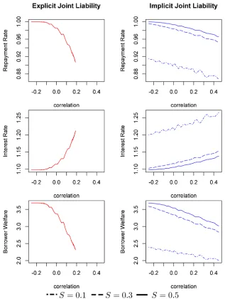
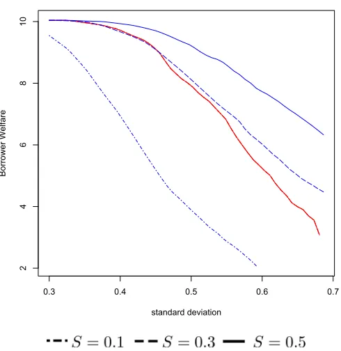
method is preferred. Our key findings are as follows. First, in low social capital environ-ments, EJ does well compared to IJ. For example, at our benchmark parameter values, when social capital is worth 10% of the loan size, the welfare attainable under IJ is 32.4% lower than that under EJ. However, with social capital worth 50% of the loan size, the welfare attainable under EJ is 5% lower than under IJ, and the advantage of IJ grows as the variance of borrower income increases. Second, we find that the interest rate, repayment rate and borrower welfare are all insensitive to social capital under EJ, whereas in the case of IJ, they are all highly sensitive. This is what we would expect, since EJ leverages both social capital and joint liability, while IJ leverages only social capital. To illustrate, under our benchmark parameter values, an increase in social capital from 10% of the loan size to 50% of the loan size increases borrower welfare under IJ by around 50%, while the e↵ect is negligible under EJ. When borrower incomes are uncorrelated, the insensitivity of EJ to the level of social capital suggests that it is a fairly robust contracting tool across lending contexts. However, when borrower incomes are positively correlated the advantage of EJ disappears. Intuitively, EJ requires groups to either all repay or all default. When incomes are positively correlated it is common to have multiple project failures, and since bailing all of them out is hard, the whole group defaults. IJ is robust to such states of the world because it does not require the whole group to repay.4

Although the model highlights the potential costs of EJ, it is premature to write o↵

EJ as a valuable contractual tool. Thus far we have one high quality randomized study of contractual form (Gin´e and Karlan, 2014) in which EJ seems not to play an important role. However in our theoretical analysis there are always parameter regions over which EJ is the most efficient of the simple contracts we analyze. A recent randomized control trial by Attanasio et al. (2011) finds stronger consumption and business creation impacts under EJ (albeit no significant di↵erence in repayment rates - note that in their context mandatory group meetings are not used under either IL or EJ). Carpena et al. (2010) analyze an episode in which a lender switched from IL to EJ and found a significant improvement in repayment performance. For the same reasons, Banerjee (2012) stresses the need for more empirical work in the vein of Gin´e and Karlan (2014) before concluding that EJ is no longer relevant. It is instructive to briefly look at the types of contracts currently used by MFIs. Cull et al. (2009) find that around two thirds of the MFIs in their sample (drawn from the MIX Market) predominantly use solidarity group loans (see footnote 2 above) or village banking, while around one third use individual lending; we find similar figures in de Quidt et al. (2013). Our concept of IJ is relevant to the “individual” category; the MIX Market notes that “loans based on consideration of the sole borrower, but disbursed through and

recollected from group mechanisms, are still considered individual loans.” A notable example is the Indian MFI Bandhan, which is one of the top MFIs in India, and is listed as having 3.6m outstanding loans in 2011. Bandhan does not use joint liability but disburses the majority of its loans through borrowing groups. Unfortunately, we do not have data on the method of disbursement of the sample of loans classified as individual, but we believe that many institutions are indeed using groups to disburse individual loans.

Much of the existing theoretical work has sought to characterize conditions under which explicit joint liability can lead to efficiency gains compared to traditional individual liability loans (see Ghatak and Guinnane (1999) for a review) by relaxing the underlying incentive or self-selection constraints. Since most of the literature assumed competitive lenders, the benefits of these gains are passed on to borrowers via relaxation of borrowing constraints, and/or lower interest rates. A key mechanism that is used to explain persistence of poverty in development economics has at its centre credit market imperfections, which are caused by informational and institutional frictions. While these can to some degree be mitigated by the use of collateral, by definition the poor do not have much in the way of collateralizable wealth. Therefore, they are likely to be credit constrained, thereby leading to a vicious cycle. A lot of the attention attracted by microfinance is because of its potential ability to tap into the information and enforcement advantages of the social networks the borrowers belong to, and harness it via joint liability to relax borrowing constraints. The literature has rationalized group lending starting with alternative types of credit market frictions–adverse selection, ex ante moral hazard, and ex post moral hazard or costly state verification–by highlighting the role of joint liability in generating peer selection, peer monitoring, and peer pressure. One of the broad theoretical points that emerge from the existing literature is that joint-liability loans are not always feasible, or even if they are, are not always efficient relative to individual-liability loans. Therefore, the fact that joint liability has both costs and benefits has always been implicit in the literature, but the focus mainly has been on mechanisms that harness the benefits. The model of Besley and Coate (1995), which is closest to ours in terms of the underlying credit market friction of ex post moral hazard, is an exception. It shows that joint liability gives borrowers an incentive to repay on behalf of their partner when the partner is unable to repay her own loan. If borrowers can threaten social sanctions against one another, this e↵ect is strengthened further. However, there are two problems with EJ. Firstly, since repaying on behalf of a partner will be costly, incentive compatibility requires the lender to use large sanctions and/or charge lower interest rates, relative to individual liability.5 _{Secondly, when a borrower is unsuccessful, sometimes EJ induces the successful}

5_{This issue is the focus of the analysis in Rai and Sj¨ostr¨om (2010). Because of this, de Quidt et al. (2013)}

partner to bail them out, but sometimes it has a perverse e↵ect, inducing them to default completely, while under IL they would have repaid. Rai and Sj¨ostr¨om (2004) and Bhole and Ogden (2010) approach these issues from a mechanism design perspective - designing cross-reporting mechanisms or stochastic dynamic incentives that minimize the sanctions used by the lender. Baland et al. (2013) provide an alternative explanation of the apparent trend away from what we call EJ towards IL, based on loan size. They find that the largest loan o↵ered under IL cannot be supported under joint liability, and for borrowers with access to both types of lending arrangements, the benefits from the latter are increasing in borrower wealth. We do not focus on this angle but briefly touch on the issue of loan size in section 2.5. Allen (2014) shows how partial EJ, whereby borrowers are liable only for a fraction of their partner’s repayment, can improve repayment performance by optimally trading o↵

risk-sharing with the perverse e↵ect on strategic default. We focus on how simple individual liability lending with no joint liability can achieve these e↵ects, as side-contracting by the borrowers can substitute for the lender’s enforcement mechanism.

Our model is also related to Rai and Sj¨ostr¨om (2010). In that paper, borrowers are as-sumed to have enough social capital to support incentive-compatible loan guarantees through a side-contract, provided they have sufficient information to enforce such side contracts. The role of groups is to provide publicly observable repayment so as to enable efficient side-contracting. In contrast, in our setting, repayment behavior is common knowledge among the borrowers, and it is the amount of social capital that is key. Groups play a role that depends on meeting costs and time use introduced in the next two sections.6

Other than the above mentioned papers, our paper is also broadly related to the the-oretical literature in microfinance that has emerged in the light of the Grameen Bank of Bangladesh abandoning explicit joint liability and switching to the Grameen II model, focus-ing on aspects other than joint liability, such as sequential lendfocus-ing (e.g., Chowdhury, 2005), frequent repayment (Jain and Mansuri, 2003; Fischer and Ghatak, 2010), exploring more general mechanisms than joint liability (e.g., La↵ont and Rey, 2003), and exploring market and general equilibrium (Ahlin and Jiang, 2008; McIntosh and Wydick, 2005; de Quidt et al., 2013).

The paper is structured as follows: in section 2 we present the basic model where in principle lending may take place with or without group meetings. We introduce our concept of implicit joint liability and show when it will occur and be welfare improving. Section 3

the lender must typically charge lower interest rates under EJ.

6_{Furthermore, in our model, borrowers are better o↵when they guarantee one another as their probability}

formalizes a key transaction cost in group and individual lending - the time spent attending repayment meetings. Section 4 then shows how meeting costs can give borrowers incentives to invest in social capital. Section 5 presents results of a simulation of the core model, and section 6 summarizes the results and concludes.

2

Model

We model a lending environment characterized by costly state verification and limited liabil-ity. Borrowers are risk neutral, have zero outside option, no savings technology and limited liability. They have access to a stochastic production technology that requires 1 unit of cap-ital per period with expected output ¯R, and therefore must borrow 1 per period to invest. There are three possible output realizations, R _{2 {}Rh, Rm,0}, Rh Rm > 0 which occur with positive probabilities ph, pm and 1 ph pm respectively. We define the following:

p_⌘ph+pm

4 ⌘ph pm

¯

R⌘phRh+pmRm.

We will refer to pas the probability of “success”, and ¯R as expected output.

We assume that output is not observable to the lender and hence the only relevant state variable from his perspective is whether or not a loan is repaid. Since output is non-contractible, the lender uses dynamic repayment incentives, as in Bolton and Scharfstein (1990). We assume that if a borrower’s loan contract is terminated following a default, she can never borrow again. Under individual liability (IL), a borrower’s contract is renewed if she repays and terminated otherwise. Under explicit joint liability (EJ), both contracts are renewed if and only if both loans are repaid.7

We assume that pairs of individuals in the village share some pair-specific social capital

7_{The assumptions of no savings, permanent exclusion and simple contracts are fairly standard in this}

worth S in discounted lifetime utility, that either can credibly threaten to destroy. In other words, a friendship yields lifetime utilityS to each person. If the social capital is destroyed it is lost forever. We assume that each individual has a very large number of friends, each worth S. Thus each friendship that breaks up represents a loss of size S. We discuss microfoundations for S in section 2.4 below.

We assume a single lender with opportunity cost of funds equal to ⇢ > 1. In the first period, the lender enters the community, observesSand commits to a contract to all potential borrowers. The contract specifies a gross interest rate,r and EJ or IL. We assume the lender to be a non-profit who o↵ers the borrower welfare maximizing contract, subject to a zero-profit constraint.8

In this section we ignore the role of groups altogether - being in a group or not has no e↵ect on the information or cost structure faced by borrowers and lenders. Although borrower output is unobservable to the lender, we assume it is observable to other borrowers. As a result, they are able to write informal side contracts to guarantee one another’s repayments, conditional on the output realizations. For simplicity, in the theoretical analysis we assume such arrangements are formed between pairs of borrowers.9

EJ borrowers will naturally side contract with their partner, with whom they are already bound by the EJ clause. Specifically, we assume that once the loan contract has been fixed, pairs of borrowers can agree a “repayment rule” which specifies each member’s repayment in each possible state Y _{2 {}Rh, Rm,0}⇥{Rh, Rm,0}. Then in each period, they observe the state and make their repayments in a simultaneous-move “repayment game”. Deviations from the agreed repayment rule are punished by a social sanction: destruction of S. The repayment rule, social sanction and liability structure of the borrowing contract thus deter-mine the payo↵s of the repayment game and beliefs about the other borrower’s strategy. To summarize, once the lender has entered and committed to the contract, the timings each period are:

1. Borrowers form pairs, and agree on a repayment rule.

2. Loans are disbursed, borrowers observe the state and simultaneously make repayments (the repayment game).

3. Conditional on repayments, contracts are renewed or terminated and social sanctions carried out.

8_{We abstract from other organizational issues related to non-profits, see e.g. Glaeser and Shleifer (2001).} 9_{This could be for example because there are two types of investment project available and returns within}

4. If an IL borrower’s partner was terminated but she repaid, she rematches with a new partner.

We restrict attention to repayment rules that are stationary (depending only on the state) and symmetric (do not depend on the identity of the borrower). This enables us to focus on the stationary value function of a representative borrower. Stationarity also rules out repayment rules that depend on repayment histories, such as reciprocal arrangements. In addition, we assume that the borrowers choose the repayment rule to maximize joint welfare. Welfare maximization implies that social sanctions are never used on the equilibrium path, since joint surplus would be increased by an alternative repayment rule that did not punish this specific deviation. In other words, although there may be many equilibria of the repayment game and associated social game as defined below: we focus on the welfare maximizing one.10

Given repayment probability ⇡, the lender’s profits are:

⇧=⇡r ⇢

and therefore the zero-profit interest rate is:

ˆ

r _⌘ ⇢

⇡. (1)

By symmetry, for interest rate r, each borroweripays ⇡r per period in expectation. There are two interesting cases that arise endogenously and determine the feasibility of borrowers guaranteeing one another’s loans. In Case A, Rm 2r and hence a successful borrower can always a↵ord to repay both loans. In Case B we haveRh 2r > Rm r, thus it is not feasible for a borrower with output Rm to repay both loans. Case B will turn out to be the more interesting case for our analysis, since in this case there is a cost to using joint liability lending. Specifically there are states of the world (when one borrower has zero output and the other hasRm) in which under joint liability both borrowers will default, since it is not feasible to repay both loans and they will therefore be punished whether or not the successful partner repays her loan. Meanwhile under individual liability, the successful partner is able to repay her loan and will not be punished if she does so.

Consider Case A. If borrowers agree to guarantee one another’s loans, they will repay in every state except (0,0), so the repayment probability is ⇡ = 1 (1 p)2 _{= p(2 p), in} which case ˆr = _p(2⇢_p). Therefore Case A applies if Rm _p(22⇢_p), i.e. when the successful

10_{A key implicit assumption is that borrowers cannot renegotiate on social sanctions, otherwise they would}

partner can a↵ord to repay both loans even if her income is onlyRm. If this condition does not hold, then it will not be feasible for the successful borrower to help her partner in this state of the world, and therefore Case B applies.

Definition 1 Case A applies when Rm _p(22⇢_p). Case B applies when Rm < _p(22⇢_p).

Suppose that borrowers only repay when both are successful, i.e. when both have at least Rm, which occurs with probability p2_{. If this is the equilibrium repayment rate, then} ˆ

r = _p⇢2. We make a simple parameter assumption that ensures that this will be the highest possible equilibrium interest rate (lowest possible repayment rate), by ensuring that even with income Rm, borrowers can a↵ord to repay _p⇢2.

Assumption 1 Rm _p⇢2.

We also assume thatRhis sufficiently large that a borrower withRhcould a↵ord to repay both loans even at interest rate ˆr= _p⇢2. Since this is the highest possible equilibrium interest rate, this implies thatRhis always sufficiently large for a borrower to repay both loans.

Assumption 2 Rh 2_p⇢2.

To summarize, together these assumptions guarantee that Rm r and Rh 2r on the equilibrium path.

We can now write down the value function V for the representative borrower, which represents the utility from access to credit. Suppose that borrower i’s loan is repaid with some probability ⇡. Since the repayment rule is assumed to maximize joint welfare, it follows that borrowers’s loans are only repaid when repayment leads to the loan contracts being renewed, and therefore the representative borrower’s contract is also renewed with probability ⇡. The lender charges an interest rate that yields zero expected profits, ˆr = _⇡⇢, so the borrower repays⇡ˆr=⇢ in expectation. Hence, (by stationarity) her welfare is:

V = ¯R ⇢+ ⇡V

= R¯ ⇢

1 ⇡. (2)

Provided IC1 is satisfied, borrower welfare is maximized by achieving the highest re-payment rate possible. To see this, suppose the lender charges some interest rate r. Then V = R₁¯ ⇡r_⇡. It can be verified that this is increasing in ⇡ if and only if IC1 holds. Therefore, since ⇡r = ⇢ in equilibrium, in the subsequent discussion the welfare ranking of contracts will be equivalent to the ranking in terms of the repayment probability.

Using (2) and ˆr= _⇡⇢ we can derive the equilibrium IC1 explicitly:

⇢  ⇡R.¯ (IC1)

By Assumption 1, the lowest possible equilibrium repayment probability⇡ is equal top2_. For the theoretical analysis we make the following parameter assumption that ensures IC1 is satisfied in equilibrium:

Assumption 3 p2_{R >¯ ⇢.}

Now that the model is set up we analyze the choice of contract type.

2.1

Individual Liability

Suppose first of all that the borrower does not reach a repayment guarantee arrangement with a partner. Since IC1 is satisfied, the borrower will repay her own loan whenever she is successful, so her repayment probability isp. Her utilityV is then equal to ₁R¯ ⇢_p.

Now we consider when pairs of IL borrowers will agree a repayment guarantee arrange-ment. If this occurs, we term it implicit joint liability (IJ). Note that at present borrowing groups are not required for this to take place.

Since IC1 holds, the borrowers want to agree on a repayment rule that maximizes their repayment probability. There are many possible such rules that can achieve the same re-payment rate, so for simplicity we focus on the most intuitive one: borrowers agree to repay their own loan whenever they are successful, and also repay their unsuccessful partner’s loan if possible.11

We already know that repayment of the borrower’s own loan is incentive compatible by IC1. For it to be incentive compatible for her to repay on behalf of her partner as well, it must be that social sanction outweighs the cost of the extra repayment, i.e. r  S. This gives us a constraint which we term IJ Incentive Constraint 2, or IJ IC2. For equilibrium

11_{An example of an alternative, less intuitive rule that can sometimes achieve the same repayment rate}

interest rate ˆr = _⇡⇢IJ IJ IC2 reduces to:

⇢_ ⇡IJ_{S. (IJ IC2)}

There is a threshold value ofS, ˆSIJ_{, such that IJ IC2 holds forS Sˆ}IJ_:

ˆ SkIJ ⌘

⇢ ⇡IJ

k

, k_2{A, B_},

wherekdenotes the relevant case. WhenS SˆIJ_{, it is feasible and incentive compatible for} borrowers to guarantee one another’s loans, and therefore they will do so as this increases the repayment probability and thus joint welfare. Therefore borrowers always engage in IJ ifS SˆIJ_.

Next we work out the equilibrium repayment probabilities and interest rates in cases A and B respectively. AssumeS SˆIJ_{. In Case A, a successful borrower can always a↵ord to} repay both loans, so both loans are repaid with probability ⇡IJ

A ⌘ 1 (1 p)2 = p(2 p).

In Case B, both loans are repaid whenever both are successful, and in states (Rh,0),(0, Rh). In state (Rm,0), borrower 1 cannot a↵ord to repay borrower 2’s loan, so she repays her own loan, while borrower 2 defaults and is replaced in the next period with a new partner. Therefore⇡IJ

B ⌘p2+ 2ph(1 p) +pm(1 p) =p+ph(1 p). Notice that both⇡IJA and ⇡IJB are greater thanp, the IL repayment probability.

The lender observes whether Case A or Case B applies, and the value of S in the com-munity, and o↵ers an individual liability contract at the appropriate zero profit interest rate. Equilibrium borrower welfare under individual liability is equal to:

VkIL(S) = 8 < : ¯

R ⇢

1 p S <Sˆ IJ k ¯

R ⇢

1 ⇡IJ

k S

ˆ SIJ

k

, k_2{A, B_}.

It is straightforward to see that asS switches from less than ˆSIJ

k to greater than or equal to it, VIL

k (S) goes up as ⇡IJk > p.

2.2

Explicit Joint Liability

she under individual liability, but she will default under joint liability because she is either unwilling or unable to repay both loans.

The borrowers will agree a repayment rule, just as under IJ. Since this will be chosen to maximize joint welfare, it will only ever involve either both loans being repaid or both defaulting, due to the joint liability clause that gives no incentive to repay only one loan. Subject to this, because IC1 holds, joint welfare is maximized by ensuring both loans are repaid as frequently as possible.

IC1 implies that when both borrowers are successful, they will both be willing to repay their own loans. We therefore need to consider i’s incentive to repay both loans when j is unsuccessful. Borrower i will be willing to make this loan guarantee payment provided the threat of termination of her contract, plus the social sanction for failing to do so, exceeds the cost of repaying two loans. Formally, this requires 2r  (VEJ _{+S). We refer to this} condition as EJ IC2. Rearranging, and substituting for ˆr = _⇡EJ⇢ , we obtain:

⇢  ⇡

EJ_{[ ¯R+ (1 ⇡}EJ_)S]

2 ⇡EJ . (EJ IC2)

We can derive a threshold, ˆSEJ_{, such that EJ IC2 is satisfied forS S}ˆEJ_:

ˆ

SkEJ ⌘max ⇢

0, ⇢ ⇡EJ

k

⇡EJ

k R¯ ⇢

⇡EJ

k (1 ⇡EJk )

, k2{A, B}

where as before,kdenotes the relevant Case.

Note that ˆSEJ _{can be equal to zero. This corresponds to the basic case in Besley and} Coate (1995) where borrowers can be induced to guarantee one another even without any social capital. This relies on the lender’s use of joint liability to give borrowers incentives to help one another, and is not possible under individual liability.

Provided S SˆEJ_{, borrowers are willing to guarantee one another’s repayments. The} repayment rule will then specify thati repays onj’s behalf wheneveri can a↵ord to and j is unsuccessful. If S <SˆEJ_{, borrowers will not guarantee one another. They will therefore} only repay when both are successful.

We now derive the equilibrium repayment probability under each Case. Firstly, if S < ˆ

SEJ_{, borrowers repay only when both are successful, so ⇡}EJ _=p2 _{in either Case.}

Now suppose S SˆEJ_{. In Case A, both loans can be repaid whenever at least one} borrower earns at least Rm. Thus the repayment probability is ⇡EJ

A = p(2 p). In Case B, Rm is not sufficient to repay both loans. Therefore both loans are repaid in all states except (0,0),(Rm,0),(0, Rm). In these three states both borrowers default. The repayment probability is therefore ⇡EJ

Borrower welfare is:

VkEJ(S) = 8 < :

¯

R ⇢

1 p2 S <Sˆ_kEJ ¯

R ⇢

1 ⇡EJ

k S

ˆ SEJ

k

, k_2{A, B_}.

Note that ˆSEJ

A  SˆBEJ. This is because the interest rate is lower in Case A, and V is higher (due to the higher renewal probability), so the threat of termination is more potent. Now that we have derived the equilibrium contracts assuming either IL or EJ, we turn to analyzing the lender’s choice of contractual form in equilibrium, which will depend crucially on the borrowers’ ability to guarantee one another’s loans.

Let us define V(S) _⌘ max_{VEJ_{(S), V}IL_{(S)} as the maximum borrower welfare from} access to credit. Observe that the repayment probability and borrower welfare from access to credit, V(S), are stepwise increasing in S.

2.3

Comparing contracts

In this section we compare borrower welfare under each contractual form. We have seen that EJ has the advantage that it may be able to induce borrowers to guarantee one another even when they have no social capital. However, in Case B it has a perverse e↵ect: in some states of the world borrowers will default when they would have repaid under IL.

This is most acute when pm > ph. Then⇡EJB =p+4(1 p)< p. Therefore in Case B, when4 0, EJ actually performs worse than IL for all levels of social capital - the perverse e↵ect dominates. Thus for Case B, when4 0, EJ would never be o↵ered.

We have already derived thresholds for S, ˆSIJ _{and ˆS}EJ_{, above which borrowers will} guarantee one another’s loans under individual and joint liability respectively. The lender’s choice of contract will depend on the borrowers ability to do so, so first we derive a lemma that orders these thresholds in Case A and Case B.

Lemma 1

1. SˆIJ

A >SˆAEJ.

2. Suppose ph pm. Then SˆBIJ >SˆBEJ.

Lemma 1 shows that supporting a loan guarantee arrangement requires more social cap-ital under IL than under EJ. The reason for this is that the lender’s sanction under EJ is a substitute for social capital in providing incentives to borrowers to guarantee one another.12 The lender is a non-profit who o↵ers the borrower welfare-maximizing contract. Therefore he o↵ers IL if VEJ_(S)VIL_{(S) and EJ otherwise. This will depend on the Case (A or B),} the sign of₄, and S. We summarize the key result of this section as:

Proposition 1 The contracts o↵ered in equilibrium are as follows:

Case A: IL is o↵ered at rˆ= ⇢_p for S <SˆEJ

A , EJ is o↵ered at r= ⇢ ⇡EJ

A , for S 2[ ˆS

EJ A ,SˆAIJ),

otherwise either EJ or IL are o↵ered at r = _⇡EJ⇢

A =

⇢ ⇡IJ

A (the lender is indi↵erent).

Case B, ₄ > 0: IL is o↵ered at rˆ = ⇢_p for S < SˆEJ

A , EJ is o↵ered at rˆ = ⇢ ⇡EJ

B for

S₂[ ˆSEJ

B ,SˆBIJ), IL is o↵ered at rˆ= _⇡⇢IJ

B for S

ˆ SIJ

B .

Case B, _{4 }0: IL is o↵ered at ˆr= ⇢_p for S <SˆIJ

B , IL is o↵ered at ˆr= ⇢ ⇡IJ

B otherwise.

Whenever EJ is o↵ered borrowers guarantee one another’s repayments. Whenever IL is o↵ered and S SˆIJ _{borrowers guarantee one another’s repayments.}

Proof. See appendix.

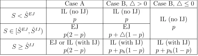
The result is summarized in Table 1, which gives the equilibrium contract and repayment probability ⇡ in alternate rows. Borrower welfare is not shown, but is easily computed as V = pR_{1 ⇡}⇢, and is strictly increasing in⇡.

Case A Case B, ₄>0 Case B,_{4 }0

S <SˆEJ IL (no IJ) IL (no IJ)

p p IL (no IJ)

S₂[ ˆSEJ_,SˆIJ₎ EJ EJ p

p(2 p) p+₄(1 p)

S SˆIJ EJ or IL (with IJ) IL (with IJ) IL (with IJ)

p(2 p) p+ph(1 p) p+ph(1 p)

Table 1: Equilibrium contracts and repayment probabilities

This table shows that there are clear trade-o↵s in the contractual choice. In Case A, IJ has no advantage over EJ because in both cases borrowers repay both loans whenever

12_{A slight complication arises in the proof because in Case B the repayment probability is higher under}

successful. In Case B when4 0, we have already remarked that EJ is always dominated by IL. Therefore basic IL is o↵ered for low S, and when S is high enough, borrowers will begin to guarantee one another, leading to an increase in the repayment rate and a fall in the equilibrium interest rate.

The most interesting case is Case B for 4 > 0. Here there is a clear progression as S increases. For low S, borrowers cannot guarantee one another under either contract, so basic IL is o↵ered. For intermediate S, EJ can sustain a loan guarantee arrangement but IL cannot, so EJ is o↵ered. Finally for highS, borrowers are able to guarantee one another under IL as well. Since this avoids the perverse e↵ect of EJ, the lender switches back to IL lending.

2.4

Microfoundations of social capital

So far we have treatedS as a “black box” as is common in the literature. While the primary goal of this paper is to demonstrate how social ties and social interactions can influence the credit market, it is worthwhile to consider conceptualizations of social capital that would be consistent with our setting.

We feel the most natural interpretation ofS is as the net present value of lifetime payo↵s in a repeated “social game” played alongside the borrowing relationship, similar to the multi-market contact literature, such as Spagnolo (1999), who models agents interacting simultaneously in a social and business context, using one to support cooperation in the other.

Suppose that each period, before loans are disbursed, each pair of friends plays the stage-game in Table 2 (presented in standard normal form), where s, c, d 0. Let S be the value of playing (C, C) indefinitely, i.e. S ⌘ s

1 . Ifdsthe stage-game has two Nash equilibria, (C, C) and (D, D). If d > s then only (D, D) is a stage-game equilibrium, but (C, C) can be sustained by trigger strategies in the repeated game ifd < s

1 , which we assume. When d _ s the stage-game is a coordination game, whereby players can coordinate on either equilibrium, while d > sis a standard prisoner’s dilemma. The fact that (D, D) is always an equilibrium is what enables people to credibly threaten to destroy S in response to a deviation, in this case to a deviation in either the social game or the repayment game.

C D

C s, s c, d

D d, c 0,0

We think of coordination games as a simple model of friendship. Individuals derive a utility benefit s from socializing with their friends, it is costly to extend friendship if it is not reciprocated (c 0), but it is not advantageous not to reciprocate (d < s). To us, this is the most natural way to think about social capital, essentially borrowers help one another in their borrowing a↵airs because something bigger is at stake, their social relationships.

The prisoner’s dilemma representation can represent, for example, a public goods game. Each partner contributes something to a public good, for example keeping the street in their neighborhood clean, keeping noise down, abiding by social norms, acting honestly in economic transactions. Each is tempted to deviate and not contribute (because d > s) but does so to preserve the continuation value S.

A third motivation is that perhaps borrowers have other insurance arrangements behind the scenes, and help one another in loan repayment to preserve those. For example, suppose that with probability⌧ a borrower su↵ers a non-monetary shockz, such as a health shock. One person in the village is especially well-positioned to assist with that (so the cost z is not incurred), at a cost to that person of c < z, provided they did not su↵er a shock themselves. For instance they could provide childcare, take the person to the hospital, take over their business for a day, and so on. Assume the setup is symmetric, then the expected per-period utility under a reciprocal arrangement to help one another is (1 ⌧)⌧c ⌧2_z. Without an arrangement, the utility is ⌧z, so the per-period gain from the agreement is ⌧(1 ⌧)(z c)>0 and the lifetime value isS _⌘ ⌧(1₁⌧)(z c). Suppose that individuals believe that a partner who has always helped in the past (when able) will always help in the future, but one who has ever deviated will never help again. Then it is clear that they will help when able if c < S provided the partner is expected to always help in the future. If the partner is not expected to help in the future, they too will not help today. This provides a stochastic foundation forS closely related to the social game outlined here.

cannot repay and the repayment meeting cannot be too long.

Second, lending can actually create temporary social capital (this bootstrap argument is very similar to the points made in Spagnolo, 1999). Supposed > S, so the only equilibrium in the repeated social game is (D, D) forever. However, suppose the individuals agree to guarantee one another’s loans, and to play (C, C) until someone deviates.13 _{Now, refusing to} repay the partner’s loan when required leads to a loss of social capital, this may be enough to sustain mutual insurance in the lending arrangement. Deviating in the social game also destroys social capital, and this renders mutual insurance in the repayment game impossible, leading to a decrease in the repayment rate and thus a fall inV. This additional cost may be sufficient to sustain cooperation in the social game.14 _{We choose not to emphasize this point} because we are primarily interested in social capital creation induced by the group structure rather than by lending itself.

Third, a comment on the friendship motivation. Throughout, we consider S to be the amount of social capital that can credibly be destroyed. One could think that with close friends or family members, the payo↵ structure is such that (D, D) is not an equilibrium, and for this reason destroying S is not a credible threat. Mutual insurance (based on such threats) may be less possible in these circumstances. This may be one motivation for why MFIs commonly restrict family members from joining the same joint liability groups.

Finally, throughout we assume that borrowers have a large number of friends (or, in the discussion of social capital creation, a large number of potential friends), and that after loss ofSwith one friend they can simply form a group with another. In many cases this may not be a plausible assumption. One could also think ofS as a reputation value that is lost once and for all. The “many friends” assumption is by no means crucial but it greatly simplifies the analysis, because it enables us to make the repayment problem stationary. Otherwise, loss of S would change the continuation value in the borrowing relationship as well as the social relationship.

2.5

A remark on loan size

For simplicity, our core model assumes loans of a fixed size. However, it is interesting to consider what happens as loan sizes grow.

13_{Note that by the assumption d > S the social capital created will be dissolved once the lending}

relationship ends, soS will be worth s

1 ⇡both <

s

1 where ⇡both is the probability that both loans are

repaid.

14_{This argument has one theoretically interesting implication. Suppose that if the lender charges a low}

interest rate r and o↵ers EJ, the joint liability penalty is enough to induce borrowers to guarantee one another. If the lender increases the interest rate tor0_{, they require social capital to achieve this. As a result,}

In our view, it is likely to be the case that efficient loan sizes, as determined by the production function, grow faster than social capital. For example, industrialization leads to increases in start-up costs relative to subsistence farming, while development may bring market or contract-based alternatives to social capital such as favor exchange, informal insurance or even, regretfully, traditional notions of friendship. Such developments imply a shift away from EJ and IJ, toward pure IL. To see this, note that the interest payment,r, is proportional to the loan size, so as loan sizes grow relative toS, the IC2 constraints tighten, decreasing the value of EJ. To the extent that groups are used to foster IJ (see below), it also implies a shift away from group lending.

Thus, our model is consistent with a stylized fact that can be seen in, for example, the well-known MIX Market microfinance dataset: loans disbursed to individuals tend to be larger than loans disbursed to groups. The model suggests a causal link from the loan size to the disbursement method.15

2.6

Discussion

Borrowers form partnerships that optimally leverage their social capital to maximize their joint repayment probability. Thus when social capital is sufficiently high to generate implicit joint liability, IL lending can dominate EJ: borrower i no longer defaults in state (Rm,0). This does not however mean there is no role for EJ. In particular, for intermediate levels of social capital, EJ can dominate IL - social capital is high enough for repayment guarantees under EJ but not under IL. We analyze borrower welfare under EJ and IL/IJ quantitatively in the simulations.

Let us compare our theoretical results with the findings of Gin´e and Karlan (2014), namely, average repayment does not change significantly when there is a random switch from EJ to IL. However, borrowers with stronger social ties are less likely to default relative to those with weaker social ties after switching to IL lending, and that these two e↵ects average out to zero.

If we look at Case A, Case B (4 > 0), and Case B (4  0), in all these three cases, for lowS, IL (no IJ) dominates EJ (though it should be noted that ˆSEJ _{could be negative} depending on parameter values, in which case calling this case that of “low S” would not make sense). We can see that in all these three cases, for high values of S (S SˆIJ_{), IJ} (weakly) dominates EJ. For Case A, they achieve the same repayment rate, but in the other two cases IJ achieves a strictly higher repayment rate. In contrast, with medium values ofS, EJ strictly dominates IL (no IJ) in Case A and Case B (₄>0), but not in Case B (_{4 }0).

15_{Baland et al. (2013) analyze this particular mechanism in detail, also relating loan sizes to borrower}

Therefore for “medium” levels of S, EJ is likely to dominate IL, unless the parameters of the distribution of returns are such that EJ is never desirable.

In the theoretical model, the optimal lending arrangment is always chosen. But in a randomized experiment, it is chosen randomly, including when it is not optimal. Clearly, Case B (4 0) is not consistent with either of the two findings of Gin´e and Karlan (2014). There, a random switch to IL should have raised repayment rates unconditionally. Case A is consistent with the average repayment rates being the same, but not the fact borrowers with stronger social ties are less likely to default relative to those with weaker social ties after switching to IL. Only Case B is consistent with both facts.

So far, we have ignored the use of groups for disbursal and repayment of loans. However, it is frequently argued (see e.g. Armend´ariz de Aghion and Morduch, 2010) that group meetings generate costs that di↵er from those under individual repayment. In the next section we show that this may induce the lender to prefer one or the other. We then proceed to show that by interacting with the benefits from social capital, group meetings may induce the creation of social capital. This is consistent with the results of a field experiment by Feigenberg et al. (2013).

3

Meeting Costs

In this section we lay out a simple model of loan repayment meeting costs. This immediately suggests a motivation for the use of groups. Holding group repayment meetings shifts the burden of meeting costs from the lender to the borrowers. This enables the lender to reduce the interest rate, which in turn makes it easier for borrowers to guarantee one another. Then in the next section we explore how the use of groups might create social capital, and thus generate implicit joint liability.

Since we want to focus on the interplay between meeting costs and social capital under individual liability, we assume that Case B applies and _{4 }0. Therefore we can ignore EJ and drop theA, B notation.

A common justification for the use of group meetings by lenders is that it minimizes transaction costs. Meeting with several borrowers simultaneously is less time-consuming than meeting with each individually. However, group meetings might be costly for the borrowers, as they take longer and are less convenient than individual meetings. We term IL lending to groups ILG and IL lending to individuals ILI.

borrowers and loan officers16_{Also, for simplicity, we assume that the cost of borrower time is} non-monetary so that borrowers are able to attend the meeting even if they have no income. However, more time spent in meetings by the loan officer increases monetary lending costs, for example because more sta↵must be hired.

Each meeting incurs a fixed and variable cost. The fixed cost includes travel to the meet-ing location (which we assume to be the same for borrower and loan officer for simplicity), setting up the meeting, any discussions or advice sessions that take place at the meeting, reminding borrowers of the MFI’s policies, and so on. This costs each borrower and the loan officer an amount of time worth f irrespective of the number of borrowers in the group. Secondly there is a variable cost that depends on the number of borrowers at the meeting. This time cost is worth _v per borrower in the meeting. This covers tasks that must be carried out once for each borrower: collecting and recording repayments and attendance, reporting back on productive activities, rounding up missing borrowers, and so on. As with the fixed cost, each borrower and the loan officer incurs the variable cost. We assume that for group loans, each borrower also has to incur the cost having to sit through the one-to-one discussion between the loan officer and the other borrower, i.e., in a two group setting, the total variable cost per borrower is 2 v whereas under individual lending, it is v.

Therefore, in a meeting with one borrower, the total cost incurred by the loan officer is

f+ v, and the total cost incurred by the borrower is the same, bringing the aggregate total time cost of the meeting to 2 f + 2 v. In a meeting with two borrowers the loan officer incurs a cost of f + 2 v, and similarly for the borrowers. Thus the aggregate cost in this case is 3 _f+ 6 _v. The lender’s cost of lending per loan under ILI is⇢+ _f+ _v. Under ILG it is ⇢+ f

2 + v. Therefore the corresponding zero-profit interest rates are ˆrILI ⌘

⇢+ f+ v

⇡

and ˆrILG ⌘ ⇢+

f

2 + v

⇡ .

Accounting for these costs, per-period expected utility for borrowers under ILI is ¯R ⇢ 2( f+ v). Under ILG, the per-period utility is ¯R ⇢ 32( f+ 2 v).17

Of course, the first thing to check is whether one lending method is less costly than the other in the absence of any loan guarantee arrangement between borrowers. This is covered by the following observation:

16_{This may not be too unrealistic. For example, the large Indian MFI, Bandhan, deliberately hires loan}

officers from the communities that they lend to.

17_{We need to adapt Assumptions 1, 2 and 3 to reflect the additional costs. We assumeRm} ⇢+12( f+2 v)

p2 ,

Rh 2

⇢+1 2( f+2 v)

Observation 1 Suppose S= 0. The lender uses ILG if and only if v<

f

2.18 The intuition is straightforward. When f

v is large, i.e., fixed costs are important relative

variable costs (e.g., when a large part of repayment meetings is repetitious) it is economical to hold group meetings. However, the more time is spent on individual concerns, the more costly it is to the borrowers to have to attend repayment meetings in groups because they have to sit through all the bilateral exchanges between another borrower and the loan officer. Microfinance loans are typically highly standardized and so f

v will be relatively large, which

is consistent with the common usage of group lending methods in microfinance.

Now consider borrowers’ incentives to guarantee one another’s loans. First we observe that for a given _v, _f, half of the aggregate meeting cost per borrower is borne by the lender under ILI, while only a third is borne by the lender under ILG. The lender passes on all costs through the interest rate, so inspecting the value functions suggests that it is innocuous upon whom the cost of meetings falls. In fact this is not the case. Consider once again IJ IC2: r S. The only benefit a borrower receives from bailing out her partner is the avoidance of a social sanction, while the cost depends on the interest payment she must make. Therefore a lending arrangement in which the lender bears a greater share of the costs, and thus must charge a higher interest rate, tightens IJ IC2. This gives us the next proposition, which is straightforward:

Proposition 2 Borrowers are more likely to engage in IJ under group lending than indi-vidual lending: SˆIJG _<SˆIJI_.19

The implication of this result is that there is a trade-o↵between minimizing total meeting costs, and minimizing those costs borne by the lender. It may actually not be optimal to minimize total costs as shown by the following corollary, the proof of which is straightforward and given in the appendix.

Corollary 1 Suppose S 2 [ ˆSIJG_,SˆIJI_{). Borrower welfare under ILG may be higher than}

under ILI, even if v >

f

2 .

It is worth pointing out that as in the earlier analysis of IJ, nothing in the results presented so far requires IL borrowers to form insurance arrangements with their own group members. In the next section we analyze the interaction between meeting costs, insurance initiation and social capital creation, which will more naturally lead to insurance arrangements forming within group boundaries.

18_{Proof: S = 0 implies IJ is not possible so ⇡ = p under ILI and ILG. The result then follows from}

comparison of per-period borrower welfare.

19_{Proof: Borrowers are willing to guarantee their partner’s repayments providedr S. Plugging in for}

the interest rates under ILG and ILI, we obtain ˆSIJG₌⇢+12( f+2 v)

<⇢+ f+ v

4

The role of groups

In this section we show how group lending can facilitate mutual insurance among borrowers where individual lending cannot. For example, groups may generate social capital that is then used to sustain IJ. The analysis is motivated by the findings of Feigenberg et al. (2013). In their experiment, borrowers who were randomly assigned to higher frequency repayment meetings went on to achieve higher repayment rates. The authors attribute this to social capital being created by frequent meetings, social capital which can then support mutual insurance.

We think there are two broad classes of mechanism by which meetings can increase repayment rates. The first is that forcing borrowers to interact frequently, the lender can increase their incentive to invest in social capital. Intuitively, the more time I spend with someone, the greater the benefit to forming a social bond with that person. This is our interpretation of the Feigenberg et al. (2013) findings. The second is that meetings play a more mechanical role in facilitating mutual insurance. This could be because borrowers need to observe one another’s outcomes or repayments, or play a message game as in Rai and Sj¨ostr¨om (2010). It could be that meetings help borrowers coordinate on mutual insurance which is too difficult to arrange independently.20

We model each of these in turn. On the first, we assume that investing in social capital is costly, such that borrowers do not do it independently. The situation we have in mind is that borrowers have some baseline level of social capital created in the normal run of life, but this is insufficient to sustain mutual insurance in borrowing without an extra incentive to create more. Borrowing groups increase the return to investment in social capital by providing an added benefit: social time spent with the partner. We also discuss informally under what conditions a simpler mechanism–spending time together automatically generates social capital–can have the same e↵ect.

Turning to the second, we assume that sustaining mutual insurance requires borrowers to spend a minimum amount of time with another borrower (their insurance partner) each period. This is perfectly possible under individual lending, but groups have an advantage in that the group meeting time can serve this purpose.

In both frameworks we discuss the welfare consequences of increasing the length of group meetings, which we treat as a simple proxy for the repayment frequency in Feigenberg et al.

20_{It could even be that without the group, borrowers would be less able to interact. Indeed, in some}

(2013). We take this approach because changing repayment frequency is non-trivial in our setup.21

4.1

Groups and social capital creation

Suppose that initially borrowers do not have any social capital, because creating social capital is too costly. For example, borrowers must invest time and e↵ort in getting to know and understand one another, extend trust that might not be reciprocated, and so forth. Assume that social capital can take two values only, 0 and S > 0 and for a pair to generate social capital worthS in utility terms, each must make a discrete non-monetary investment that costs them ⌘. In the absence of microfinance, they prefer not to do so, i.e., ⌘ > S. In the context of the discussion in section 2.4, ⌘ represents an up-front cost in initiating a friendship, favor exchange arrangement, etc.

Once lending is taking place, social capital generates an indirect benefit, by enabling the formation of a guarantee arrangement. This may or may not be sufficient to induce them to make the investment - that would depend on how ⌘ S compares with the insurance gains from microfinance. We also assume that group meetings confer an additional benefit, namely that spending time in a group meeting with a partner with whom one shares social capital is less arduous than with a stranger. Naturally this increases the incentive to invest in social capital when groups are used.

To make the point as simply as possible, we assume that the lender can observe whether borrowers have invested inSand adjust the interest rate accordingly to reflect the repayment probability. This of course increases the incentive to invest in S because that leads to an interest rate cut, however it greatly simplifies the analysis while preserving the main point.22 Suppose the lender o↵ers ILI and S would be sufficiently large to sustain IJ. If the borrowers prefer to invest in social capital, each time their partner defaults they must invest in social capital with their new partner. We obtain the following result:

Lemma 2 Borrowers invest in social capital under ILI if and only if:

⌘ S _G1. (3)

where

G1⌘ ph(1 p)

⇥_¯

R ⇢ 2( f+ v)

⇤

(1 p)(1 (p+₄(1 p))) .

21_{In a companion paper, Feigenberg et al. (2014) discuss a treatment that comes closer to our setup:}

increasing the meeting frequency without changing the repayment frequency.

22_{We thank a thoughtful referee for suggesting this approach. The working paper version of the paper}

The proof is given in the appendix. The greater the welfare gain from insurance, captured by the ratioph(1 p)/(1 p), the higher is G1 so the more likely the borrowers will invest in social capital.

Now assume that under ILG, the per-meeting cost to borrowers is decreasing in S. For simplicity, we assume that the cost to the borrowers of the time spent in group meetings is (1 (S))( f+ 2 v). In particular, (0) = 0 and (S) = >0. The larger is , the smaller the disutility of group meetings, and when >1, borrowers actually derive positive utility from group meetings that is increasing in the length of the meeting. We can now check when social capital will be created in groups.

Lemma 3 Borrowers invest in social capital under ILG if:

⌘ S _G2. (4)

where

G2_⌘ ph(1 p)

⇥_¯

R ⇢ 3₂( f + 2 v)

⇤

+ (1 p)( f+ 2 v)

(1 p)(1 (p+4(1 p))) .

The proof is given in the appendix. The greater the welfare gain from insurance, the higher is G2, but in addition, G2 is increasing in , which represents the reduction in the cost of attending group meetings when the borrowers have social capital. The larger is G2, the more likely borrowers are to invest in social capital.

Lemmas 2 and 3 suggest that there may exist an interval, (G1, G2] for⌘ S over which groups create social capital but individual borrowers do not. The condition for this to be the case is derived in the next proposition, which follows from straightforward comparison of (3) and (4):

Proposition 3 If the following condition holds:

> ph(1 p)( v

f

2) (1 p)( f + 2 v)

(5)

then there exists a non-empty interval for⌘ S over which both (3) and (4)are satisfied. If

⌘ S lies in this interval, groups create social capital, and individual lending does not.

Thus, when creating social capital sufficiently o↵sets the cost to borrowers of attending group meetings, borrowing groups may create social capital and guarantee one another’s loans, while individual borrowers may not do so. We can see that the threshold for in (5) is negative if f

2 > v and so the condition (5) is always satisfied if group lending has a cost advantage to the lender. Even if this is not the case, and v

f

is always strictly less than 1 and therefore, there always exists a high enough (but strictly less than 1) such that the condition (5) would hold. However it does not yet establish that the use of groups is necessarily welfare-improving. In other words, observing that groups are bonding and creating social capital does not tell the observer that group lending is the welfare-maximizing lending methodology. All it tells us is that investment is preferred to no investment under ILG, and no investment is preferred to investment under ILI. The welfare ranking of these two will depend on the meeting costs, ⌘ and S. The following proposition addresses the welfare question.

Proposition 4 Suppose condition (5) is satisfied and ⌘ S ₂ (G1, G2]. Borrower welfare under ILG is higher than that under ILI if:

⌘ S _G3 (6)

where

G3 _⌘ ph(1 p) ¯R ⇢ + 2(1 ⇡

IJ₎₍

f+ v) 12(1 p)( f+ 2 v)(3 2 )

(1 p)(1 (p+4(1 p))) .

The derivation simply compares welfare under ILI when borrowers do not invest to welfare under ILG when they do. G3 is higher the larger is the meeting cost under ILI relative to under ILG. It is also increasing in , representing the reduction in the cost of attending group meetings when the borrowers have social capital. (6) is always satisfied provided group meeting costs are low enough and is high enough.

We conclude this analysis with an observation that combines the above results. If meeting costs are lower under group lending then it dominates individual lending both from an efficiency and a social capital creation perspective.

Observation 2 Suppose >0 and total meeting costs per borrower are weakly lower under ILG than ILI, i.e. v 

f

2. Then G1 < G2< G3, i.e.:

1. There always exists an interval for ⌘ S over which groups create social capital and individuals do not.

2. Borrower welfare is weakly higher under ILG than ILI for all values of ⌘ S.

4.1.1 Meeting frequency and social capital creation

Now we take this basic framework and carry out one particular comparative-static exercise, motivated by the findings of Feigenberg et al. (2013). They find that groups that were randomly assigned to meet more frequently have better long-run repayment performance, which they attribute to higher social capital and informal insurance within the group. It is not possible to model repayment frequency in our simple setup, but nevertheless our model is able to capture some of this intuition.

We model an increase in meeting frequency as an increase in meeting costs, represented by an increase in either f or v. The more time spent in group meetings, the greater the benefit from social interaction within those meetings, captured by . Intuitively, it may not be too costly to attend meetings once a month with a stranger, but the more frequent those meetings are, the greater the incentive the borrowers have to build social capital.

However, more frequent meetings require more of the loan officer’s time as well, leading to higher lending costs and a higher interest rate. This reduces the borrowers’ incentive to invest inS, since the higher meeting costs reduce the value of maintaining access to credit. The net e↵ect on borrowers willingness to invest inS is positive if is sufficiently large, as shown by the following proposition.

Proposition 5 Increases in f or v make borrowers under group lending more willing to

invest in social capital if and only if the following condition holds:

> 3 ph(1 p)

2(1 p) . (7)

The proof is immediate from inspection of (4). This proposition suggests that an increase in meeting costs could actually be welfare-improving. Notice that the right hand side of (7) is strictly smaller than 3₂, and note too that if 3₂ then the utility of meeting with one’s partner more than o↵sets the welfare cost of time in meetings, such that increase in meeting time strictly increase borrower welfare.

However, under the more realistic assumption that < 3

choice. Feigenberg et al. (2013)’s intervention may not have been welfare improving.23 _To obtain a welfare increase, one must add a friction such as a coordination failure between borrowers (leading them to fail to invest optimally), or an externality. For example, if the lender’s break-even constraint is sufficiently tight that he must exit the market if borrowers do not mutually insure, but borrowers do not internalize this cost because there are many of them, interventions that push borrowers into investing in S could enable the lender to stay in business, increasing welfare.

Observation 3 Suppose < 3

2. Then increases in meeting costs are welfare decreasing,

even if they generate social capital creation and mutual insurance.

4.1.2 Mechanical social capital creation

An alternative possibility is that groups mechanically create social capital simply by spending time together. Perhaps surprisingly it turns out that this mechanism cannot sustain IJ. Suppose that each time a borrower obtains a new partner, automaticallySis created between them. Can they use this social capital to insure one another? The answer is no, as can be seen by considering their modified IJ IC2. If a borrower repays on behalf of her unsuccessful partner, she keeps her S at cost r. If she does not, she receives a new partner and new S next period. Thus her incentive constraint is (V +S) r (V +S) which cannot hold for positiver. Mutual insurance requires a cost to deviating. One way to restore this is to assume that it takes time for social capital to be generated, which decreases the right hand side of the condition (V is lower because mutual insurance is not possible until new S is generated). The analysis above can capture this mechanism in a simple reduced form way via the cost of social capital formation, ⌘.

4.1.3 Meetings lower the cost of investment

An alternative way to use our framework is as follows. Assume that there are no direct benefits to having social capital in group meetings ( = 0), but that group meetings lower the cost of investment in social capital or the cost of setting up mutual insurance (⌘ILG _<⌘ILI_). Then, naturally, group meetings will lead to more insurance.

23_{A thoughtful referee pointed out that their intervention (increasing meeting frequency) was temporary,}