warwick.ac.uk/lib-publications
Manuscript version: Published Version
The version presented in WRAP is the published version (Version of Record).
Persistent WRAP URL:
http://wrap.warwick.ac.uk/128477
How to cite:
The repository item page linked to above, will contain details on accessing citation guidance
from the publisher.
Copyright and reuse:
The Warwick Research Archive Portal (WRAP) makes this work by researchers of the
University of Warwick available open access under the following conditions.
Copyright © and all moral rights to the version of the paper presented here belong to the
individual author(s) and/or other copyright owners. To the extent reasonable and
practicable the material made available in WRAP has been checked for eligibility before
being made available.
Copies of full items can be used for personal research or study, educational, or not-for-profit
purposes without prior permission or charge. Provided that the authors, title and full
bibliographic details are credited, a hyperlink and/or URL is given for the original metadata
page and the content is not changed in any way.
Publisher’s statement:
Please refer to the repository item page, publisher’s statement section, for further
information.
On the control and suppression of the Rayleigh-Taylor
instability using electric fields
Radu Cimpeanu,1Demetrios T. Papageorgiou,1and Peter G. Petropoulos2
1Department of Mathematics, Imperial College London, SW7 2AZ London, United Kingdom
2Department of Mathematical Sciences, New Jersey Institute of Technology, Newark,
New Jersey 07102, USA
(Received 2 August 2013; accepted 29 January 2014; published online 19 February 2014)
It is shown theoretically that an electric field can be used to control and suppress the classical Rayleigh-Taylor instability found in stratified flows when a heavy fluid lies above lighter fluid. Dielectric fluids of arbitrary viscosities and densities are consid-ered and a theory is presented to show that a horizontal electric field (acting in the plane of the undisturbed liquid-liquid surface), causes growth rates and critical sta-bility wavenumbers to be reduced thus shifting the instasta-bility to longer wavelengths. This facilitates complete stabilization in a given finite domain above a critical value of the electric field strength. Direct numerical simulations based on the Navier-Stokes equations coupled to the electrostatic fields are carried out and the linear theory is used to critically evaluate the codes before computing into the fully nonlinear stage. Excellent agreement is found between theory and simulations, both in unstable cases that compare growth rates and in stable cases that compare frequencies of oscillation and damping rates. Computations in the fully nonlinear regime supporting finger formation and roll-up show that a weak electric field slows down finger growth and that there exists a critical value of the field strength, for a given system, above which complete stabilization can take place. The effectiveness of the stabilization is lost if the initial amplitude is large enough or if the field is switched on too late. We also present a numerical experiment that utilizes a simple on-off protocol for the electric field to produce sustained time periodic interfacial oscillations. It is suggested that such phenomena can be useful in inducing mixing. A physical centimeter-sized model consisting of stratified water and olive oil layers is shown to be within the realm of the stabilization mechanism for field strengths that are approximately 2×10⁴ V/m.
C
2014 AIP Publishing LLC. [http://dx.doi.org/10.1063/1.4865674]
I. INTRODUCTION
The stabilization of the Rayleigh-Taylor instability1–3 by external effects such as shear or transverse oscillations has been extensively considered both theoretically and experimentally. It has been shown4 that shear can stabilize the Rayleigh-Taylor instability in thin films by a nonlinear mechanism that appears to be quite general and can lead to complex spatiotemporal dynamics, while a more recent study5predicts a similar, albeit more dynamically complex, saturation for a thin film two-fluid system in a Couette device by transverse oscillations of one of the walls. Similar shear-induced stabilization of capillary instability in cylindrical geometries has also been described.6,7 The competition between gravitational and capillary instabilities has been studied8for a liquid film wetting the outer surface of a circular tube whose axis is horizontal (see also Ref.9); it is shown that time-periodic oscillations of the cylinder along its axis can stabilize the flow in the sense that the lobes that form in the absence of oscillations become longer and of smaller amplitude. Recent experimental studies10 of the development of the Rayleigh-Taylor instability in centimeter-sized geometries incorporate magnetic fields to produce precise and controlled initial perturbations. Most of the mechanisms outlined above require some form of mechanical actuation involving moving parts; our objective herein is to employ an electric field to achieve stabilization and, in particular, to
obtain controllable and tunable oscillatory two-fluid flows that can be useful in mixing in confined geometries.
We are interested in flows of immiscible stratified liquids in small scale geometries, where viscosity, surface tension, and gravity compete to select the dynamics. In particular, we focus on centimeter-sized domains appropriate to desktop experiments where electric fields can be easily applied; this provides a rich dynamical system that can be controlled passively or actively using the applied electric field whose direction relative to the plane of the interface influences electro-hydrodynamic instabilities. For example, it has been established in several pioneering works11–13 that a field which is perpendicular to the undisturbed interface induces instabilities that have found application in modern soft lithography.14,15 The control of such instabilities in a stably stratified air-gas system using feedback control has been demonstrated experimentally16in a circular device of radius 1.9 cm with a 3 mm thickness liquid layer wetting the bottom plate electrode and a 0.785 mm gas layer (sulfur hexafluoride to prevent dielectric breakdown) sandwiched between the liquid and top electrode. The spatiotemporally modulated electric field was selected to produce a stabilizing feedback force on the interface that undergoes electrohydrodynamic instabilities due to a constant background imposed field. If, however, the field is parallel to the interface (or parallel to the axis in cylindrical jet geometries), it induces a stabilizing effect. For example, it can prevent or delay rupture events in liquid sheets in the presence of van der Waals forces,17,18it can produce large am-plitude nonlinear traveling wave structures19and it can suppress the Kelvin-Helmholtz instability.20 In cylindrical geometries axial electric fields can suppress capillary instabilities in liquid jets and bridges as observed in several experiments.21–25In the context of the Rayleigh-Taylor instability such stabilization (allied to nonlinear aspects in the long wave limit) has been recently described26(see also the linear studies27,28). The physical mechanism responsible for this electrostatic stabilization is the modification of the normal stresses due to the presence of Maxwell stresses at the interface, that in turn affect the perturbation pressures in the vicinity of the interface. Details of the linear stability aspects of this mechanism are provided here in order to provide benchmarks capable of evaluating the accuracy of direct numerical simulations (DNS) and to obtain a quantitative understanding of incipient instabilities. With tested numerical tools at our disposal we then explore the nonlinear dynamics of the problem at arbitrary Reynolds numbers with emphasis placed on suppression of gravitational instabilities, when present, and establishment of temporal voltage protocols (essentially on-off systems for simplicity) that produce controlled time-periodic sustained interfacial oscillations that can be useful in mixing. The direct numerical simulations are carried out using the GERRIS29 platform, whose utility has been demonstrated on numerous occasions;30,31there is also a focus on efficient implementation of electric effects,32 which render it highly suitable in the context of our application.
The paper is structured as follows. SectionIIintroduces the governing equations and bound-ary/interfacial conditions for both the fluid dynamics and the electrostatics. SectionIIIis devoted to the general linear stability problem and an implicit dispersion relation is derived and used to charac-terize electrohydrodynamic stability properties. In Sec.IVthe linear theory is employed to validate the direct numerical simulation results for wide parameter ranges. Simulations are performed to probe the nonlinear regime in several directions including implementation of complete stabilization as well as demonstrating active control protocols that can produce sustained interfacial oscillations with mixing ramifications. In Sec.Vwe provide our conclusions.
II. MATHEMATICAL MODEL
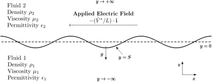
FIG. 1. Schematic of the problem with fluid 2 lying above fluid 1 and separated by the interfacey=S(x,t). A constant horizontal electric field of size ¯V∗/Lis applied horizontally as shown. (The direction of the field is unimportant.)
1,2, viscositiesμ1,2, densitiesρ1,2and the corresponding velocity vectors areu1,2=(u1,2, v1,2). We
denote the constant surface tension coefficient at the interface byσ. When the interface is flat (S= 0), the field is uniform and given byE0= −( ¯V∗/L)i, and when the interface is disturbed we need
to consider voltage potentialsV1,2in regions 1,2 that satisfy Laplace’s equation. This follows from
the electrostatic approximation: Maxwell’s equations reduce to∇ ×E1,2=0,∇ · (1,2E1,2)=0,
henceE1,2= −∇V1,2from the former condition, with Laplace equations following from the second
condition away from the interface:
∂2
∂x2 +
∂2
∂y2
V1,2=0. (1)
The dimensional momentum and continuity equations are
ρ1(u1t+(u1· ∇)u1)= −∇p1+μ1u1−ρ1gj, (2)
ρ2(u2t+(u2· ∇)u2)= −∇p2+μ2u2−ρ2gj, (3)
∇ ·u1,2=0, (4)
wherep1,2denote the pressures in each fluid andgis the acceleration due to gravity. Since the fluids
are perfect dielectrics with constant permittivities, there are no charges present hence the Lorentz force is absent in the momentum equations(2)and(3). However Maxwell stresses have jumps at the interface and this is accounted for in the normal stress balance(12).
We introduce the density and viscosity ratios
r=ρ1/ρ2, m=μ2/μ1, (5)
and non-dimensionalize using fluid 1 as reference. Lengths are scaled byL, velocities by a reference valueUand pressures byρ1U2; the following dimensionless parameters emerge
˜ g= g L
U2, μ˜ =
μ1
ρ1U L
, p =2
1
, We= σ
ρ1g L2
(6)
that represent an inverse square Froude number ˜g, an inverse Reynolds number ˜μ, the permittivity ratiop, and an inverse Weber number denoted byWeand which measures the ratio of surface tension
to gravitational forces. Furthermore, we scale voltage potentials byV∗ so that the dimensionless electric parameter measuring the size of Maxwell stresses in the interfacial stress balance equation becomes unity in fluid 1 variables. Inspection of the stress tensor(18)below, shows that this choice necessitates
ρ1U2=
1(V∗)2
L2 ⇒V
∗=U Lρ
As a result, the dimensionless boundary condition at the right of the domain x =1/2 becomes V1,2=V¯, where the dimensionless parameter ¯V =V¯∗/V∗ measures the magnitude of the applied
electric potential difference. The dimensionless Navier-Stokes equations become
˜
u1t+( ˜u1· ∇) ˜u1= −∇p˜1+μ˜ u˜1−g˜j, (8)
˜
u2t+( ˜u2· ∇) ˜u2= −r∇p˜2+mμ˜ru˜2−g˜j, (9)
∇ ·u˜1,2 =0, (10)
wherej=(0, 1) and tildes are used to refer to dimensionless quantities.
Since we assume a sharp interface (this is preferable in analytical treatments but is relaxed in the computational treatment as we will see below) electrohydrodynamic coupling and capillary effects occur through the interfacial boundary conditions. The conditions required aty=Sare a kinematic condition, and continuity of: normal and tangential stresses, velocities, normal components of the displacement field ˜E˜, and tangential components of the electric field (equivalently continuity of voltage potentials):
˜
vi =St+u˜iSx, i =1,2, (11)
[n·T ·n]12=σ κ,˜ (12)
[t·T ·n]12=0, (13)
[ ˜u]12=0, (14)
˜
E˜ ·n1
2=0, (15)
˜
V12=0, (16)
where [(·)]12=(·)1−(·)2 represents the jump across the interface, n=(−Sx,1)/(1+S2x)1/2,
t=(1,Sx)/(1+Sx2)1/2are the unit normal and tangent to the interface, respectively, andκ is the
interfacial curvature. Condition(15), the continuity of the normal component of the displacement field ˜E˜, follows from the assumption that there are no impressed free charges at the interface, which is a standard assumption for dielectric fluids. The stress tensorT contains hydrodynamic and electrical parts
Ti j = −p˜δi j +μ˜
∂u˜i
∂xj
+∂u˜j
∂xi
+˜E˜iE˜j−
1 2|E˜|
2δ
i j[ ˜−(∂/∂ρ˜ )ρ]. (17)
The expression for the electric component of the stress tensor is well known in the field of electrodynamics.33,34 We note that the incompressibility and constant permittivity assumptions (and hence the fact that∂/∂ρ˜ =0) allow us to reduce expression(17)to the form
Ti j = −p˜δi j +μ˜
∂
˜ ui
∂xj +
∂u˜j
∂xi
+˜E˜iE˜j−
1 2˜|E˜|
2δ
i j, (18)
which is widely used in electrohydrodyanmic stability problems in the literature.19,33,35
III. LINEAR STABILITY THEORY
In this section we derive analytical expressions (typically implicit relations) for the growth rates of disturbances to be used in validations of the numerical simulations. The base state solu-tion is given by a flat interface, zero velocities and a uniform electric field: ˜u1,2=0, ˜V1,2 =V x¯ ,
˜
p1= −g y˜ +q1, ˜p2= −g y˜ /r+q2, whereq1 andq2are integration constants which can be set to
0 without loss of generality. Linearizing about this basic state by writing ˜u1,2=δuˆ1,2,S=δSˆ, ˜V1,2
ˆ
p1,2(x,y,t)=p˘1,2(y)ei kx+ωt, leads to an analytically tractable eigenvalue problem. Briefly, the
electric field eigenfunctions follow from the transformed Laplace equations(1)and the continuity condition(16),
˘
V1=A e|k|y, V˘2 =A e−|k|y, (19)
whereA(k,ω) is to be determined. The linearized Navier-Stokes equations imply that the perturbation pressures are harmonic functions and hence
˘
p1(y)= P1e|k|y, p˘2(y)=P2e−|k|y, (20)
withP1(k,ω) andP2(k,ω) to be determined. The perturbation pressures in turn provide the following
perturbation velocities,
˘
u1(y)=C1 exp
k2μ˜+ω
√
˜
μ y
− i k P1e|k|y
k2μ˜ +ω− |k|2μ˜, (21)
˘
v1(y)= −
i kC1
√
˜
μ
k2μ˜+ωexp
k2μ˜ +ω
√
˜
μ y
− k2P1e|k|y
|k|(k2μ˜ +ω− |k|2μ˜), (22)
˘
u2(y)=C2 exp
−
k2mμ˜r+ω
√
mμ˜r y
− i kr P2e−|k|y
k2mμ˜r+ω− |k|2mμ˜r, (23)
˘
v2(y)=
i kC2
√ mμ˜r
k2mμ˜r+ωexp
−
k2mμ˜r+ω
√
mμ˜ y
+ k2P2r e−|k|y
|k|(k2mμ˜r+ω− |k|2mμ˜r), (24)
where C1(k, ω) and C2(k, ω) are two additional unknowns. These expressions are found by
in-tegrating the linearized momentum equations with the pressures known from(20), and selecting the eigenfunctions that decay to zero far from the interface. Along with ˘S(k, ω) we have six un-knowns to determine from the six linearized homogeneous versions of(11)–(15). Note that only one kinematic condition is needed since the problem is viscous (the inviscid case discussed later is done separately), and that(14)represents two conditions. Writing the system asMX=0 where X=[AS C˘ 1C2P1P2]T, nontrivial solutions are possible if and only if det(M)=0, and this provides
the desired dispersion relation. A list of the non-zero elements ofMis given in AppendixA, where we also identify the origin of each row in the matrix. In the viscous case, det(M)=0 results in a transcendental equation forω(k) (for prescribed values of the densities, viscosities, permittivities, surface tension, and electric potential difference) that requires an iterative procedure. Results have been verified for an extended set of values and limiting cases, and a few examples are illustrated in Sec.IV, where we also describe nonlinear DNS results.
IV. DIRECT NUMERICAL SIMULATIONS
As discussed in Sec.I, the numerical algorithm utilizes the GERRIS volume-of-fluid software adapted to our particular electrohydrodynamic problem of Sec.II(a brief description is given below). Of particular interest is the accuracy of the code in the context of our application and its ability to capture and follow the underlying physical mechanisms from the early linear stages into the fully nonlinear regime. We designed numerical experiments with small amplitude initial perturbations (of order 10−3) to enable us to track the growth of the instability for an extended period of time
and scrutinize the algorithm’s capabilities. To this end we also compare simulations in parameter regimes that are linearly stable (in generalωis complex so that perturbations can be underdamped with oscillatory decay in time), and in such cases larger amplitudes of order 10−2 are utilized to
Next, we briefly outline the algorithm for our particular problem and refer the reader to Popinet36 for details. Using our notation the equations are (all interfacial forces are transferred to the momentum equations)
˜
ρ( ˜ut+u˜· ∇u˜)= −∇p˜+ ∇ ·(2 ˜μD)+σ κδ˜ sn+Fe,
˜
ρt+ ∇ ·( ˜ρu˜)=0, (25)
∇ ·u˜ =0,
where D is the rate of strain tensor Di j =(1/2)(∂u˜i/∂xj+∂u˜j/∂xi). The Dirac distributionδs
isolates the surface tension effects to the interface alone, and volumetric electric forces are included via theFeterm. In general the electrostatic potential in the bulk is the Poisson equation∇ ·( ˜∇V˜)
= −ρ˜e, with ˜ρe being the volumetric charge density which is zero in our problem (there is no
impressed charge initially), thus providing Laplace equations away from the interface. Using the Maxwell stress tensor and applying a divergence operator32,37yields
Fe= −
1 2|E˜|
2∇.˜ (26)
The density ˜ρcan be written in terms of a volume fractionc(x,t) (cis a color function)
˜
ρ(c)≡cρ˜1+(1−c) ˜ρ2, (27)
where ˜ρ1and ˜ρ2are the constant values of the density in the two phases. The density equation(25)
is then converted into the volume fraction equation
ct+ ∇ ·(cu˜)=0, (28)
and once this is solved forcthe density follows from(27). Viscosity and permittivity differences between phases are treated in an analogous way. In particular, the algorithm incorporates smooth independent variations of ρ and across the thin interface region. A more complete physical description could be obtained by using the Clausius-Mossotti relation38 that expresses the density
ρ in terms of the permittivity (we thank one of the referees for pointing this out). We note that computations using different interpolating smoothing operators (e.g., arithmetic or harmonic) produce results that are not sensitive to the exact variation of the permittivity across the interface.32 These authors also show that different interpolation procedures can be utilized to optimize the performance of the algorithm, and such methods are adopted here as well.
Generic GERRIS boundary conditions are used—homogeneous Neumann for the velocities at x= ±1/2 and Dirichlet for the voltage potential ( ˜V|x=−1/2=0, ˜V|x=1/2=V¯). The lateral
bound-ary conditions∂V˜1,2/∂y→0 as|y| → ∞, are replaced by homogeneous Neumann conditions at
relatively large but finite values ofy(in typical simulations the vertical extent of the computational domain is−2.5≤y≤1.5, and this is found to be sufficient). We have also compared the eigenfunc-tions obtained from linear theory with those from the simulaeigenfunc-tions and the agreement is excellent (not shown for brevity).
To quantify the interfacial dynamics, we track the position of the interface minima and maxima throughout a simulation and use sliding least squares fits to extract growth rates. Thus, the linear regime can be identified accurately and we make direct comparisons with the dispersion relation described in Sec.III. Two different cases are presented in SubsectionsIV A 1andIV A 2; first we focus on growth rates in unstable regimes and the stabilizing modifications due to the electric field (SubsectionIV A), and second we consider a stable parameter range (SubsectionIV B) in order to compare decay rates and periods of oscillation between theory and simulation.
A. Linearly unstable regime
1. Effect of the electric field
FIG. 2. Linear growth rates as the voltage potential difference ¯Vincreases—values of ¯Vas shown in the legend. Continuous curves – linear stability theory. Symbols – growth rates estimated from DNS. Other parameters are ˜ρ1=1, ˜ρ2=5, ˜μ=0.25,
m=1, ˜g=9.80655, ˜σ=0.2, ˜1=1, ˜2=2.
¯
Vis increased. Specifically, we use ˜ρ1=1, ˜ρ2=5, ˜μ=0.25,m=1, ˜g=9.80655, ˜σ =0.2, ˜1=1,
˜
2=2, while ¯V takes values ranging from 0 to 4, the latter value producing complete stabilization.
The initial perturbation is
S(x,0)= −Ai cos(2qπx), (29)
whereq is a positive integer andAi >0 is the perturbation amplitude, usually of order 10−3 to
10−2; in the numerical experiment described next we useA
i =5×10⁻³. The results are shown
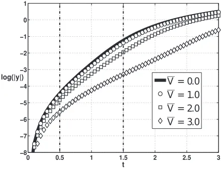
in Fig.2 which superimposes the linear stability curves at different values of ¯V (labelled) along with corresponding growth rates predicted by DNS at the respective values of ¯V (also labelled). We notice striking agreement for both perturbation wavenumbers, and observe the stabilizing effect of the electric field as ¯V is increased; the maximum growth rate decreases and the corresponding wavelength shifts to longer lengths as the band of unstable wavenumbers decreases. The least squares fit errors in estimating growth rates are less than 0.8% in all cases presented. Fig.3is used to explain the growth rate extraction procedure in more detail. The plot shows the evolution of the logarithm of the absolute value of the interface minimum|y|, say. We identify an exponential growth regime when the log-curve follows a straight line after an initial transient. The interval 0.5t1.5 identified by
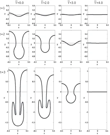
[image:8.612.194.414.534.704.2]FIG. 4. Snapshots of the interfacial position att=1 (top row),t=2 (middle row), andt=3 (bottom row), for increasing values of the applied electric potential difference ¯V=0,2,3,4. The evolution for the designated value of ¯Vis contained in each of the four columns and the field increases from left to right. Other flow parameters are as given in Fig.2.
the two dashed vertical lines, approximately defines the extent of the linear regime in this particular example. The slope of the curves for each ¯V is calculated using a least squares fit and the results are added to Fig.2as appropriate symbols. The reason that an initial adjustment is required before the solution follows the predictions of linear theory is due to the fact that only the interface is perturbed att=0, while the velocities, pressures, and electric fields are not disturbed.
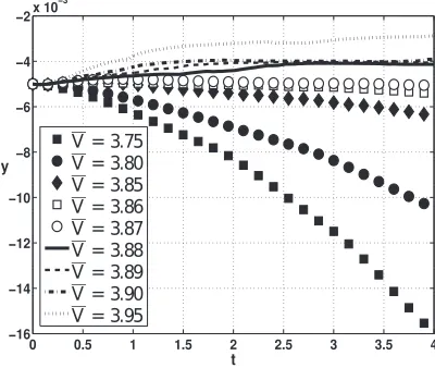
FIG. 5. Computation via DNS of the critical stabilizing voltage potential difference ¯V. The evolution of the positionyof the interface minimum is shown for a set of values of ¯Vclose to the theoretically predicted value ¯Vc≈3.867 given by linear
theory. Other parameters are as in Fig.2.
delayed. For example, looking at the profiles att=3 (last row of panels) the length of the finger in the absence of an electric field is approximately 2.8 units, it is approximately 2.1 units when ¯V =2, and it decreases further to approximately 1.1 units when ¯V =3; when ¯V =4 there is no finger due to complete stabilization. In addition, the roll-up structures att=3 become much less pronounced as ¯V increases and are hardly discernible above ¯V =3. Hence, we can conclude that the electric field can be used to control the nonlinear features of Rayleigh-Taylor instability and can in principle be selected to obtain a finger of a given length at a given time.
Next we evaluate the capabilities of the code in identifying the critical strength of the electric field above which the flow becomes linearly stable. For the same flow parameters used earlier in this section, linear stability theory predicts that disturbances with wavenumberk=2π are completely stabilized above the critical value ¯Vc=3.867. Fixing the global accuracy of the simulations to be
of order 10−3, and the initial perturbation amplitude to be 5×10⁻³ as before, we wish to verify
that the code can reproduce this value of ¯Vcwithin the computational error bounds. To achieve this
we simulate with ¯V taking values from 3.75 to 3.95, with a more refined set of values around ¯Vc.
Fig.5summarizes these numerical experiments; the curves consisting of open circles ( ¯V =3.87) and squares ( ¯V =3.86) represent the parameter regime we are trying to identify since ¯Vclies within
these two values. The plot describes the evolution of the interface minimum for sufficiently long times to enable a clear distinction between stable or unstable flows. The minimum starts at a value of 5×10⁻³att=0, and either increases to 0 or to more negative values depending on whether the flow is stable or unstable, respectively. These results show that the direct numerical solutions are highly accurate and are capable of predicting critical parameters that delineate stability and instability windows.
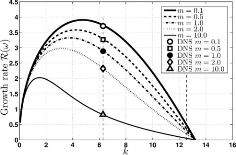
2. Effect of the viscosity ratio m
The computations in Sec.IV A 1were carried out for fluids of equal viscosities. In numerous applications viscosities differ (sometimes severely) and in what follows we consider the effect of the viscosity ratiom=μ2/μ1(upper to lower fluid values) on the electrostatic stabilization mechanism
FIG. 6. Comparison between linear theory and DNS for different viscosity ratios as labeled in the legend. The continuous curves correspond to linear theory and the symbols come from DNS. Other parameters are as in Fig.2.
The results show that an increase inmabove unity reduces the growth rate and this stabilization becomes more pronounced with increasingm. At the same time, the instability increases asmis decreased below unity since the less viscous fluid on top experiences less internal friction and flows faster under gravity. The numerically obtained results via DNS for a wavenumber 2π(q=1 in(29)), show excellent agreement with the analytically predicted values. Low viscosity fingers penetrating into more viscous fluid are more prone to develop “mushroom-shaped” roll-up structures as those seen in Fig.4, while a higher viscosity in the top fluid inhibits growth and acts as a delay mechanism for nonlinear effects—this is discussed in more detail in Sec.IV C. A noteworthy observation is that the critical wavenumber where the flow becomes stable is not affected by changes in viscosity ratio. This has been confirmed by considering the inviscid limit of the problem. We rederived the following explicit inviscid dispersion relation for our model,
ω2(k)=g˜1−r
1+r|k| −σ˜ r 1+r|k|k
2− r
1+r
(1−p)2
1+p
¯
V2k2. (30)
The first term on the right-hand side is responsible for the classical Rayleigh-Taylor instability and is driven by the density ratio between the two fluids (r=ρ1/ρ2 <1 corresponds to a heavier
fluid on top). The other two terms (surface tension and electric field) are both stabilizing and in fact produce dispersive effects. Note that an exactly analogous stabilizing effect (instead of ¯V2
one obtains ¯H2 where ¯H is the strength of the applied magnetic field) has been found in the
linear analysis of Chandrasekhar3 (Section 97, pp. 464–466), in the case of a horizontal mag-netic field applied to inviscid fluids of zero resistivity. The qualitative instability features are as found previously (see Fig. 2, for instance) with enhanced stabilization as surface tension and/or electric field effects increase. Sufficiently long waves will always be unstable but in the finite geometries computed here a complete stabilization can emerge. More specifically, for the param-eters used in Fig.6but neglecting viscous effects, relation(30)provides a critical ¯Vci =3.867708
for the inviscid limit, which is almost identical to that deduced from the viscous dispersion relation.
Having established that a sufficiently strong electric field can completely stabilize the flow, next we consider such regimes in order to evaluate the code’s accuracy and capabilities in capturing interfacial oscillations that are temporally damped (either monotonically (overdamped), or in an oscillatory manner (underdamped)).
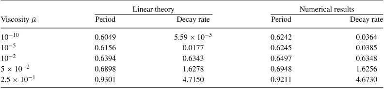
B. Linearly stable regime
When the flow is linearly stable the eigenvalueωis generally complex, i.e.ω=ωr+iωi, with
FIG. 7. Comparison between linear theory and DNS in a regime that is stable according to linear theory. Solid curve – linear theory. Open circles – DNS. The value of the viscosity ratio is ˜μ=0.01. Other parameters are ˜ρ1=1, ˜ρ2=2, ˜σ=1.5, ˜
g=9.80655, ˜1=1, ˜2=2, and ¯V=1.
the evolution of the interface at the midpointx=0, that is definingS0(t)=S(x=0,t), linear theory
predicts
S0(t)=Ai cos(|ωi|t)e−|ωr|t. (31)
For this set of numerical experiments we use ˜ρ1=1, ˜ρ2=2, ˜σ =1.5, ˜g=9.80655, ˜1 =1, ˜2=2,
¯
V =1 and ˜μvaries from 10−10(close to inviscid) to 0.25. The viscosities in the two fluids are taken
to be equal, hencem=1. The initial perturbation amplitude is now slightly higher, 5×10⁻², in
order to enable a sufficient number of resolvable damped oscillations.
An example of the dynamics ofS0(t) for dimensionless viscosity ˜μ=0.01 is shown in Fig.7.
The figure superimposes the analytical result(31)(withAi=5×10⁻²andωcalculated from the
implicit dispersion relation) with the evolution ofS0(t) predicted from DNS. Agreement is very good
and we can conclude that the code is fully capable of predicting the damped oscillatory behavior that characterizes the flow in this regime. It is worth noting that the oscillations depend crucially on the presence of the electric field - in its absence the flow is Rayleigh-Taylor unstable for these parameters. Physically, then, the electric field causes a dispersive stabilization and the non-zero viscosity provides the damping seen in the results. We also note that plots similar to Fig.7were used to accurately extract both the decay-rate as well as the period of the damped oscillations for a wide range of dimensionless viscosities ˜μ. This is done by considering local extrema in the oscillation, and locally fitting a polynomial to the coordinates in the vicinity of consecutive peaks. The results are collected in TableI; the second and third columns provide the analytical linear stability results while the corresponding period and decay rates computed by DNS are given in the last two columns, respectively. Agreement is very good with the exception of the two smallest viscosity values ˜μ=10−10,10−5 that were selected to push the code into an inviscid regime. In
TABLE I. Study of the oscillatory motion of the interface in linearly stable regimes for different viscosities.
Linear theory Numerical results
Viscosity ˜μ Period Decay rate Period Decay rate
10−10 0.6049 5.59×10⁻⁵ 0.6242 0.0364
10−5 0.6156 0.0177 0.6245 0.0385
10−2 0.6394 0.6343 0.6497 0.6348
5×10⁻² 0.6898 1.6278 0.6948 1.6256
[image:12.612.107.503.634.726.2]these two cases the period is overestimated by the simulations and the decay rate is higher than predicted. It is also worth noting that the DNS predictions for these two viscosities are very similar even though the viscosity values are different by five orders of magnitude. This is in part due to the numerical viscosity imposed by default in GERRIS for stability and to limit artifacts. Discretization schemes typically introduce small amounts of numerical viscosity, and even though the code has strong optimizations in this direction, our results indicate that there is a clear limit on how small the viscosity can be.
At values of the viscosity of 10−2or larger, however, there is very good agreement and the code
is very robust. For example, for the largest value ˜μ=2.5×10⁻¹the decay rate is quite fast and the
DNS results capture this and the period of oscillation with considerable accuracy (the errors are less than 1%). In all these simulations the final time was taken to bet=3 which proved proved effective in capturing decay rates and periods of oscillation but is also large enough to reach trivial steady states in the more viscous cases.
The main aim of the results described thus far has been the validation of the linear stability theory with direct numerical simulations. We presented a comprehensive set of results in both linearly stable and unstable regimes, which establish solid agreement between theory and DNS using GERRIS. Armed with the positive outcomes of these stringent tests we continue our investigation with numerical experiments into the fully nonlinear regime.
C. Fully nonlinear stage
The results of Fig.4presented the broad qualitative aspects of the nonlinear stages of electrified Rayleigh-Taylor instability in viscous stratified fluids. In the non-electrified case such features (penetrating fingers that roll up) have been observed in experiments and simulations by other authors; in what follows we quantify analogous nonlinear structures with particular emphasis placed on the electric field effects. One important feature is the position (length) of penetrating viscous fingers into lighter fluid and the speed of the finger tip. To this end we define the finger tip position by y(t)=S(0,t), track its evolution and estimate the downward tip speed|dy/dt|by applying backward differences in time. We begin by presenting the effect of the applied electric potential difference ¯Von tip dynamics, and conclude by showing a simple active control procedure using the electric field that results in setting the unstable interface into externally forced sustained time-periodic oscillations.
1. Electric field effects on finger dynamics
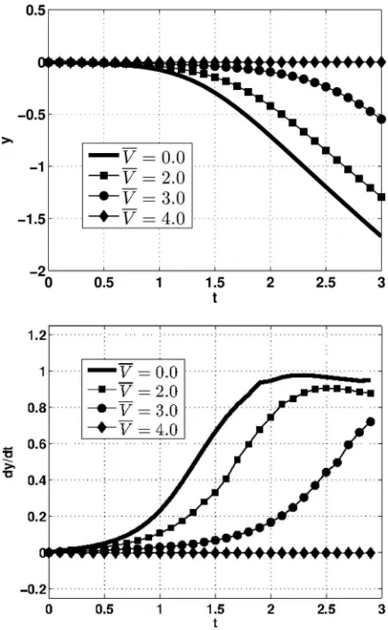
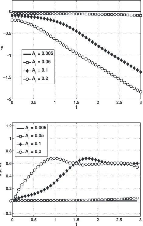
FIG. 8. Evolution of the interface minimumy(t)=S(0,t) (top panel) and its speed (bottom panel), as the electric potential difference ¯Vincreases. Other parameters are as in Fig.2.
The results presented so far strongly indicate that a sufficiently large electric field can completely stabilize the flow. In the next set of computations we investigate this mechanism in more detail as a function of the initial perturbation of the interface. A particular question of interest is whether for a given electric potential difference ¯V, there exists a threshold initial amplitude above which the Rayleigh-Taylor instability will dominate over the electrostatic Maxwell stresses (for fixed surface tension forces) and the usual fingers will form. To best evaluate the role of initial conditions we select ¯V =4 so that the flow is linearly stable in this regime. Computations are carried out for initial amplitudes ranging from relatively small valuesAi =0.005, 0.05 to relatively large values
Ai=0.1, 0.2 (note that the caseAi=0.005 has already been shown to predict full stabilization).
The evolution of the tip positiony(t) and the corresponding tip speed|dy/dt|are given in Fig. 9
in the top and bottom panels, respectively. The results show that the electric field in this case is not capable of arresting the growth of initial disturbances beyond a threshold value that increases with ¯V. For ¯V =4 an initial amplitudeAi=0.05 appears to be just above such a threshold since
FIG. 9. Role of initial perturbation amplitudesAi(as labeled) for the case ¯V=4 that is predicted to be stable by linear theory
(other parameters are as in Fig.2). The top panel shows the evolution of the interface minimumyand the bottom panel the corresponding speed of this tip. Amplitudes larger than 0.05 overcome the electric field stabilization mechanism and lead to a nonlinear evolution.
particularly visible for the largest initial amplitude used, Ai =0.2 after approximately 2.75 time
units).
The numerical results described in this section have shown that the code is fully capable of capturing the physics of the problem and is in complete quantitative agreement with linear stability theory. The code provides us with a computational tool to investigate the fully nonlinear regime and in particular to utilize of the electric field to produce desirable flow features such as sustained large amplitude interfacial oscillations that can be useful in mixing. Such phenomena arising from prescribed electric field variations are described next.
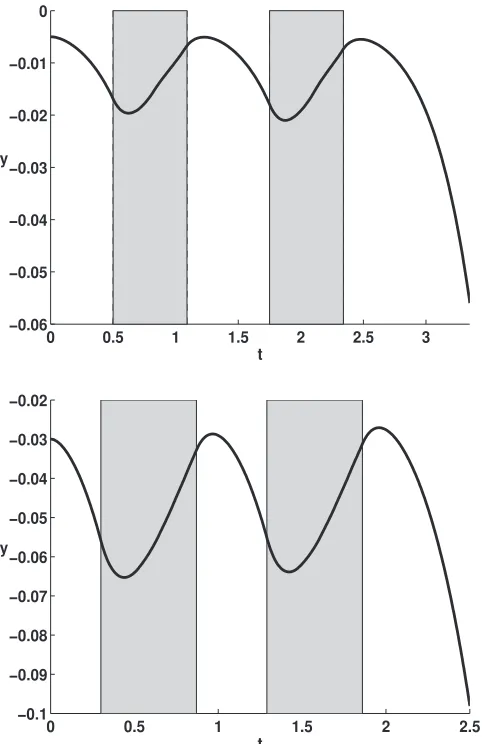
D. Inducing time-periodic interfacial oscillations using the electric field
Our objective here is to utilize the electrostatic stabilization mechanisms described above to construct a way of producing ordered time-periodic fluctuations of the interface. The ultimate aim, from a practical perspective, is to identify active control protocols that induce time dependent flows in small scale devices without the need for moving parts, and to use such flows for mixing in small-scale geometries.
FIG. 10. Inducing sustained interfacial oscillations in a regime that is Rayleigh-Taylor unstable in the absence of an electric field ( ˜ρ1=1, ˜ρ2=5, ˜μ=0.25,m=1, ˜g=9.80655, ˜σ=0.2, ˜1=1, ˜2=2). Results are shown for an initial perturbation amplitudeAi=0.005 (top panel) and a much larger amplitudeAi=0.03 (bottom panel). The electric field is switched on
with a difference in voltage potential of ¯V=5 during the gray intervals and off during the white ones. An arbitrary number of oscillations can be induced by successively repeating the on-off protocol.
As described earlier, if ¯V =0 the flow is unstable and a downward penetrating finger forms, whereas with ¯V =4 the flow can be completely stabilized (see the results of Fig.4, for example). This opens the way for generating sustained oscillations as follows: (i) Start with no field and allow the flow to become unstable; (ii) switch on the field to stabilize the flow and cause the interface to move upwards; (iii) switch off the field again to generate an instability and finger formation; (iv) repeat the process to obtain a time-periodic oscillation. Clearly the parameters must be tuned for a given initial perturbation amplitude, and we emphasize that the initial amplitudes cannot be too large (see the results of Sec.IV C 1and particularly Fig.9). Although the generation of time-periodic oscillations introduces a time-dependent electric field, the quasi-static approximation is still valid (see AppendixB) and the analytical and numerical treatments considered in Secs.IV A–IV Chold.
In the computations presented here we demonstrate the resulting oscillatory flows for relatively small (Ai=0.005) and relatively large (Ai=0.03) amplitudes; in both cases we fix ¯V =5 which is
sufficiently strong to stabilize the flow. The results are depicted in Fig.10that shows the evolution of y(t)=S(0,t); the top panel corresponds to the weaker initial perturbation Ai=0.005 and the
bottom panel toAi=0.03. During the gray-shaded intervals the field is on, and it is off elsewhere. In
Ai=0.03 case), and they are alternated by field-off intervals so as to attain a time-periodic oscillation
of the whole interface similar to a standing wave (not shown for brevity). Intuitively, the field is turned on once the finger forms and is developing into the nonlinear regime of finger formation and penetration, kept on until the flow is stabilized, and then switched off again to allow the finger to form once more. Repeating the process produced the depicted oscillations in time. The adopted protocol is quite simple and has been selected for illustrative purposes rather than with the goal of optimization of certain quantities. Such lines of investigation are currently under way and beyond the scope of the present work.
V. DISCUSSION AND CONCLUSION
We have investigated theoretically, through linear stability theory and direct numerical simula-tions, the effect of electric fields on stratified viscous flows that are susceptible to the Rayleigh-Taylor instability. The simulations have been based on volume-of-fluid methods through the GERRIS29 plat-form, and the main focus has been on the stabilizing effects of a uniform electric field imposed in the horizontal direction (parallel to the undisturbed interface). Computational studies were performed for a range of system parameters that include both stably and unstably stratified regimes. The volume-of-fluid based code, with its adaptive mesh refinement and specialized algorithms for the problem in question, was found to produce accurate results in reasonable CPU times and has been validated to be in excellent agreement with the analytical predictions of linear theory (an implicit dispersion relation has been derived and used—see Sec.III).
Stringent quantitative validation studies of DNS with linear theory have been carried out with growth rates estimated through DNS starting from small initial perturbations. This has been done both in the unstable regime where primary exponential growth rates are computed and compared (see Figs.2and6for a range of applied voltage parameters ¯V and viscosity ratiosm, respectively), and in the stable regime where oscillation frequencies and damping rates are estimated from the simulations and compared with the analytical results (see Fig. 7 and Table I). In both cases agreement is compelling thus furnishing us with a suitable computational tool to explore the fully nonlinear regime. We have demonstrated the ability of the electric field to affect nonlinear features of the Rayleigh-Taylor instability (see Fig.4). As the magnitude of the applied electric potential increases, the length of the finger at a given time, decreases, and more interestingly the instability can be completely suppressed for fields above critical strength. The critical field strengths when complete stabilization is achievable, have been found to be in very close agreement with the critical values predicted by linear theory (see Sec.IV A 1and Fig.5). Our simulations also indicate that for a fixed electric field strength, the Rayleigh-Taylor instability cannot be suppressed if the initial perturbation amplitude is large enough – see for example, Fig.9where a field characterized by voltage potential difference
¯
V =4 is not capable of stabilizing disturbances of amplitudes larger than 0.05. As ¯V increases further, flows starting from larger initial amplitudes can be completely stabilized, but we have limited the computations presented here to physically reasonable values of ¯V, as discussed below also.
Having illustrated the stabilization phenomena (both in the linear and nonlinear regime), we showed how sustained interfacial oscillations can be produced by imposing a time-periodic electric field. This was achieved by simply switching the field on and off in succession, so that its action is used to stabilize the flow during the finger formation stage, after which it is switched off to enable the instability to take place and the finger to form once more, with the process repeating at will. The resulting flow produces a time-periodic oscillation of the interface (and consequently spatio-temporal dynamics in the bulk) – typical results of the ensuing periodic motion are shown in Fig.10– and we suggest that such protocols could be useful in mixing applications in small-scale geometries.
in experiments,30,31it is feasible to carry out simulations using our computational tools to determine necessary stabilizing field strengths.
A suitable example is that of water for the top fluid 1, and olive oil for the lower fluid 2— see the schematic in Fig.1. The physical properties of these fluids can be summarized as fol-lows. Water at 20◦C has density ρ2 =998.207 kg/m3, viscosity μ2 = 8.95 × 10⁻⁴ Pa s, and
electrical permittivity2 =80.40, where0=8.85×10⁻¹² m−3kg−1s4A is the permittivity of
free space. The equivalent properties for olive oil are ρ1 =918 kg/m3, μ1 = 0.081 Pa s, and
1 =3.10. The surface tension between olive oil and water is 0.02 kg s−2. We use a channel of
width 0.035 m under the action of a gravitational acceleration of 9.80655 m s−2. From the linear
theory of Sec.III we deduce that without the action of an electric field the system is prone to instability. In order to completely stabilize the system we derive the critical strength of the electric field to be Ec ≈2.032×10⁴ V/m, which is well within the range of experimentally attainable
values. This result holds for an initial perturbation of wavenumberk=2π, which corresponds to the largest (and most dangerous) wavelength that can be imposed in our numerical environment. Note also that the predicted field valueEcis significantly below the dielectric breakdown limits which
are approximately 1.35×10⁷V/m for water39and 1.755×10⁷V/m for vegetable oils,40respectively. The two fluids used in this example are commonly found in applications and there are numerous other fluids of industrial significance, as for example, systems containing water and 1−octanol, or water and carbon tetrachloride.
ACKNOWLEDGMENTS
The work of D.T.P. and P.G.P. was in part supported by the National Science Foundation (Grant No. DMS-0707339). The work of D.T.P. was also supported by EPSRC grant EP/K041134/1; R.C. acknowledges a Roth Doctoral Fellowship from the Department of Mathematics, Imperial College London.
APPENDIX A: DISPERSION RELATION DETAILS
In Sec.III, we described the solution procedure to obtain an implicit dispersion relation for the growth rateω(k) as a function of wavenumber and the physical parameters. This hinges on finding non-trivial solutions toMX=0, whereMrepresents the coefficient matrix andXis the vector of unknownsX=[AS C˘ 1C2 P1 P2]T. For completeness we provide the non-zero entriesMijof the 6
×6 matrixMas they arise from the boundary conditions(11)–(14).
The first row is taken to be the contribution from the continuity of the normal component of the displacement field(15):M11= |k|(p+1),M12=i k(p−1) ¯V.
The kinematic condition for the first fluid given by(11)provides the second row:M22 =ω,
M23=
i k√μ˜
k2μ˜+ω,M25 =
k2
|k|(k2μ˜+ω− |k|2μ˜).
Manipulating the continuity of tangential stress balance (13) results in the entries
of the third row: M33 =
k2μ˜ +ω
√
˜
μ +
k2√μ˜
k2μ˜+ω, M34=m
k2m˜μr+ω
√
mμ˜r +m
k2√mμ˜r
k2mμ˜r+ω,
M35= −
i k|k|2+i k3
|k|(k2μ˜ +ω− |k|2μ˜),M36 = −m
i k|k|2r+i k3r |k|(k2mμ˜r+ω− |k|2mμ˜r).
Continuity of normal stresses, with an explicit expression given as (12), yields: M41= −i kV¯(1−p), M42= gr˜(r−1)+k
2σ˜, M
43= −2i kμ˜, M44=2i kmμ˜, M45= −1
− 2 ˜μk2
k2μ˜+ω− |k|2μ˜,M46=1+
2mμ˜k2r
k2mμ˜r+ω− |k|2mμ˜r.
The two velocity field components produce the final two rows of entries in matrix M. The
continuity description found in (14) gives M53 = 1, M54 = −1, M55 = −
i k
k2μ˜ +ω− |k|2μ˜,
M56=
i kr
the vertical velocity component vproduces entriesM63= −
i k√μ˜
k2μ˜ +ω,M64= −
i k√mμ˜r
k2mμ˜r+ω,
M65= −
k2
|k|(k2μ˜ +ω− |k|2μ˜),M66 = −
k2r
|k|(k2mμ˜r+ω− |k|2mμ˜r).
The desired transcendental eigenrelation is found by setting det(M)=0.
APPENDIX B: JUSTIFICATION OF THE APPLICABILITY OF THE ELECTROSTATIC LIMIT
We consider a simple scaling argument to justify why the existence of a magnetic field can be ignored at leading order in our analysis. Starting from the magnetic induction equation
∇ ×H=J+∂E
∂t , (B1)
whereHis the magnetic field andJis the current, we use the following approach. By construction, the electric field is scaled byE0∼V¯∗/Land we writeH=H0Hand continue in simplified notation
(dropping the primes for convenience). We are particularly interested in the effect of frequency with which the electric field is switched on and off in the example at the end of SubsectionIV D. Using the induction equation(B1)yields
H0∼0E0L. (B2)
Considering the approximations0∼10−11F m−1,L ∼10−2m, and typical electric field strength
E0∼104V m−1, which are standard values within the context of our desktop experiments, gives
H0∼10−9T s, (B3)
measured in an appropriate timescale 1/, where T denotes teslas and s seconds. We argue that within the current framework values of that would yield a sufficiently high value of H0 are never reached. The time scale leading to the dimensionless momentum equations (8) is
(L/g)1/2 (the velocity scale is proportional to√g L). Considering centimeter-sized geometries, so
L ∼O(10−2), our dimensional times are approximately 101–102 s. Note that a cycle in the on-off
protocol described in the subsection of interest develops over one dimensionless time unit, therefore
∼10−2–10−1 Hz. This bringsH
0 down to less than 10−10 T and hence the contribution of the
magnetic field is negligible. We point out that even if we wish to model a system with a much higher frequency of the on-off protocol, in the kilohertz range or even more, the induced magnetic field would still be of very small scale and would play an inconsequential role in this study. The result follows from previous explorations of this limit.41
1Lord Rayleigh, “Investigation of the character of the equilibrium of an incompressible heavy fluid of variable density,”
Proc. London Math. Soc.14, 170 (1883).
2G. I. Taylor, “The instability of liquid surfaces when accelerated in a direction perpendicular to their planes. I,”Proc. R.
Soc. London, Ser. A201, 192 (1950).
3S. Chandrasekhar,Hydrodynamic and Hydromagnetic Stability(Oxford University Press, Oxford, 1961), pp. 428–453. 4A. J. Babchin, A. L. Frenkel, B. G. Levich, and G. I. Sivashinsky, “Non-linear saturation of Rayleigh-Taylor instability in
thin films,”Phys. Fluids26, 3159 (1983).
5D. Halpern and A. L. Frenkel, “Saturated Rayleigh-Taylor instability of an oscillating Couette film flow,”J. Fluid Mech.
446, 67 (2001).
6D. T. Papageorgiou, C. Maldarelli, and D. S. Rumschitzki, “Nonlinear interfacial stability of core-annular flows,”Phys.
Fluids A2, 340 (1990).
7B. J. Lowry and P. H. Steen, “Stability of slender liquid bridges subjected to axial flows,”J. Fluid Mech.330, 189 (1997). 8O. Haimovich and A. Oron, “Nonlinear dynamics of a thin liquid film on an axially oscillating cylindrical surface,”Phys.
Fluids22, 032101 (2010).
9D. E. Weidner, L. W. Schwartz, and M. H. Eres, “Simulation of coating layer evolution and drop formation on horizontal
cylinders,”J. Colloid Interface Sci.187, 243 (1997).
10Z. Huang, A. De Louca, T. J. Atherton, M. Bird, and C. Rosenblatt, “Rayleigh-Taylor instability experiments with precise
and arbitrary control of the initial interface shape,”Phys. Rev. Lett.99, 204502 (2007).
11J. R. Melcher, “Electrohydrodynamic and magnetohydrodynamic surface waves and instability,”Phys. Fluids4, 1348 (1961).
13G. I. Taylor and A. D. McEwan, “The stability of a horizontal fluid interface in a vertical electric field,”J. Fluid Mech.22,
1 (1965).
14E. Schaffer, T. Thurn-Albrecht, T. P. Russell, and U. Steiner, “Electrically induced structure formation and pattern transfer,”
Nature403, 874 (2000).
15N. Wu and W. B. Russel, “Micro- and nano-patterns created via electrohydrodynamic instabilities,”Nano Today4, 180
(2009).
16J. R. Melcher and E. P. Warren, “Continuum feedback control of a Rayleigh-Taylor type instability,”Phys. Fluids9, 2085 (1966).
17B. S. Tilley, P. G. Petropoulos, and D. T. Papageorgiou, “Dynamics and rupture of planar electried liquid sheets,”Phys.
Fluids13, 3547 (2001).
18K. Savettaseranee, D. T. Papageorgiou, P. G. Petropoulos, and B. S. Tilley, “The effect of electric fields on the rupture of
thin viscous films by van der Waals forces,”Phys. Fluids15, 641 (2003).
19D. T. Papageorgiou and J.-M. Vanden-Broeck, “Large-amplitude capilarry waves in electrified fluid sheets,”J. Fluid Mech.
508, 71 (2004).
20S. Grandison, D. T. Papageorgiou, and P. G. Petropoulos, “Interfacial capillary waves in the presence of electric fields,”
Eur. J. Mech. B: Fluids26, 404 (2007).
21R. J. Raco, “Electrically supported column of liquid,”Science160, 311 (1968). 22G. I. Taylor, “Electrically driven jets,”Proc. R. Soc. London, Ser. A313, 453 (1969).
23S. Sankaran and D. A. Saville, “Experiments on the stability of a liquid bridge in an axial electric field,”Phys. Fluids A5, 1081 (1993).
24A. Ramos, H. Gonzalez, and A. Castellanos, “Experiments on dielectric liquid bridges subjected to axial electric fields,”
Phys. Fluids6, 3206 (1994).
25C. S. Burcham and D. A. Saville, “The electrohydrodynamic stability of a liquid bridge: microgravity experiments on a bridge suspended in a dielectric gas,”J. Fluid Mech.405, 37 (2000).
26L. L. Barannyk, D. T. Papageorgiou, and P. G. Petropoulos, “Supression of Rayleigh-Taylor instability using electric fields,”
Math. Comput. Simul.82, 1008 (2012).
27N. T. Eldabe, “Effect of a tangential electric field on Rayleigh-Taylor instability,”J. Phys. Soc. Jpn.58, 115 (1989). 28A. Joshi, M. C. Radhakrishna, and N. Rudraiah, “Rayleigh-Taylor instability in dielectric fluids,”Phys. Fluids22, 064102
(2010).
29S. Popinet, “Gerris: A tree-based adaptive solver for the incompressible Euler equations in complex geometries,”J. Comput.
Phys.190, 572 (2003).
30A. Bagu´e, D. Fuster, S. Popinet, R. Scardovelli, and S. Zaleski, “Instability growth rate of two-phase mixing layers from a
linear eigenvalue problem and an initial-value problem,”Phys. Fluids22, 092104 (2010).
31D. Fuster, A. Bagu´e, T. Boeck, L. Le Moyne, A. Leboissetier, S. Popinet, P. Ray, R. Scardovelli, and S. Zaleski, “Simulation of primary atomization with an octree adaptive mesh refinement and VOF method,”Int. J. Multiphase Flow35, 550 (2009). 32J. M. L´opez-Herrera, S. Popinet, and M. A. Herrada, “A charge-conservative approach for simulating electrohydrodynamic
two-phase flows using volume-of-fluid,”J. Comput. Phys.230, 1939 (2011).
33H. H. Woodson and J. R. Melcher,Electromechanical Dynamics, Part III: Elastic and Fluid Media(Wiley, New York, 1968), pp. 783–789.
34D. A. Saville, “Electrohydrodyanmics: The Taylor-Melcher leaky dielectric model,”Annu. Rev. Fluid Mech.29, 27 (1997). 35C. S. Burcham and D. A. Saville, “Electrohydrodynamic stability: Taylor-Melcher theory for a liquid bridge suspended in
a dielectric gas,”J. Fluid Mech.452, 163 (2002).
36S. Popinet, “An accurate adaptive solver for surface-tension-driven interfacial flows,”J. Comput. Phys.228, 5838 (2009). 37S. Mahlmann and D. T. Papageorgiou, “Numerical study of electric field effects on the deformation of liquid drops in
simple shear flow at arbitrary Reynolds number,”J. Fluid Mech.626, 367 (2009). 38J. D. Jackson,Classical Electrodynamics(Wiley, New York, 1967), pp. 116–119.
39W. A. Stygar, M. E. Savage, T. C. Wagoner, L. F. Bennett, J. P. Corley, G. L. Donovan, D. L. Fehl, H. C. Ives, K. R.
LeChien, G. T. Leifeste, F. W. Long, R. G. McKee, J. A. Mills, J. K. Moore, J. J. Ramirez, B. S. Stoltzfus, K. W. Struve, and J. R. Woodworth, “Dielectric-breakdown tests of water at 6 MV,”Phys. Rev. ST Accel. Beams12, 010402 (2009). 40M. Marci and I. Kolcunova, “Electric breakdown strength measurement in liquid dielectrics,” inProceedings of the 9th
International Conference on Environment and Electrical Engineering (EEEIC), Prague, Czech Republic, 16–19 May 2010
(IEEE, 2010), p. 427.