Point process modelling of coordinate based meta analysis neuroimaging data

(1)

warwick.ac.uk/lib-publications

A Thesis Submitted for the Degree of PhD at the University of Warwick

Permanent WRAP URL:

http://wrap.warwick.ac.uk/87635

Copyright and reuse:

This thesis is made available online and is protected by original copyright.

Please scroll down to view the document itself.

Please refer to the repository record for this item for information to help you to cite it.

Our policy information is available from the repository home page.

(2)

Point process modelling of

coordinate-based meta-analysis

neuroimaging data

by

Pantelis Samartsidis

Thesis

Submitted to the University of Warwick

for the degree of

Doctor of Philosophy

Department of Statistics

(3)

Sta kor–tsia (Mar–a, Tatiàna, Eir†nh)

-... Qàrhka pàra pol‘ k‘rie BlammËne! -Mh me lËte blammËno.

-Afo‘ BlammËno sac lËne,pwc na sac p∏; -DÏktwr.

-Aaaa,dÏktwr. Kaj†ste dÏktwr! ...

(4)

List of Tables

3.1 Extract from a CBMA dataset of emotion studies . . . 12

4.1 LGCP simulation study 1 results: posterior summaries . . . 40

5.1 Group fMRI simulation study: setup for study centers . . . 66

6.1 Estimated posterior prevalence of zero-count studies for subsamples

A-E . . . 91

A.1 Meta-analysis of emotion and executive control studies: ROI analysis for emotions . . . 113 A.2 Meta-analysis of emotion and executive control studies: ROI analysis

for executive control . . . 116

C.1 Zero-truncated Negative Binomial simulation study: bias of ˆp0 . . . 153

(8)

List of Figures

2.1 An average brain in MNI space . . . 5

3.1 Graphical representation of the BHICP . . . 19

3.2 ALE simulation study: power against the proportion of valid studies 23

3.3 ALE simulation study: power against the total number of valid studies 24

3.4 Results of the meta-analysis of 164 emotion studies using ALE, MKDA,

SDM and the BHICP . . . 27

4.1 LGCP simulation study 1: type 1 true and estimated latent Gaussian

fields in slicesz= 22 andz= 4 . . . 41

4.2 LGCP simulation study 1: type 2 true and estimated latent Gaussian

fields in slicesz= 22 andz= 4 . . . 42

4.3 LGCP simulation study 2: estimated latent Gaussian fields and mean

standardised posterior di↵erence in slicez = 24 . . . 45

4.4 LGCP simulation study 2: estimated latent Gaussian fields and mean

standardised posterior di↵erence in slicez = 16 . . . 46

4.5 Graphical representation of the meta-analysis dataset consisting of

855 emotion and 338 executive control studies . . . 47

4.6 Meta-analysis of emotion and executive control studies: median

pos-terior intensity for emotions . . . 49

4.7 Meta-analysis of emotion and executive control studies: median

pos-terior intensity for executive control . . . 50

4.8 Meta-analysis of emotion and executive control studies: mean

stan-dardised posterior di↵erence of the two types . . . 51

4.9 Meta-analysis of emotion and executive control studies: estimated

posterior probabilities of observing at least one focus for several ROIs 53

5.1 Realisation of the group fMRI model for 3 participants . . . 62

(9)

5.3 Group fMRI simulation study: participant 8 results . . . 69

5.4 Group fMRI simulation study: traceplots forn x+₁ ,n x₁ ,n x+₈ ,

n x8 ,n(z+) andn(z ) . . . 71

5.5 Group fMRI simulation study: voxel-wise posterior probability of

observing a study center . . . 72

5.6 Group fMRI simulation study: component sensitivity tom . . . 75

5.7 Group fMRI simulation study: center sensitivity tom . . . 76

5.8 Group fMRI simulation study: true positive rate sensitivity tom . . 77

5.9 Group fMRI study on faces task: center sensitivity analysis . . . 81

5.10 Group fMRI study on faces task: voxel-wise posterior probability of

observing a study center . . . 82

5.11 Group fMRI study on faces task: participant 1 results . . . 83

6.1 Empirical distribution of the total number of foci per experiment in

the BrainMap database . . . 88

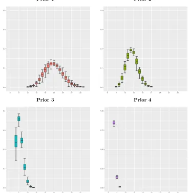
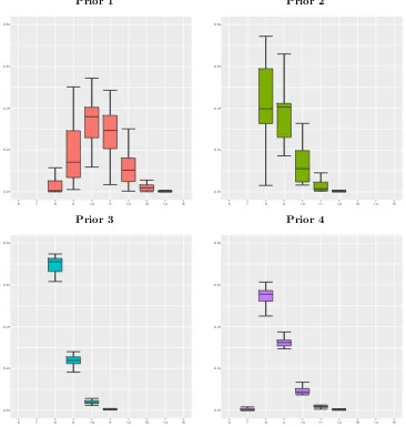
6.2 Zero-truncated Poisson and Negative Binomial fit for subsample A . 92

6.3 Estimated posterior prevalence of zero-count studies as function of

study year and sample size for subsample A . . . 92

6.4 Estimated prevalence of zero-count studies as a function of study

context for subsample A . . . 93

6.5 Estimated posterior probabilities of observing at least one activation

the right and left amygdala, before and after the inclusion of

zero-count studies . . . 95

A.1 LGCP simulation study 1: traceplots for k and ⇢k . . . 104

A.2 LGCP simulation study 1: traceplots forµk and k . . . 105

A.3 Meta-analysis of emotion and executive control studies: traceplots

and ACFs for k . . . 106

and ACFs for⇢k . . . 107

and ACFs forµk . . . 108

and ACFs forR_B k(⇠)d⇠ . . . 109

and ACFs for k

v1 . . . 110

(10)

A.9 Meta-analysis of emotion and executive control studies: posterior

pre-dictive check on first order properties . . . 120

A.10 Meta-analysis of emotion and executive control studies: posterior pre-dictive check on second order properties . . . 121

B.1 Group fMRI study on faces task: traceplots for n x+_i and n x_i , i= 1, . . . ,3 . . . 136

B.2 Group fMRI study on faces task: traceplots for n x+_i and n x_i , i= 4, . . . ,6 . . . 137

B.3 Group fMRI study on faces task: traceplots for n(z+), n(z ), s20, m0, s2 +, m0, and s2 . . . 138

B.4 Group fMRI study on faces task: traceplots forµ+_, 2 m+, µ and _m2 139 B.5 Group fMRI study on faces task: posterior voxel-wise probability of observing an increase center with a di↵erent m . . . 140

B.6 Group fMRI study on faces task: posterior voxel-wise probability of observing an increase center with a di↵erent ⌘. . . 141

B.7 Group fMRI study on faces task: total number of participants with missing data per voxel . . . 142

B.8 Group fMRI study on faces task: participant 2 results . . . 143

C.1 Zero-truncated Poisson and Negative Binomial fit for subsamples B-E 149 C.2 Estimated posterior prevalence of zero-count studies as a function of study year and sample size for subsamples B-E . . . 150

C.3 Estimated posterior prevalence of zero-count studies as a function of study context for subsamples B-E . . . 151

(11)

Acknowledgments

First and foremost, I would like to express my deep gratitude towards my family for

their unconditional love, endless support and constant encouragement during these

past four years. Without them I wouldn’t have made it this far.

I would like to thank my supervisor Thomas Nichols for his tremendous

knowledge, guidance, motivation and patience. Our meetings have helped me

im-prove not only as a statistician, but as a person as well. I also wish to thank

Timothy Johnson for his valuable inputs on my work and the numerous interesting

discussions about statistics. Special thanks are due to Athanassios Yannacopoulos,

Vassilis Vasdekis, Petros Dellaportas and Takis Besbeas for their wonderful lectures,

their help during my undergraduate studies and for encouraging me to continue for

a PhD.

I am grateful to my flatmates Panayiota, Apostolis and Thodoris as well as

our neighbours Giorgos, Kyriaki and Loukia for all the fun, understanding, patience

and help that they have generously given. They are like a family to me. Many

thanks to my friends Habib, Simone, Giacomo, Silvia, Ioanna, Stratos, Angelos and

Fiona for all the helpful discussions regarding our research and the great times that

we shared together. Special thanks go to Helen and Murray for proofreading my

thesis.

I would like to thank all members of the Department of Statistics for creating

such a friendly and stimulating environment during my studies here at Warwick.

(12)

Declarations

This thesis is submitted to the University of Warwick in support of my application

for the degree of Doctor of Philosophy. It has been composed by myself except where

stated and has not been submitted in any previous application for any degree.

• The data for Chapter 4 were provided by Tor Wager and Lisa Feldman Barrett

• The data for Chapter 6 were obtained from the BrainMap database with help

from Angela Laird and Peter Fox

• The works in Chapters 3 and 4 are completed and will be submitted for

(13)

Abstract

(14)

Chapter 1

Introduction

Functional magnetic resonance imaging (fMRI) is a non-invasive, non-radioactive imaging technique that allows us to measure a person’s brain activity while they perform a series of tasks. fMRI is based on a fundamental link between brain activity and blood flow: when there is a rise in neuronal activity in a region of the

brain, there is also a local increase of blood flow in that region [Ogawaet al., 1990].

This so-called haemodynamic response, which arises to meet the high demands for oxygen in the area, actually leads to a surplus of local blood oxygen whose magnetic

susceptibility can then be detected by an MRI device [Kwonget al., 1992]. Hence,

one can easily establish a link between a stimulus and some brain region, just by studying the strength of the observed fMRI signal over time and throughout the brain: if a certain behaviour consistently induces a change in the fMRI signal in a certain brain region, then there is evidence that this region plays some role in the processing of the task.

This tool has motivated researchers to investigate the e↵ect of several in-teresting tasks and thus led to an explosive growth in the use of fMRI as well as significant developments in our understanding of the human brain function [Raichle, 2003]. Some examples include the di↵erences in brain function between maternal and romantic love [Bartels and Zeki, 2004], the e↵ect of alcohol while performing simulated driving [Calhoun and Pearlson, 2012] or the e↵ect of doing nothing at

all [Coleet al., 2010]. The availability of MRI scanners, inexpensive computational

resources and accessible analysis software has made fMRI an ubiquitous tool in psy-chology, neurology and psychiatry, in addition to new areas like neuromarketing

[Zurawicki, 2010] and neuroeconomics [Glimcheret al., 2008].

(15)

studies [Carp, 2012]. For example, in a recent review of emotions Lindquist et al.

[2012] found a median sample size of 11. Consequently, individual studies su↵er from

low power and hence low reproducibility [Buttonet al., 2013], and it is unsurprising

that the validity of fMRI is being challenged in both the scientific [Vulet al., 2009]

and popular [Shermer, 2008] literature (see Farah [2014] for an even-handed review). Meta-analysis, the statistical process of combining the results of indepen-dently conducted studies to increase power and obtain findings that are more likely to generalise [Hedges and Olkin, 1985], provides a natural way to address the limi-tations of single experiments (which we explain in detail in the following chapter). Meta-analysis of functional neuroimaging data is indeed an active field of research

[Wager et al., 2009; Yarkoni et al., 2010], whose growth is facilitated by the

con-stantly increasing body of literature in fMRI but also the numerous challenges that arise due the high dimensionality of single experiment data. The main challenge lies in that instead of reporting the full outcome on an fMRI experiment, that is the 3D volumes of test statistics, authors generally only report the spatial coordinates of

local maxima in significant regions of these images [Salimi-Khorshidi et al., 2009].

As a result, the standard tools that are used in meta-analyses [Hedges and Olkin,

1985; Spiegelhalter et al., 2004; Hartung et al., 2008, among others] are no longer

applicable and hence new tools need to be developed.

The objectives of this dissertation is to address the following still open prob-lems:

• Review existing approaches for fMRI meta-analysis using spatial coordinates,

explain the merits and disadvantages of these methods and identify the still open questions in the field.

• Develop a framework that enables meta-regression, the use of study

charac-teristics as covariates in fMRI meta-analysis. Such a framework can be used in order to understand the impact that these covariates have in the outcome of a study and hence explain possible di↵erences in reported results.

• Build a model for single fMRI studies that can make use of existing

meta-analysis results as prior information. This is particularly useful for studies with few participants that are underpowered and so need the input from previous studies to be able to detect subtle e↵ects.

• Estimate the file drawer quantity, the total number of studies that are missing

(16)

wrong estimates of the underlying e↵ect and thus undermine the usefulness of meta-analysis.

The thesis is organised as follows. In Chapter 2 we review some background which is used in subsequent chapters. In the first part we sketch the typical fMRI experiment so the reader becomes familiar with the particularities of the data in hand. The second part provides some theory on spatial point processes, i.e. random

sets of points in the d-dimensional Euclidian space, upon which our methods are

built. In Chapter 3 we perform a literature review of coordinate-based meta-analysis methods. The existing tools are evaluated through simulation studies and real data analysis, followed by a discussion that emphasises on strengths and weaknesses of every approach.

Chapters 4 and 5 form the main body of the text. In the former, we develop a

novel fMRI meta-analysis model based on log-Gaussian Cox processes [Mølleret al.,

1998]. The model can provide useful inferences regarding meta-analysis data and improves upon existing methods in the sense that it can account for study charac-teristics in the analysis. In the latter, Chapter 5, we present a 3 level hierarchical

model for single fMRI studies. Our method, built upon the work of Xuet al.[2009],

can be viewed as an alternative to existing approaches with the extra advantage that it addresses the problem of using meta-analysis data as prior information in new fMRI studies. In both cases, we pay special attention to the computational tools that are used to enable inferences which are carried out under the Bayesian paradigm.

(17)

Chapter 2

Background

2.1 Neuroimaging background

What follows is a very brief review of fMRI and the practical steps involved in a fMRI study. For a more detailed introduction, see Lindquist [2008] for review of fMRI for statisticians, or Kim and Ogawa [2012] for a detailed, technical review of the meaning

of the fMRI signal; Huettelet al.[2009] provide accessible textbook treatment, while

Poldracket al.[2011] give a practical, data-analysis-oriented perspective.

The objective of a single fMRI study is to identify the neural correlates of a physical, mental or perceptual process. When neurons in a region of the brain increase their firing rate, there is an increased demand for oxygen which is met by a localised increase in blood flow. The magnetic resonance signature, or susceptibility, of oxygenated and de-oxygenated blood di↵ers, and thus a MRI scanner can capture

changes in local oxygenation. This mechanism is known as the Blood Oxygenation

Level-Dependent(BOLD) e↵ect.

During an fMRI acquisition, participants lie flat in the scanner and are asked to perform a series of tasks, such as viewing images or reading texts, while the MRI scanner measures the BOLD signal. For each participant, the data takes the form of a time series of images, 3D snapshots of signal measurements all over the brain. The typical acquisition lasts 6-12 minutes, with data collected every 2 seconds, producing

data on a grid with, typically, 2mm⇥2mm spacing in-plane and 2mm-4mm slices,

producing anywhere from 40,000 to over 100,000 voxels (volume elements) in the brain. Note that this is quite coarse spatial resolution, and separate, fine-resolution

images (e.g. 1mm⇥1mm⇥1mm) are also taken to depict an individual’s anatomy.

Before the raw data can be analysed, a series of preprocessing steps needs to

(18)

ac-counts for movements during the acquisition, and spatial smoothing which increases the signal-to-noise ratio. Smoothing is performed by convolution of the data with 3D gaussian kernels of diagonal covariance matrix. By convention, the kernel is not

specified by its variance of standard deviation, but in terms of full width at half

maximum (FWHM). For one dimension, e.g. x, the relationship between FWHM

and standard deviation xis:

FWHMx= x

p

8 log 2. (2.1)

Isotropic kernel sizes of between 4 FWHM and 8 FWHM are common. To make data comparable across subjects, a crucial step is “spatial normalisation”, the process of warping all subjects to a standard brain template, or brain atlas. There are di↵erent atlases available, but essentially all authors use either the Talairach atlas [Talairach and Tournoux, 1988] or the Montreal neurological institute (MNI) atlas (see Fig. 2.1).

Figure 2.1: An average brain in MNI space. Note the directional labels at the edge of each panel: P for Posterior, A for Anterior, S for Superior, I for Inferior, L for Left and R for Right. The origin approximately corresponds to an anatomical structure known as the anterior commissure.

After spatial normalisation, all subjects’ data exist in a common space. Specifically, we can assume that a given voxel corresponds to (roughly) the same region in all subjects’ brains. Statistical analysis then proceeds in a massively uni-variate approach, by fitting a model at each voxel independently of every other

voxel. Let yv

ik be the observed BOLD signal measurement for subjecti in voxel v

at time interval k, k = 1, . . . K1_, _i _{= 1, . . . , n} _and _v_{= 1, . . . , V}_{. For subject} _{i, the}

time series regression model at voxel vis:

Y_iv=Xv_i v_i +✏v_i, (2.2)

(19)

where Yv

i = [yiv1, . . . , yviK] is time series of measurements at voxel v, Xvi is the

K ⇥p design matrix representing p experimental conditions (tasks) and ✏vi is the

residual error. Due to the temporal correlation the error has some non-independent

structure, ✏v

i ⇠ NK

⇣

0,R( v

i)

2⌘

, where autocorrelation structure R expresses, for

example, an autoregressive order 1 model. Generalised least squares are used to

estimate model parameters ˆv_i [Mumford and Nichols, 2006] and hence the e↵ect

of a task for an individual can be tested with an appropriate contrast c meaning

the estimated linear combination cTˆvi of parameter estimates that relates to the

e↵ect. Alternatively, one can combine the subject-specific regression coefficients in a “second level” model to test for the presence of a population e↵ect [Mumford and Nichols, 2006].

In either case, the result is a 3D image of T statistics (one per participant

or one per study), with a value at each voxel in the brain that measures the

ev-idence against the null hypothesis of no e↵ect. The T images are assessed either

voxel-by-voxel, or by assessing the size of connected components, or clusters, after

thresholding theT image at an arbitrary threshold. See Friston et al.[2002],

Mum-ford and Nichols [2006] and MumMum-ford and Nichols [2009] for a detailed review of di↵erent approaches for the statistical analysis of fMRI data.

An essential issue in the statistical analysis of fMRI data is multiple testing.

AT statistic image can have 100,000 or more voxels in the brain, requiring 100,000

simultaneous tests for every contrast of interest. Under a global null hypothesis of no e↵ect in any voxel, we therefore expect around 5,000 false positives using

the classic significance level of ↵ = 0.05. In the early history of fMRI (roughly

1992-2002), arbitrary rule-of-thumb thresholding procedures were common, like a

combination of an uncorrected voxel-wise↵= 0.001 and cluster size thresholdk 10

(only clusters of size 10 voxels or more). Thresholding methods that controlled the Familywise Error (FWE), the chance of one or more false positives, later became widespread using either Random Field Theory or permutation (see Nichols and Hayasaka [2003] for a review of FWE methods in neuroimaging). More recently, the False Discovery Rate(FDR), the expected proportion of false positives among positive findings [Benjamini and Hochberg, 1995] was introduced for the thresholding

ofT images [Genoveseet al., 2002].

In any other discipline of science, publishing the point estimate, standard

error, test statistic and p-value for an e↵ect would be considered best practice, if

(20)

towards sharing the full images. Instead, the only thing authors routinely report is

the x, y, z atlas coordinates of activation peaks. Going forward we will call these

coordinates thefoci (singular focus). In other words, the results of an fMRI study

are summarised in a list of foci. Based on author preference and software defaults

foci can either singly reported that is one focus per significant region or multiply

reported that is two or more per significant region.

2.1.1 Limitations of individual studies and meta-analysis

There are three aspects of fMRI experiments that challenge the utility of individual studies. Firstly, fMRI studies su↵er from low power. The typical sample size of an fMRI study is small, and the majority of experiments involves far less than 20 participants [Carp, 2012]. While power depends on the (unknown) true e↵ect size,

at least one empirical study supported the notion that fMRI n’s are too small.

By sub-sampling from a large sample (n = 150), Thirion et al. [2007] found that

analyses with 20 or fewer subjects were poor approximations of the full 150-subject result. Further, Type I error rates are likely to be high, especially for older papers that did not use inference procedures corrected for multiple testing. Using a survey

of publications’ thresholding methods, Wager et al. [2007] estimated that 17% of

all reported foci are false positives. Finally, neuroimaging studies su↵er from low test-retest reliability. For example, when scanning a group of subjects twice, once

and then 7 days later, Raemaekers et al. [2007] found intra-class correlations for

BOLD fMRI activations ranged from 0 to 0.88.

Apart from these inherent limitations, the way fMRI studies are carried out also exhibit great heterogeneity. Each step of a neuroimaging study can be imple-mented in various ways and there is no standard way to present a stimulus, prepro-cess the data or construct the linear model for the BOLD response. As a result, there is only a partial agreement in how experiments are conducted. For example, in an analysis of 241 fMRI studies Carp [2012] observed 223 di↵erent analytical

strategies. Results heavily depend on the type of analysis employed [Buttonet al.,

2013], thus it is not uncommon to observe discrepancies in the outcomes of studies that investigate the same scientific question. Consequently, it is exceptionally hard to yield a conclusion. All reasons combined support the use of meta-analysis to account for these problems and draw more reliable inferences.

(21)

neuroimaging studies: image-based meta-analysis (IBMA), if the full T statistic

images are available, and coordinate-based meta-analysis (CBMA) if only foci are

reported. IBMA proceeds by means of some common meta analytic tools applied to each voxel of the images along with either FWER or FDR corrections for multiple

testing (see Hartunget al.[2008] for an overview of conventional meta analysis, and

Lazaret al.[2002] for a review of IBMA methods). It is self-evident that the

transi-tion from full statistical images (100,000+ voxels) to the list of reported foci involves

a heavy loss of information. In a comparative study, Salimi-Khorshidi et al. [2009]

demonstrated the benefits of using IBMA over CBMA. However, the overwhelming majority of researchers rarely provide the full images, thus CBMA still constitutes the main approach for the meta analysis of fMRI data. We review existing CBMA methods in the following chapter.

2.2 Spatial point processes background

Spatial point processes are random sets of points in the d-dimensional Euclidian

space, where both the number and location of points is random. Spatial point processes have been used in several areas of applications such as astronomy where points can represent locations of stars in a galaxy [Babu and Feigelson, 1996] or ecology where for example points can be the locations of ant nests in an region [Harkness and Isham, 1983]. In our applications we use spatial point processes to model reported peak activation foci that are reported by a task fMRI experiment.

The aim of this section is to give the necessary definitions and explain the basic spatial point process models that are used in subsequent chapters. Most of the results are taken from Møller and Waagepetersen [2004] to whom the reader can refer for a complete, theoretical treatment of the topic. Some other good references

include Illian et al. [2008] and Diggle [2013] whereas Daley and Vere-Jones [2002]

discuss point processes in general spaces.

We start with a spatial point process X, a random countable subset of a

spaceB ✓Rd_{. For us,}_d_{= 3 and} _B _{is the human brain. We use lower case letter}_x

to refer to some realisation ofXand requirexto be locally finite subsets ofB, that

isn(x\B)<1for any bounded B ✓B, wheren(·) stands for the cardinality of

a set. Thus, the range of X is the space of locally finite point configurations Nlf

where:

Nlf ={x✓B:n(x\B)<1,8boundedB✓B}.

The most basic spatial point process model is the spatial Poisson process.

(22)

interaction between points. For a point processXthe total number of points in any

B✓B, sayNX(B), is a random variable. The Poisson point process can be defined

in terms of the intensity measureµ(·), the expected number of points in any subset

B of its support:

µ(B) =E[NX(B)].

In particular, we say thatXis a Poisson point process when the following properties

are satisfied [Møller and Waagepetersen, 2003]:

• for any B2B withµ(B)<1, NX(B)⇠Pois (µ(B)), the Poisson

distribu-tion with meanµ(B)

• for any disjoint sets B1, . . . , Bn ✓ B with n 2, the random variables

NX(B1), . . . , NX(Bn) are independent.

Sometimes, for a Poisson process XonB we can write that:

µ(B) =

Z

B

(⇠)d⇠,

for some non-negative function for whichR_B (⇠)d⇠<1for any boundedB2B.

Then we say thatXis a Poisson point process withintensity function and denote

X⇠PP(B, ). When is constant inB thenXis homogenous; otherwise it is said

to be inhomogenous. LetX⇠PP(B, ). The density of this measure with respect

to the measure induced by the PP(B,1) is [Møller and Waagepetersen, 2004]:

⇡(x| ) = exp

✓

|B|

Z

B

(⇠)d⇠◆ Y

x2x

(x),

where |B| is the volume of the brain. The above equation can be used to estimate

the intensity of a Poisson process Xbased on one or more realisations.

A natural extension of the spatial Poisson process is the spatialCox process.

The Cox process occurs when we allow the intensity function of a Poisson process to

be a random variable itself. More precisely, let⇤={⇤(⇠) :⇠2B}be a non-negative

random field. IfX|⇤= ⇠PP(B, ) then we say thatXis a spatial Cox process

driven by random intensity ⇤. The Cox process fits naturally into the Bayesian

framework where we obtain a posterior distribution for an intensity function. Note that it is not possible to distinguish a Cox process from a Poisson process based on only one realisation.

Another interesting spatial point process model is the independent cluster

(23)

around some centers. For example, Waagepetersen and Schweder [2006] build a model for Minke whale locations in the Atlantic, based on the fact that these tend to cluster around areas with high prey density. The independent cluster process

is obtained as following. Let y be the realisation of a point process Y on B, the

parent process. We associate with each y 2 y a point process Xy of o↵springs

centered around y. If we further assume that Xy are independent one of another,

thenX= S_y₂_yXy is an independent cluster process [van Lieshout and Baddeley,

2002]. Typically, it is assumedXyare Poisson processes with some intensity⇢(· |y);

in this case the intensity of the point processXis (· |y) =P_y₂_y⇢(· |y).

Finally, it is sometimes the case that the points in a point pattern carry some extra information. Møller and Waagepetersen [2007] present a dataset consisting of the location of 134 Norwegian spruces and it is noted that for each tree the stem diameter is also recorded. This leads to a marked process. Consider a point process

X on B. Given some mark space M, if we attach a random mark mx to each

x2X, the processY{{x, mx}:x2X}is a marked process. If we further assume

that marks are independent of the points and independent one of another then the

density of Y can be written as ⇡(Y) = ⇡(X)Qx₂X⇡(mx). Note that the mark

(24)

Chapter 3

The coordinate-based

meta-analysis of fMRI data: a

review

3.1 Introduction

The limitations of single experiments (see Section 2.1.1 for a discussion), along with the historical lack of data sharing, quickly presented researchers in the field of fMRI with a challenge. The standard meta-analytic tools used in other fields (see for

example Hartunget al.[2008] for a fairly recent review) could not be applied to the

coordinate data and hence there was a need for new methodologies. Early works mainly utilised exploratory data analysis and visualisation techniques to blend the

results from di↵erent studies [Fox et al., 1998] and it was not until the early 2000’s

that the first methods for CBMA were proposed [Foxet al., 1997; Turkeltaubet al.,

2002; Nielsen and Hansen, 2002; Wageret al., 2003]. Since then, many new methods

and modifications appeared in the neuroimaging [Laird et al., 2005; Wager et al.,

2007; Radua and Mataix-Cols, 2009; Turkeltaub et al., 2012; Caspers et al., 2014,

to name a few] as well as the statistics [Kang et al., 2011; Yue et al., 2012; Kang

et al., 2014] literature.

All of these methods share the same goal: to identify areas of the human brain that show consistent activation across studies. The di↵erent approaches broadly fall

into two main categories: kernel-based and model-based methods. In what follows,

we present the most widely used methods in both categories. We start by setting the notation used throughout the chapter.

(25)

Each study i, i = 1, . . . , I comes with a set of 3-dimensional coordinates xik 2 B,

where B ⇢ R3 _{is the standard atlas space and} _k _{indexes the multiple foci for a}

particular study. Table 3.1 is part of a real dataset from a meta-analysis of emotion

studies that will be analysed for the purposes of this review. In this example, x52

would correspond to the second foci ([ 34,52,8]T) in the fifth study (Baker 1997,

emotion). Note that some of the studies (e.g. Damasio 2000, fear and Damasio 2000, anger) are obtained from the same experiment (publication); we treat these studies as independent following the standard conventions in the field. Finally, we

will denote as v = [vx, vy, vz] 2 B the center location of a particular voxel in the

brain atlas,v= 1, . . . , V.

Author Year Emotion X Y Z Participants

Damasio 2000 fear -10 -62 -17 23

-1 -66 -1 23

34 3 32 23

Damasio 2000 anger -2 -29 -12 23

Philips 2004 disgust 4 -20 15 8

7 -17 9 8

4 -63 26 8

Baker 1997 sad 36 20 -8 11

-44 32 -8 11

Baker 1997 happy -26 28 0 11

-34 52 8 11

Williams 2005 anger 7 31 28 13

7 28 -7 13

. . . .

Table 3.1: A subset of data from a meta-analysis study of emotions.

3.2 CBMA methods

3.2.1 Kernel-based methods

The most widely used kernel-based methods are themultilevel kernel density analysis

[Wager et al., 2007, MKDA], the activation likelihood estimation [Eickho↵ et al.,

2012, ALE] and the signed di↵erential mapping [Radua et al., 2012, SDM]. All

(26)

the study-specific maps. These per-study images are subsequently combined into a single image that represents the evidence for consistent activation (clustering). Significance of these images is assessed with a Monte Carlo test under the null hypothesis of complete spatial randomness. We now discuss MKDA, ALE and SDM in detail.

Multilevel kernel density analysis (MKDA)

First introduced by Wageret al.[2003], MKDA was modified to its current version

by Wageret al. [2007]. To obtain the focus maps,Mik, one places a sphere of unit

intensity and radiusr centred at each focus:

Mik(v) =1_{||v,xik||r}, (3.1)

where ||·,·|| stands for the Euclidian distance. The study specific images, Mi, are

then obtained by applying the maximum operator to the focus maps of the study. The procedure can be expressed by the following formula:

Mi(v) = 8 < :

1, 9k s.t. ||v,xik||r

0, otherwise . (3.2)

We call Mi the comparison indicator maps. A value of 1 means that there is

ac-tivation within distance r of a given location. Wager et al. [2004] suggest giving

r a value of 10 or 15mm. The MKDA statistic image m is given as a weighted

combination ofMi:

m(v) = P1

iwi

I X

i=1

wiMi(v). (3.3)

The weightswi are usually chosen to be proportional to the number of participants

in each study thus allowing for studies with larger sample size to contribute more

to the value of the statistic. If the weights are all set to 1 then m(v) denotes the

proportion of studies that reported activation within distancer to v. Large values

ofm(v) suggest systematic clustering of foci around its location.

The distribution of the MKDA statistic does not have a closed form and thus Monte Carlo testing is used to assess significance. Several synthetic datasets

are created by uniformly drawing peak locations fromB, keeping the original number

of foci fixed. Themstatistic is calculated for these datasets and the maximum value

(27)

corrected p-values [Kober et al., 2008] as suggested by Nichols and Holmes [2002].

Recently, Costafredaet al.[2009] derived a parametric significance test based on the

properties of the spatial Poisson process. For applications of MKDA on real data

see Etkin and Wager [2007] and Kober et al.[2008].

Activation likelihood estimation (ALE)

The motivating idea behind ALE is to represent the uncertainty about the true

location of a focus using a spatial Gaussian kernel [Turkeltaubet al., 2002]. LetLik

be the map based on a single focus xik,

Lik(v) =c 3(v|xik, i2I), (3.4)

where 3(x;µ,⌃) is the density of a three dimensional Gaussian distribution with

meanµand covariance matrix⌃evaluated atx2R3_, _I_{is the identity matrix, and}

c is the normalising constant. The Gaussian kernel used for ALE is analogous to

the uniform kernel used for MKDA, but assigns higher values to the voxels closer to

the foci. To help determine i, Eickho↵et al.[2009] created a mapping between the

number of participants in each study, ni, and the standard deviation i; however,

the mapping is based on an empirical study consisting of 21 subjects and may be unsuitable for experimental paradigms other than the one used by the authors.

Based on the Gaussian assumption, Lik(v) represents the probability of v

being the true location of xik. These maps are combined into a modelled

activa-tion map, Li(v), giving the probability that the closest focus is truly located at v

[Turkeltaubet al., 2012]:

Li(v) = max

k Lik(v), (3.5)

under the assumption that foci in study i are independent. The ALE statistic`is

then computed as:

`(v) = 1

I Y

i=1

(1 Li(v)). (3.6)

Expression (3.6) was originally adopted by Turkeltaub et al.[2002] to quantify the

probability that at least one activation occurs in voxelv; nevertheless,`should not

be viewed as a probability distribution since that would require the foci of a study to be independent of one another.

The Monte Carlo significance test of ALE is equivalent but slightly di↵erent

(28)

directly derive null ALE values by recomputing`with random voxel location, i.e.:

`⇤= 1 Y

i

(1 Li(v⇤)), (3.7)

where Li(v⇤) are randomly selected voxels from the corresponding study map.

Therefore, creating new datasets under the null hypothesis as in MKDA is not

necessary. Recently, Eickho↵ et al. [2012] showed that by using (3.7), it is possible

to enumerate exhaustively all the possible outcomes, thus ensuring that the tail of the Monte Carlo distribution (where the inference is based) is better approximated. Thresholding to assess significance can be done by controlling the FDR or the FWE

[Lairdet al., 2005] or by inferring on clusters rather individual voxels [Eickho↵et al.,

2012]. ALE has been used for several analyses including Delvecchioet al.[2012] and

Konova et al.[2013].

Signed di↵erential mapping (SDM)

SDM [Radua and Mataix-Cols, 2009] is a relatively new method that borrows sev-eral characteristics from both MKDA and ALE. The novelty of the method lies in

incorporating the T statistic values (when available) from the original studies. To

make this point clear, imagine that a study investigates brain activation caused by a given task; in some regions of the brain hyperactivation will be observed while

in others there will be underactivation. In both cases, significant values of the T

statistic will be recorded; these values will be large and positive in the first case and large and negative values in the second. This case is particularly interesting when di↵erence in activation between tasks is being investigated.

Assume that Tik is reported T value for the focus xik. SDM will generate

the focus mapsSik as:

Sik(v) = sign (Tik) exp ✓

||v,xik||2

2 2

◆

. (3.8)

Observe that a Gaussian kernel is used, exactly as in ALE. Authors suggest using a

standard deviation of approximately 10mm. The study maps are then:

Si(v) = 8 > > > < > > > :

Smax, PkSik(v) Smax

P

kSik(v), Smax

P

kSik(v)Smax

Smax, PkSik(v) Smax

, (3.9)

(29)

obtained as the sum of the corresponding focus maps, but is forced to lie within

the interval [ Smax, Smax] in the same way the MKDA study maps Mi are given

a maximum value of 1. Finally, the SDM statistic image, s, is calculated as the

weighted mean of the study specific maps at each voxel:

s(v) = P1

iwi

X

i

wiSi(v). (3.10)

Weights are once again proportional to number of participants in the study. Since the method averages both positive and negative findings, voxels that show contradicting results will not appear as significant. Inference is based on the same Monte Carlo scheme of MKDA and thresholding is done either by setting a highly conservative

rejection point (p <0.001) or controlling the FDR [Radua and Mataix-Cols, 2009].

Recently, a new version of the algorithm was proposed, in which the authors

used the Tik values to reconstruct the original T statistic images. That way, it is

possible to incorporate both CBMA and IBMA data in the same analysis. For more

details, see Radua et al. [2012]. The last contribution made on SDM lies in the

use of anisotropic kernels in the analysis [Radua et al., 2014]. Anisotropy can be

easily incorporated in MKDA and ALE but its superiority to the current practice of using isotropic kernels is only based on empirical findings and thus should be further

investigated. Published work utilising SDM for the analyses includes Richlanet al.

[2011] and Fusar-Poli [2012].

3.2.2 Model-based Methods

Recently there has been growing interest in the development of model-based method-ologies to address some of the limitations of kernel-based methods. These methods use ideas from spatial statistics to develop stochastic models for the analysis of foci. Unfortunately the literature on model-based methods is still very limited thus our

review will be almost exhaustive. In particular, we will outline the Bayesian

(30)

A Bayesian hierarchical independent cluster process model (BHICP)

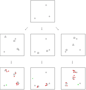
Kang et al. [2011] proposed a hierarchical model based on an independent cluster process to describe the mechanism generating the foci. The model is structured into 3 levels, of which the lowest level, level 1, contains the observations (foci), while higher levels describe the study and population structure respectively. The distinction between singly and multiply reported foci is incorporated into the model.

In the outline of the model below, we occasionally suppress thek index so thatxi

is the set of foci reported in study i, i.e.xi=Skxik.

Figure 3.1 provides a graphical representation of the model. At level 1, we

have foci (Fig. 3.1 bottom, coloured circles). We denote withXi for the underlying

process generating the observations xi in each study. As discussed in Section 2.1,

we can have both multiply and singly reported foci. Thus, Xi consists of two

mechanisms, one generating the multiply reported foci (Fig. 3.1 bottom, red circles) and one that is giving the singly reported foci (Fig. 3.1 bottom, green circles):

Xi=X1i [X0i.

Multiply reported fociX1i can be viewed as an independent cluster process of

points X1i⇠, which are normally distributed around study activation centers ⇠ 2yi

with covariance matrix ⇠ (a random mark attached to every ⇠ 2 yi). That is,

X1i = S

⇠2y_iX1i⇠ and for all ⇠2yi:

X1i⇠ ⇠N(⇠, ⇠). (3.11)

Singly reported foci,X0i, come directly from the population activation centersz as

realisations ofX0i⇣, which are normally distributed around population centers ⇣2z

with covariance matrix ⌃⇣:

X0i⇣ ⇠N(⇣,⌃⇣). (3.12)

To add more flexibility, the model allows for some singly reported foci to not cluster

around any population center, say xi_;. These foci are assumed to arise from a

Poisson processXi_; of constant intensity ✏1:

Xi;|✏1⇠PP(B,✏1). (3.13)

Overall,X0i =

⇣S

⇣₂zX0i⇣

⌘

[Xi_; are the singly reported foci of a study.

At level 2, we have the unobserved study activation centers yi, which are

the locations around which the multiply reported foci of a study cluster. The yi

are realisations of a point processYiand may either cluster around the population

(31)

(Fig. 3.1 middle, triangles). To account for the former, clustered study centers,Yi⇣

are introduced as sets of points normally distributed around population centers⇣2z

with variance matrix ⌃⇣. As for the latter, noise study centers are modelled as a

homogenous Poisson processYi; with intensity✏2. Overall,Yi=⇣S⇣₂zYi⇣

⌘

[Yi;,

where:

Yi⇣ ⇠N(⇣,⌃⇣), (3.14)

and

Yi_;|✏2⇠PP(B,✏2). (3.15)

At the highest level (level 3), we have the population activation centres (Fig.

3.1 top, gray crosses). These are unobserved realisationszof ana priorihomogenous

Poisson processZ of intensity✏3:

Z|✏3⇠PP(B,✏3). (3.16)

Population activation centres are the locations around which study activation centers and singly reported foci scatter. As such, they can be viewed as locations in the brain where an overall population e↵ect exists.

The BHICP can be viewed as a random e↵ects model as it allows for both within-study and between-study variability. Samples from the posterior distribu-tions are obtained via MCMC. Several interesting quantities can be inferred upon such as regions of consistent activations (through the distribution of populations centers), the uncertainty in the location of study centers around the population

centers (through⌃⇣) and the variability of the foci within studies (through ⇠).

A Bayesian nonparametric binary regression model

Yueet al.[2012] use spatial logistic regression for a meta-analysis of emotion studies.

For study iand voxel v, letyi(v) be the binary outcome defined as:

yi(v) = 8 < :

1 at least one focus at voxelv

0 no foci at voxel v . (3.17)

Note that the binary study images {yi(v)}Vv=1 are identical to the MKDA study

mapsMi(v). Logistic regression can be used to model the probability that a voxel

is reported as a focus,pi(v) =_P(yi(v) = 1). It is assumed that:

(32)

+

●●

●

● ● ●

● ●

●

+

●●

● ●●

*

+

● ●

[image:32.595.145.507.174.550.2]

●

Figure 3.1: Realisation of the BHICP model for 3 studies. At level 1 (top) latent

population centres (grey, z) lie. At level 2 (middle) we have centres of multiply

reported foci (black). These come either directly from population centres (squares,

yi) or from background noise (triangles, yi_;). Level 1 (bottom) contains the data

(xi). These are multiply (red,x1

i) or singly (green,x0i) reported foci. Singly reported

foci come either directly from population centres (dots, x0_i_⇠) or from a background

Poisson process (asterisks,x0

(33)

whereH(·) is the link function. The authors use the standard probit and logit link functions.

Spatial correlation is induced through the prior on{z(v)}Vv=1. In particular,

we assume that the process z(v) is an adaptive Gaussian Markov random field

[Yue and Speckman, 2010, aGMRF]. The aGMRF model defines the conditional

distribution of z(v) through a specific dependence with neighbouring voxels. A

significant merit of the method is the inclusion of a local smoothness parameter (v) for the aGMRF. This allows the method to automatically choose the amount of smoothing required depending on the amount of information available.

Authors further introduce a process i(v), an indicator of whether the

out-come variable yi(v) is miscoded; the case i(v) = 1 can either refer to both false

positives, voxels that were falsely found as activated, and false negatives, voxels that

were not reported as foci even though they were activated. The process (v) is not

observed and hence is estimated along with the remaining model parameters. Posterior probabilities of activation at each voxel are obtained through an auxiliary variable MCMC algorithm. Voxels with high posterior probabilities of being reported as foci are more likely to show an e↵ect. A potential drawback of the method is that it can be currently applied only in two dimensions. In three

dimensions, the value of one of the axes is held fixed, for example z = c, while

the model is fitted for all available observations of the formxik = [(xik)1,(xik)2, c].

Authors however, maintain that extending the model to three dimensions is possible.

A hierarchical Poisson/Gamma random field model (HPGRF)

A neuroimaging meta-analysis will typically consider several subtypes of tasks. For example, a meta-analysis of emotion may classify the studies according to experi-ments on “happiness”, “sadness”, “pain”, etc. Yet, the methods described

previ-ously are for a single homogeneous group of studies. Kang et al.[2014] propose a

model that models each type of foci separately, allowing simultaneously for

depen-dence between theJ di↵erent types.

Letxijbe the set of foci reported by studyifor task typej. Suppose thatxij

are realisations of a Cox ProcessXj driven by a random intensity measure ⇤j(d⇠).

Conditional on⇤j(d⇠), Xj are Poisson processes on the brain B:

Xj |⇤j(d⇠)⇠PP(B,⇤j(d⇠)). (3.19)

In other words, we haveJ underlying Cox processes, each one contributing a

(34)

from a convolution of a finite kernel measureKj(d⇠,⇣) and a Gamma Random Field

Gj(d⇣):

⇤j(d⇠) = Z

B

Kj(d⇠,⇣)Gj(d⇣). (3.20)

The model arising from (3.19)-(3.20) is similar to the Poisson/Gamma ran-dom field model of Wolpert and Ickstadt [1998], who first introduced the idea of convolving a Gamma random field with a Poisson process. To introduce dependence

between the di↵erent tasks, it is assumed thatGj(d⇣) are independent realisations

of a Gamma random field with common shape measure G0(d⇣) and inverse scale

parameter :

Gj(d⇣)⇠GRF(G0(d⇣), ). (3.21)

Again,G0(d⇣) is a Gamma random field:

G0(d⇣)⇠GRF(↵(d⇣), 0). (3.22)

An MCMC scheme is used for posterior computation. The HPGRF model

allows for the detection of overall e↵ects based on the posterior intensity G0(d⇣)

or task-specific e↵ects based on⇤j(d⇠). Inference on types with fewer observations

can be done by borrowing information from the remaining types through correlation

under the common base intensityG0(d⇣). A significant benefit of the model is that

it requires the specification of very few hyperparameters.

3.3 Evaluation of existing methods

One of the aims of this dissertation is to evaluate CBMA methods. A head-to-head comparison of existing methodologies is unfeasible, because the statistics described earlier have very di↵erent interpretations. Instead, we examine some characteristics of CBMA methods that show the drawbacks and merits of each. In what follows, we focus on the comparison between kernel-based and model-based methods. In Section 3.3.1 we conduct a series of simulations to study the sensitivity properties of the ALE algorithm that we think characterise other kernel-based methods as well. In Section 3.3.2, we apply the methods for which available software exists on a real dataset and compare the outputs. Finally, in Section 3.3.3 we move to a discussion.

3.3.1 ALE simulation study

(35)

datasets. We perform a simulation study to assess the power properties of the ALE method. In particular, we want to assess how the power of the algorithm evolves with respect to the number of studies in the meta-analysis and whether the method is robust to the inclusion of low quality studies. We choose ALE for three main reasons. Firstly, ALE is currently the most broadly used method for CBMA (based on a PubMed search for ALE, MKDA and SDM). Secondly, a recent review of kernel-based methods [Radua and Mataix-Cols, 2012] reported that the three kernel-kernel-based methods provide qualitatively similar results, thus we expect that our findings are indicative of MKDA and SDM methods as well. Finally, we strongly believe that

the current version of ALE [Eickho↵ et al., 2012] provides the best approximation

to the Monte Carlo test null distribution upon which inference is based.

We create meta-analytic datasets based on the following setup. Each

simu-lated dataset consists ofI studies; of these, Ipare valid while the restI(1 p) are

noise, 0p1. For the valid studies, we assume there exist 8 population centers

around which foci cluster. A valid study detects each population center indepen-dently with probability 0.8. Conditional on detection, a study will report a singly reported focus with probability 0.4, two multiply reported foci with probability 0.35 or three multiply reported foci with probability 0.25. The foci are drawn from a three dimensional Gaussian distribution centered at the corresponding population center. As for the noise studies, we simply sample foci uniformly from the brain mask. The expected number of foci for both valid and noise studies is set to 13, similar to what we found in one of our applications (see Section 4.5).

We use study numbers of I of 20,40,60,80,100 and 120. For a given I we

successively set p = 0,0.05,0.10,0.15, ...,0.95,1. For each distinct combination of

I and p we create B = 1,000 datasets as described above, and apply the ALE

algorithm [Eickho↵ et al., 2012] to each dataset. We use an ↵ = 0.05 FDR

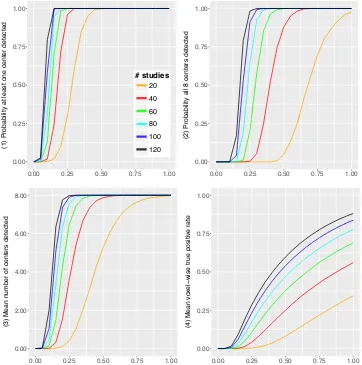
cor-rected threshold to access significance of the ALE statistic images. The following power-related quantities are recorded: 1) the probability that at least one of the 8 population centers is detected; 2) the probability all 8 centers are detected; 3) the mean number of centers detected in 1,000 runs; 4) the mean voxel-wise true positive rate, where “truly” active voxels are defined by the 95% probability spheres around the population centers.

Our findings are summarised in Figure 3.2 where quantities 1 4 are plotted

against the proportion of valid studies. One can observe that all 4 power measures

increase monotonically to their maximal values of 1,1,8 and 1, respectively, as the

(36)

power increases with the proportion of valid studies. Therefore, ALE is a consistent

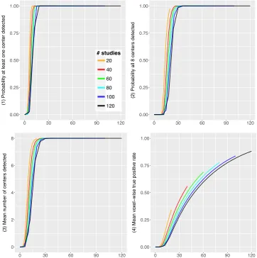
test. In Figure 3.3 we plot quantities 1 4 versus the total number of valid studies,

that is, Ip instead of p. We see that the curves for di↵erent I tend to coincide.

This is a key robustness property of the ALE algorithm: that is, adding pure-noise studies does not degrade power detection.

0.00 0.25 0.50 0.75 1.00

(1) Probability at least one center detected

# studies

20

40

60

80

100

120

0.00 0.25 0.50 0.75 1.00

(2) Probability all 8 centers detected

0.00 2.00 4.00 6.00 8.00

0.00 0.25 0.50 0.75 1.00

(3) Mean n

umber of centers detected

0.00 0.25 0.50 0.75 1.00

(4) Mean v

o

xel

−

wise tr

ue positiv

e r

[image:36.595.138.500.209.574.2]

ate

Figure 3.2: Results of the simulation study. Power properties of the ALE algorithm

are plotted against the proportion of valid studies p. Top left: probability at least

(37)

0.00 0.25 0.50 0.75 1.00

0 30 60 90 120

(1) Probability at least one center detected

# studies

20

40

60

80

100

120

0.00 0.25 0.50 0.75 1.00

0 30 60 90 120

(2) Probability all 8 centers detected

0 2 4 6 8

0 30 60 90 120

(3) Mean n

umber of centers detected

0.00 0.25 0.50 0.75 1.00

0 30 60 90 120

(4) Mean v

o

xel

−

wise tr

ue positiv

e r

[image:37.595.137.499.202.566.2]

ate

Figure 3.3: Results of the simulation study. Power properties of the ALE algorithm

are plotted against the total number of valid studies Ip. Top left: probability at

(38)

3.3.2 Analysis of a real dataset

In this section, we perform a meta analysis of emotion studies that will facilitate the discussion of the next section. The dataset consists of 164 experiments conducted between 1993 and 2005. Eight emotion types appear in the dataset: a↵ective, anger, disgust, fear, happy, mixed, sad and surprise. A total number of 2478 foci is reported with a mean value of foci per study close to 6. The goal of the analysis is to find regions of consistent activation across emotions. Due to the lack of software

availability we only apply MKDA1_{, ALE}2_{, SDM}3 _{and the BHICP}4_{. Since those}

methods can not account for di↵erent task types we treat di↵erent emotions within

an experiment as independent; this results into a total sample size ofI= 437 studies

(contrasts). The same dataset was analysed by Koberet al.[2008], Kanget al.[2011]

and Yueet al.[2012].

The simulation parameters are set as following. For MKDA, we use a kernel

size of r = 10mm, which is also the software default. A total of 10,000 Monte

Carlo datasets are generated under the null hypothesis and used to the threshold

the MKDA statistic imagem(v) at↵= 0.05, FWE corrected. ALE automatically

assigns a kernel size for each study based on the total number of participants and

uses the method of Eickho↵et al.[2012] to calculate the distribution of the statistic

under the null hypothesis. The significance of the statistic image `(v) is accessed

with an FDR corrected ↵ = 0.05 threshold. For SDM we use an isotropic kernel

of 20mm since it is the software default and do 500 Monte Carlo randomisations. For the BHICP we run the MCMC for 120,000 iterations saving once every 100 iterations. This results to a total sample size of 1,200 posterior draws, of which we discard the first 200 a burn-in. We use the same hyperparameter values as in Kang

et al.[2011]. We now summarise the results.

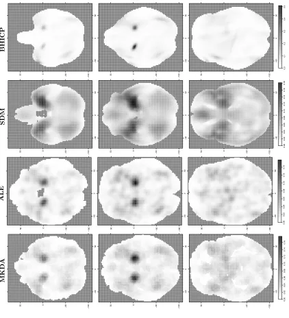
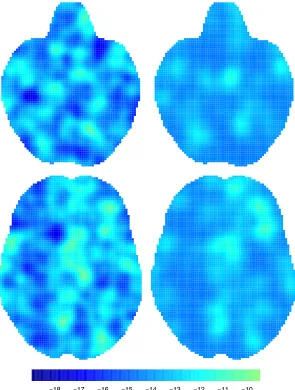
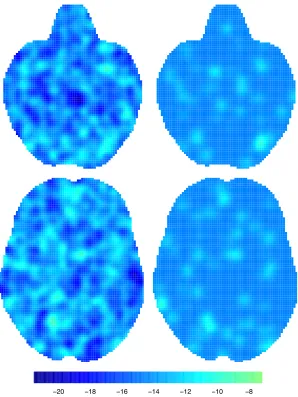
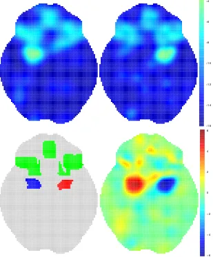
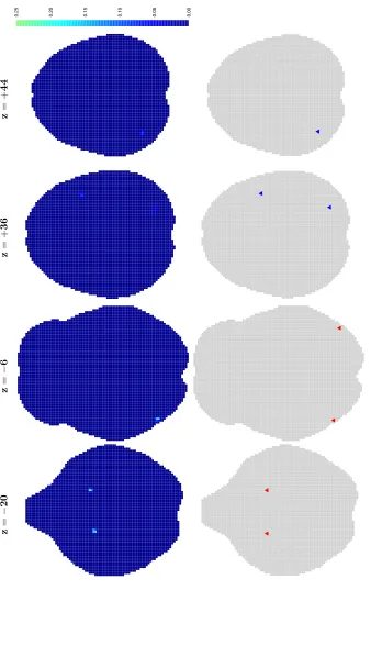
Figure 3.4 shows statistic images obtained from the four methods considered,

conditional on several values of thez dimension. Note that for the BHICP we show

only the study activation process intensity function. We see that all of the methods provide qualitatively similar results. More specifically, the regions of the brain that are mostly engaged in emotion processing are the right and left amygdala (Fig. 3.4, top and middle row). This finding is consistent with previous analyses of the same

dataset [Koberet al., 2008; Kanget al., 2011; Yueet al., 2012] as well as results of

previous studies [Phelps and LeDoux, 2005; Costafredaet al., 2008]. Other regions

1_{http://wagerlab.colorado.edu/files/tools/meta-analysis.html}

2_{http://www.brainmap.org/ale/}

3_{http://www.sdmproject.com/software/}

4

(39)

(40)

[image:40.595.91.513.183.647.2]

(41)

3.3.3 Discussion

The meta-analysis of emotions suggests that the outputs obtained from model-based methods are qualitatively similar to those obtained from kernel-based methods. Nev-ertheless, the two approaches are fundamentally di↵erent.

In terms of computational time, it is clear that kernel-based methods outper-form model-based methods (with the exception of SDM). For the emotion dataset used in the illustration of Section 3.3.2 ALE required approximately 15 minutes to run and MKDA required around 3 hours for 10,000 Monte Carlo replications. On the contrary, the BHICP model took roughly 16 hours for 120,000 MCMC

itera-tions, Kanget al.[2014] needed 20 hours to complete the analysis and it is yet not

possible to run the spatial binary regression model on the full brain.

Apart from running time, one needs to consider the ease of implementa-tion. On the one hand, software for kernel-based methods can be applied to any dataset and will produce a pair of brain images: one with the value of the statistic

and one containing the correspondingp-values. That results into a very automated

procedure: one can directly compare the two images and see which voxels where significant and which were not. On the other hand, it is not straightforward to implement an MCMC scheme for one of the model-based methods. Prior specifica-tions that are suitable for one dataset may be completely inappropriate for another. Further, it is not possible to know in advance how many iterations are required for the MCMC algorithm to converge, and convergence needs to be assessed as well. Overall, it may not seem appealing for a neuroimaging practitioner to adopt model-based methods and this explains why kernel-model-based methods are generally preferred in the outstanding majority of the analyses.

Nevertheless, despite the ease of implementation kernel-based methods allow for very limited inferences. First of all, kernel-based methods cannot be viewed

as spatial models but are instead massively univariate approaches (MUA). This

means that any inference is done voxel-by-voxel a no argument can be done for a

priori defined groups of voxels or the entire brain. As an example, with kernel-based methods it is not possible to infer the total number of foci in a study; in fact, analyses condition on the total number of foci in a study. For model-based methods based on point processes such as the BHICP, the expected number of foci can be obtained by integrating the intensities over the brain. Further, MUA do not account for the spatial correlation and hence there is no borrowing of information across voxels. This leads to poor spatial precision as can be seen in Figure 3.4 where the BHICP statistic is more concentrated compared to the kernel-based methods.

(42)

standard errors given and therefore it is not possible to quantify the uncertainty for the e↵ect estimate through confidence intervals, which in turn may result to misleading conclusions. For example, in Section 3.3.1 we found that power prop-erties of ALE do not degrade with the inclusion of poor quality studies (see Fig. 3.3). However, since inferences remain unchanged, it is not possible to distinguish between cases with strong signal (few poor quality studies) and weak signal (many poor quality studies). Note that this is a fixed e↵ects model property where a small proportion of the data drives the inference. Model-based methods tackle this through the standard errors obtained directly from the posterior distribution of any parameters of interest; when the signal is strong there is small variability in the pos-terior whereas when the signal is weak the variability is higher. Finally, kernel-based methods provide no adequate justification for the choice of kernel size parameter (r

for MKDA and for ALE, SDM). Typically, its value is specified based on previous

studies rather than being estimated from the data, and it remains constant across the brain regardless of the amount of smoothing required in each region. A bad choice of the kernel size can potentially a↵ect the results, though. For example, in Figure 3.4 we see that in the statistic image of SDM the clusters appear to be bigger, because we have used a larger kernel size compared to the other kernel-based

methods. Yue et al.[2012] automatically choose the amount of smoothing require

introducing an extra smoothness parameters to their aGMRF.

Several other quantities of interest can be obtained from model-based

meth-ods. For the BHICP model it is possible to derive (1 ↵)% credible ellipses for both

population and study activation centers thus returning an estimate of within-study and between study-variability as in a random e↵ects meta-analysis model. By

intro-ducing the latent process (v), Yueet al.[2012] estimate the probability of a voxel

being miscoded. In the HPGRF model, the authors provide correlation estimates between the di↵erent emotions. All these quantities can not be obtained by any of the kernel-based methods.

Finally, the Bayesian framework upon which model-based methods are build facilitates the construction of predictive distributions over new studies. This helps

producing the so-calledreverse inferences[Poldrack, 2011], a topic of growing

inter-est in the fMRI community. Traditionally, fMRI studies produceforward inferences:

(43)

case the researcher would want an estimate of the probability that the data arose

from a population of emotion studies. Kang et al. [2014] show that classification

based on the HPGRF model outperforms a naive classifier based on MKDA. This result suggests spatial models can captures information in the data that cannot be captured by a MUA.

For all these reasons, we believe that model-based methods have significant merits compared to kernel-based methods. However there are several still open problem for model-based methods and CBMA in general. We discuss those in the following section.

3.4 Open problems

There are currently some aspects of CBMA that are being overlooked by both

model-based and kernel-based methods. The most important is publication bias.

Publication bias happens when the studies to which researchers have access are not a representative subset of the total population of studies. For example, one special

case of publication bias is thefile drawer where studies with significant findings are

more likely to get published. If present, publication bias can a↵ect the outcome of a meta-analysis and lead to false conclusions. In the field of fMRI there is evidence

for the existence of publication biases [David et al., 2013] but there has been no

attempt to quantify the e↵ect these biases may have on our meta-analysis estimates. In Chapter 6 we use a simple model to estimate the number of missing studies due to the file drawer in CBMA. Nevertheless, there is still a need to adjust existing methods (or develop new ones) to account for the presence of publication bias.

Another still open problem is meta-regression. Meta-regression extends the simple meta-analysis model to account for study characteristics. When available, such information can improve the fit of a model and give better insights on the data. In CBMA several study characteristics are typically recorded when that data are gathered but it is not yet a commonplace to use this information in meta-analyses. In Chapter 4 we outline a model that uses study characteristics as explanatory variables thus introducing the notion of meta-regression in CBMA.

One interesting problem is how CBMA can be jointly modelled with image data from new fMRI studies. Currently there are no models that connect the image data with the foci and hence it is not possible to use the former as prior information

or investigate if the two agree. In Chapter 5 we propose a model for fMRIT statistic

data that uses CBMA data as prior information.

(44)

connectivity refers to the dependency between one or more regions of the brain. In CBMA functional connectivity is implied by co-activation, that is, when two

regions consistently report activations. In a recent work, Xue et al. [2014] use a

Point process modelling of coordinate based meta analysis neuroimaging data

warwick.ac.uk/lib-publications

A Thesis Submitted for the Degree of PhD at the University of Warwick

Permanent WRAP URL:

http://wrap.warwick.ac.uk/87635

Copyright and reuse:

This thesis is made available online and is protected by original copyright.

Please scroll down to view the document itself.

Please refer to the repository record for this item for information to help you to cite it.

Our policy information is available from the repository home page.

Point process modelling of

coordinate-based meta-analysis

neuroimaging data

by

Pantelis Samartsidis

Thesis

Submitted to the University of Warwick

for the degree of

Doctor of Philosophy

Department of Statistics

Contents

List of Tables

List of Figures

Acknowledgments

Declarations

Abstract

Chapter 1

Introduction

Chapter 2

Background

2.1

Neuroimaging background

2.1.1

Limitations of individual studies and meta-analysis

2.2

Spatial point processes background

Chapter 3

The coordinate-based

meta-analysis of fMRI data: a

review

3.1

Introduction

3.2

CBMA methods

3.2.1

Kernel-based methods

3.2.2

Model-based Methods

+

+

+

+

+

+

+

+

+

+

+

+

+

+

+

+

+

+

*

+

+

+

3.3

Evaluation of existing methods

3.3.1

ALE simulation study

3.3.2

Analysis of a real dataset

3.3.3

Discussion

3.4

Open problems