Oscillations in stellar superflares

warwick.ac.uk/lib-publications

Original citation:

Balona, L. A., Broomhall, Anne-Marie, Kosovichev, A., Nakariakov, V. M., Pugh, C. E. and Van

Doorsselaere, Tom. (2015) Oscillations in stellar superflares. Monthly Notices of the Royal

Astronomical Society, 450 (1). pp. 956-966.

Permanent WRAP URL:

http://wrap.warwick.ac.uk/78692

Copyright and reuse:

The Warwick Research Archive Portal (WRAP) makes this work by researchers of the

University of Warwick available open access under the following conditions. Copyright ©

and all moral rights to the version of the paper presented here belong to the individual

author(s) and/or other copyright owners. To the extent reasonable and practicable the

material made available in WRAP has been checked for eligibility before being made

available.

Copies of full items can be used for personal research or study, educational, or not-for profit

purposes without prior permission or charge. Provided that the authors, title and full

bibliographic details are credited, a hyperlink and/or URL is given for the original metadata

page and the content is not changed in any way.

Publisher’s statement:

This is a pre-copyedited, author-produced PDF of an article accepted for publication in

Monthly Notices of the Royal Astronomical Society following peer review. The version of

record Balona, L. A., Broomhall, Anne-Marie, Kosovichev, A., Nakariakov, V. M., Pugh, C. E.

and Van Doorsselaere, Tom. (2015) Oscillations in stellar superflares. Monthly Notices of the

Royal Astronomical Society, 450 (1). pp. 956-966. is available online at:

http://dx.doi.org/10.1093/mnras/stv661

A note on versions:

The version presented here may differ from the published version or, version of record, if

you wish to cite this item you are advised to consult the publisher’s version. Please see the

‘permanent WRAP url’ above for details on accessing the published version and note that

access may require a subscription.

arXiv:1504.01491v1 [astro-ph.SR] 7 Apr 2015

Oscillations in stellar superflares

L.A. Balona

, A.-M. Broomhall

, A. Kosovichev

, V. M. Nakariakov

,

C.E. Pugh

, T. Van Doorsselaere

1_{South African Astronomical Observatory, P.O. Box 9, Observatory 7935, South Africa}

2_{Centre for Fusion, Space and Astrophysics, Department of Physics, University of Warwick, CV4 7AL, UK} 3_{Institute of Advanced Studies, University of Warwick, CV4 7HS, UK}

4_{New Jersey Institute of Technology, Newark, NJ 07103, USA}

5_{Central Astronomical Observatory at Pulkovo of the Russian Academy of Sciences, St Petersburg 196140, Russia} 6_{Centre for mathematical Plasma Astrophysics, Department of Mathematics, KU Leuven,}

Celestijnenlaan 200B bus 2400, B-3001 Leuven, Belgium

ABSTRACT

Two different mechanisms may act to induce quasi-periodic pulsations (QPP) in whole-disk observations of stellar flares. One mechanism may be magneto-hydromagnetic (MHD) forces and other processes acting on flare loops as seen in the Sun. The other mechanism may be forced local acoustic oscillations due to the high-energy particle impulse generated by the flare (known as ‘sunquakes’ in the Sun). We analyze short-cadenceKeplerdata of 257 flares in 75 stars to search for QPP in the flare decay branch or post-flare oscillations which may be attributed to either of these two mechanisms. About 18 percent of stellar flares show a distinct bump in the flare decay branch of unknown origin. The bump does not seem to be a highly-damped global oscillation because the periods of the bumps derived from wavelet analysis do not correlate with any stellar parameter. We detected damped oscillations covering several cycles (QPP), in seven flares on five stars. The periods of these oscillations also do not correlate with any stellar parameter, suggesting that these may be a due to flare loop oscillations. We searched for forced global oscillations which might result after a strong flare. To this end, we investigated the behaviour of the amplitudes of solar-like oscillations in eight stars before and after a flare. However, no clear amplitude change could be detected. We also analyzed the amplitudes of the self-excited pulsations in twoδScuti stars and one γ Doradus star before and after a flare. Again, no clear amplitude changes were found. Our conclusions are that a new process needs to be found to explain the high incidence of bumps in stellar flare light curves, that flare loop oscillations may have been detected in a few stars and that no conclusive evidence exists as yet for flare induced global acoustic oscillations (starquakes).

Key words: stars: flare – stars: activity

1 INTRODUCTION

Photometric observations from the Keplerspacecraft have revealed flares in a considerable number of stars. These oc-cur not only in cool M dwarfs, but in K, G, F and A stars as well. The numbers of B stars observed by Kepler are too few to allow detection of flares. Because even the weak-est visible stellar flares are thousands of times more ener-getic than a large solar flare, these are often called “super-flares”. Walkowicz et al. (2011) were the first to identify 373 flare stars out of ≈ 23000 cool dwarfs in the Kepler field.

Subsequently, Maehara et al. (2012) discovered 148 solar-type stars with superflares. More recently, Shibayama et al. (2013) found superflares on 279 G dwarfs. Balona (2012) and Balona (2013) discovered several A stars with superflares

which cannot be attributed to flares in a cool companion. It appears that A stars may have spots and flares in spite of the lack of significant convection. In fact, the incidence of flares on A stars is not much lower than in G and F stars (Balona 2015). In these hot stars the magnetic field may be a result of the Tayler instability in a differentially-rotating star (Spruit 2002; Mullan & MacDonald 2005).

Even the strongest solar flares are barely detected in space observations of total solar irradiance and the Sun would not be detected as a flare star byKepler. It is thought that solar flares arise from the energy released by magnetic reconnec-tion. Although superflares are typically 106_{times more} ener-getic than large solar flares, it is possible that the magnetic reconnection model may still apply (Shibata et al. 2013).

Nearly all Keplerphotometry has been obtained with 30-min long-cadence (LC) exposures, which means that only flares which have a long duration can be detected. A few thousand stars were observed with 1-min short-cadence (SC) exposures, though only for a relatively short time. Whereas LC data are nearly continuous over the four-year time span of Keplerobservations, the SC data cover typically only a few months for any star. The advantage of SC data is that it allows flares of short duration to be detected. Balona (2015) discovered 3140 flares in 209 stars of all spectral types ob-served in SC mode. In this paper the flare in a particular star is identified by its sequence number. For example 002300039-028 is the 28-th flare in KIC 2300039 listed in the catalogue of Balona (2015).

We know that quasi-periodic pulsations (QPP) of coro-nal loops occur in some solar flares (Nakariakov & Melnikov 2009; Nakariakov et al. 2010). The mechanism giving rise to QPP is not fully understood at present. One possibility pointed out by McLaughlin et al. (2012) is that of oscilla-tory reconnection. The behaviour of oscillaoscilla-tory reconnection is similar to a damped harmonic oscillator and may play a role in generating QPP.

Analysis of QPP can provide information on the flare coronal environment and magnetic field strength by the use of seismology (Kupriyanova et al. 2013). How-ever, solar flare QPP are only observed in Hα, extreme UV lines and in radio and X-ray and gamma-ray ob-servations. There are no recorded observations of QPP in white-light solar flares. The reported optical observa-tions of QPP in stellar flares (Rodono 1974; Zhilyaev et al. 2000; Mathioudakis et al. 2006; Contadakis et al. 2010; Qian et al. 2012; Anfinogentov et al. 2013), which have pe-riods ranging from a few seconds to tens of minutes, are whole-disk essentially white-light observations. They can-not therefore be directly compared with solar flare QPP. It is also far from certain if white-light stellar flares are gener-ated in the same way as solar flares.

Solar and stellar QPP have previously been used to pro-vide estimates for several flare parameters. An example of QPP with large amplitude and duration in a solar flare ob-served in X-ray and microwave radio bursts in described by Kane et al. (1983). More recently, Van Doorsselaere et al. (2011) used X-ray observations of two oscillation modes in a single solar flare to estimate the plasma-beta and the density contrast of the flaring loop. The wave mode number was also estimated from the observed periods. Anfinogentov et al. (2013) analyzed the oscillatory signal in the decay phase of the U-band light curve of a flare in the dM4.5e star YZ CMi. The observational signature is typical of the longitudinal os-cillations observed in solar flares at extreme ultraviolet and radio wavelengths and is associated with standing slow mag-netoacoustic waves. They therefore suggest that the QPP in this stellar superflare may be of a similar nature to so-lar QPP. A well pronounced QPP has been reported dur-ing an very energetic flare on the RS CVn binary II Peg

(Mathioudakis et al. 2003). The QPP has a long period lead-ing to the peak.

The dynamic impact in the photosphere caused by a solar flare is called a “sunquake”. The resulting helio-seismic waves are observed as expanding circular ripples on the solar surface, which can be detected in Doppler-grams and as a characteristic ridge in time-distance dia-grams (Kosovichev & Zharkova 1998; Kosovichev 2006), or by calculating the integrated acoustic emission (Donea et al. 1999; Donea & Lindsey 2005). These flare-excited oscilla-tions are mostly local seismic waves. While the theory pre-dicts that global acoustic waves should also be excited, their amplitudes are thought to be significantly lower than the amplitudes of stochastically excited oscillations (Kosovichev 2009). Most of the emitted acoustic energy of sunquakes is above the acoustic cut-off frequency of the Sun.

Karoff & Kjeldsen (2008) concluded that global high-frequency solar acoustic waves have larger amplitudes af-ter some solar flares, a finding confirmed by Kumar et al. (2010). However, Richardson et al. (2012) found that a de-crease in acoustic power after a solar flare is just as likely as an increase. This is perhaps not surprising because the effect of the impulse on a global seismic mode depends on the location and time of the impulse. The effect of the im-pulse is therefore expected to increase the amplitude of some modes and decrease the amplitude in other modes. The re-sult should be a higher variation in amplitude distribution after a flare.

In the case of the vastly more powerful stellar super-flares, the impact on the star may be much greater and it is conceivable that these forced oscillations may be ob-served. This idea has been discussed by Karoff (2014) and Kosovichev (2014) inKeplerphotometry of solar-like stars. Karoff found no significant enhancement of the energy in the post-flare acoustic spectra relative to the pre-flare en-ergy. However, a larger variability between the energy in the high-frequency part of the post- and pre-flare acoustic spec-tra was found compared to specspec-tra taken at random times. This may be a result of the increased dispersion in acoustic energy discussed above.

In spite of the very large differences in energy and op-tical emission between solar and stellar flares, the possibil-ity exists that the physical mechanisms for QPP could be very similar. In this paper we investigate QPP inKepler su-perflares because this could provide additional clues to the nature of stellar flares. We also investigate the possible oc-currence of starquakes as a result of a superflare and search for excitation of global acoustic oscillation modes in the pe-riodogram. These investigations are only possible due to the superb precision of theKeplerdata, a unique resource which is unlikely to be equaled for many years to come.

2 DATA AND ANALYSIS TECHNIQUE

Our analysis is based on the 3140 flares in 290 stars observed in SC mode as described in Balona (2015). Out of these 3140 flares, we selected 257 flares in 75 stars with sufficiently high signal-to-noise (S/N) to be suitable for detecting possible flare oscillations.

0 20 40 60

-100 0 100 200 300 400 500 600 700

ppt

002852961-004

-10 -5 0 5 10

ppt

Period (min)

0 50 100 150 200 250 300

Time (min) 0

50 100 150 200

0 10 20

-50 0 50 100 150 200 250

ppt

006437385-005

0 5

ppt

Period (min)

0 20 40 60 80 100

Time (min) 0

50 100 150

0 10 20 30

-50 0 50 100 150 200

ppt

008081482-009

-5 0 5

ppt

Period (min)

0 20 40 60 80 100

Time (min) 0

50 100 150

0 10 20 30

-50 0 50 100 150 200 250 300 350

ppt

011551430-017

-2 0 2 4

ppt

Period (min)

0 20 40 60 80 100

Time (min) 0

50 100

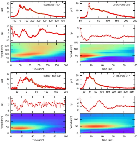
Figure 1.Examples of four flares showing bumps on the decay branch. The top panel shows the flare light curve and fitted polynomial. The middle panel shows the decay branch with polynomial removed, with time measured from the time of maximum flare intensity. The bottom panel shows the wavelet spectrum as a function of time relative to the time of maximum flare intensity. The intensity is measured in parts per thousand (ppt). The KIC number and the flare identifier from the catalogue of Balona (2015) is shown.

We found that a polynomial of the form log(y) =a0+a1t+a2t2+a3t3. . .

generally provides a good fit to the flare decay intensity. Here

tis the time measured from flare maximum andyis the flare intensity. In nearly every case, a cubic polynomial was used. The polynomial was removed and the residuals plotted as a function of time. In about 18 percent of theKeplerflares, one or more bumps are present in the decay branch. A low-degree polynomial does not adequately remove these features. In these cases, the large-scale structures can be removed by applying a suitable filter to the data, as described below.

Flare loop oscillations (QPP) are usually seen as

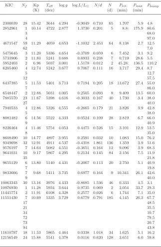
Table 1.Physical parameters for stars in which one or more bumps are visible in the flare light curve. The second column,Nf, is an

identifier for the flare, which is theNf-th flare for the particular star in the catalogue of Balona (2015). TheKeplermagnitude,Kp,

effective temperature,Teff (K) and surface gravity, logg, is taken from theKepler Input Catalogue (KIC). The luminosity,L/L⊙ is

derived from the effective temperature and radius listed in the KIC. The average number of flares per day,N/d, and the total number of

observed flares,N, are shown. The rotation period,Prot(d), are from Balona (2015).Pmaxis the expected period of solar-like oscillations

(min). The last column is the derived period from wavelet analysis.

KIC Nf Kp Teff logg logL/L⊙ N/d N Prot Pmax Pbump

(K) (dex) (d) (min) (min)

2300039 28 15.42 3644 4.294 -0.9049 0.710 65 1.707 5.9 4.8

2852961 1 10.14 4722 2.877 1.3730 0.201 5 8.8: 175.9 80.6

3 68.0

4 97.0

4671547 59 11.29 4059 4.653 -1.1032 2.453 64 8.138 2.7 12.5

62 7.0

5475645 3 11.20 5336 4.654 -0.3709 0.059 6 7.452 3.1 9.2

5733906 2 11.83 5241 3.688 0.6933 0.238 7 0.719 28.6 5.5

5952403 2 6.96 5037 3.001 1.5178 0.012 2 45.28: 136.5 110.2

6205460 4 12.74 5242 3.677 0.7067 0.111 16 3.717 29.4 8.7

5 12.7

12 57.5

6437385 5 11.53 5401 3.713 0.7194 0.205 18 13.672 27.4 55.0

7 86.0

6548447 2 12.88 5031 4.005 0.2505 0.093 8 9.409 13.5 60.0

7885570 23 11.67 5398 4.616 -0.3033 0.167 40 1.730 3.4 38.0

27 40.0

7940533 4 12.86 5326 4.555 -0.2665 0.179 21 3.826 3.9 42.8

5 38.0

8081482 6 14.56 5522 4.333 0.0524 0.109 28 2.819 6.7 66.0

9 40.9

8226464 4 11.46 5754 4.053 0.4475 0.526 15 3.101 12.9 53.5

8 35.0

8608490 10 14.77 4897 3.955 0.2591 0.032 10 1.083 15.0 76.2

9349698 32 12.91 4911 4.537 -0.4318 1.861 136 1.359 3.9 51.6

9576197 7 14.64 5082 4.551 -0.3651 0.164 12 9.096 3.9 68.3

9641031 10 9.17 5867 4.295 0.2134 0.145 84 2.156 7.5 11.9

35 21.8

9655129 6 13.80 5140 4.431 -0.2067 0.113 20 2.750 5.1 40.9

7 19.8

9833666 7 9.68 5411 3.735 0.6977 0.164 9 10.341 26.1 42.6

9 40.0

10063343 30 13.16 3976 4.433 -0.8685 1.536 46 0.333 4.5 3.1

10976930 1 11.28 5934 3.644 0.9735 0.069 2 2.054 33.7 29.3

11445774 2 11.91 6108 4.328 0.2577 0.026 6 1.744 7.1 35.0

11551430 7 10.69 5335 3.729 0.6779 0.791 185 4.145 26.3 67.7

17 48.5

21 35.5

34 10.7

72 79.5

73 20.7

94 43.8

11610797 18 11.53 5865 4.464 0.0338 1.018 34 1.625 5.1 16.2

12156549 24 15.88 5541 4.378 0.0116 0.620 128 3.651 6.0 59.8

as a function of time. This is conveniently accomplished by a greyscale representation of the amplitude in a period–time diagram.

Forced global acoustic oscillations caused by a flare im-pulse are expected to be seen several hours after the flare and with a decay time of perhaps a few days. For detect-ing such oscillations we use standard periodogram analysis

0 100 200

-20 -10 0 10 20 30 40 50

ppt

002300039-028

-20 0 20

ppt

Period (min)

0 10 20 30 40 50

Time (min) 0

5 10

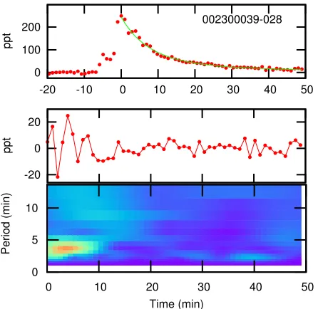
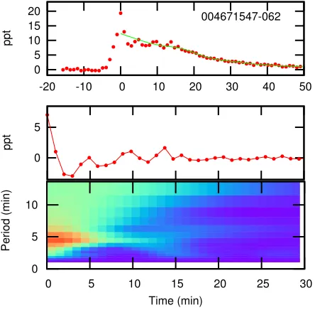
Figure 2.The top panel shows the flare light curve and fitted spline curve. The second panel shows the decay branch with fitted curve removed. The third panel shows the wavelet spectrum.

0 20 40 60 80

-20 -10 0 10 20 30 40 50

ppt

003128488-017

-5 0 5 10

ppt

Period (min)

0 5 10 15 20 25

Time (min) 0

5 10

Figure 3.The same as Fig. 2.

3 FLARES WITH BUMPS IN THE LIGHT CURVE

Of 257 stellar flares selected because of their very high S/N, 47 flares (i.e. 18 percent) show obvious structures (i.e. bumps) in the flare decay light curve. A further 14 percent show a distinct change in the rate of decay (Balona 2015). Examples of flare light curves showing bumps are shown in Fig. 1. One possible reason for such bumps is that two flares occur by chance within the same small interval. One can estimate the chances of such an occurrence by measuring the mean flare rate during a suitable interval. The typical duration of a flare is about one hour. The star with the max-imum flare rate produces, on average, one flare every 10 hr

0 5 10 15 20

-20 0 20 40 60

ppt

004671547-059

-1 -0.5 0 0.5 1

ppt

Period (min)

0 10 20 30 40

Time (min) 0

5 10

Figure 4.The same as Fig. 2.

orx= 0.1 flare hr−1_{. The probability,P, that two flares will} occur in the interval of one hour follows a Poisson distri-bution and is P = x2

2!e

−x _{= 0.005. This is an upper limit}

considering the fact that we have chosen the maximum flare rate. In some stars (e.g. KIC 11551430) there are many flares with bumps. The probability of such an occurrence, assum-ing that what we are seeassum-ing is just a superposition of two or more practically simultaneous flares, is negligible. Hence there must be a physical process involved in producing the bumps. One such process could be sympathetic flaring where one solar flare may trigger another flare (Moon et al. 2002). Both bumps and changes in rate of decay can be mod-eled as QPP with a rapid decay rate. In Fig. 1 the polyno-mial fit to the decaying branch, and the wavelet spectra are shown. Wavelet analysis of 47 “bump” flares in 30 stars in-dicates that significant power is present at a certain period. If we are to make progress in understanding this relatively common phenomenon, the “period” derived in this may offer some clue as to the nature of the bumps.

If we assume that the bump is due to a highly-damped global acoustic mode, for example, one may expect the pe-riod to be correlated with some stellar parameter or combi-nation of parameters. Solar-like modes in stars are excited because their periods are similar to the typical turn-over period of a convective cell and below the acoustic cut-off frequency. As a result, the frequency of maximum ampli-tude, νmax is related to the stellar parameters as follows (Brown et al. 1991; Kjeldsen & Bedding 1995):

νmax≈νmax⊙

M/M⊙

(R/R⊙)2

p

Teff/Teff⊙

,

where the solar value for the frequency of maximum am-plitude is νmax⊙ = 3120µHz, while M/M⊙, R/R⊙ and

Teff/Teff⊙ is the stellar mass, radius and effective

temper-ature relative to the Sun.

0 5 10 15 20

-20 -10 0 10 20 30 40 50

ppt

004671547-062

0 5

ppt

Period (min)

0 5 10 15 20 25 30

Time (min) 0

5 10

Figure 5.The same as Fig. 2.

0 5 10

0 50 100 150

ppt

011551430-021

-1 0 1

ppt

Period (min)

0 20 40 60 80 100

Time (min) 0

10 20

Figure 6.The same as Fig. 2.

cut-off frequency is proportional toνmax, one may expect a correlation between the bump period and Pmax = 1/νmax. The value ofPmax, as calculated from loggandTeff, is shown in Table 1.

As shown in Table 2, the flare bump period (Pbump) can vary widely even in the same star. We can find no correla-tion between this period and Pmax. In fact, no correlation between these timescales and any stellar parameter can be found. It seems that the structures on the decaying branch of the flare, whatever their cause, cannot be attributed to highly-damped impulsively excited global acoustic oscilla-tions. It is still possible that these may be highly-damped flare loop oscillations, but there is no evidence that can be used in support of this notion either. However, the similarity of the observed decaying QPP in stellar superflares, and of

the standing oscillations observed in hot coronal solar flare loops (e.g. Wang 2011; Kim et al. 2012) indicates the pos-sible similarity of the physical processes involved, despite differences in emission spectrum.

4 RAPID OSCILLATIONS

A polynomial fit to the flare decay branch is no longer ad-equate to enhance the visibility of possible oscillations with periods of only a few minutes. We found a segmented spline fit to be adequate for this purpose. In this method, a number of evenly spaced points are selected in the decay branch of the flare light curve. The mean intensity in the neighbour-hood of each point is found. A spline fit is calculated using the time and mean intensities at these points and the fit re-moved from the data. It is important to choose the interval between the segments carefully. If the interval is too small, possible oscillations with periods longer than this interval will not be detected because less than one period will be sampled. On the other hand, if the interval is too long, then the spline interpolation is no longer an adequate fit and the residuals may be contaminated by spurious long-period sig-nals. We found that a choice of 10–15 min was appropriate for the interpolation sampling interval in most cases. We have also tried other methods for trend removal, such as temporal smoothing, but this did not significantly influence the detected periods.

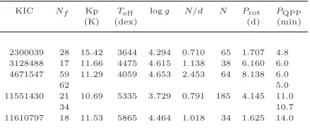
We carefully examined all 257 flares without finding any obvious QPP in the majority of flares. We did not find any cases where QPP begins before the time of flare maximum. This may be due to the long sample time of 1 min and the steep rising branch which which would make such a detec-tion difficult. Evidence for damped oscilladetec-tions after flare maximum is, however, present in the few flares shown in Figs. 2–8. The stellar parameters for these stars are shown in Table 2. Most of these flares also appear in Table 1; other stars in this table do not show more than a single bump.

Gruber et al. (2011) tested the apparent QPP of four bright solar flares observed in gamma rays using classical periodogram analysis, but found that these oscillations were not intrinsic to the flares. Similarly, Vaughan (2010) applied Bayesian statistics to apparent QPP in some Seyfert galax-ies and also found that these were not significant. The dif-ficulty is that the underlying noise in the periodogram is not ‘white’ (i.e., independent of frequency) but ‘red’ (i.e. in-creases towards low frequencies). This variation of noise with frequency needs to be taken into account in any analysis of significance. Because white noise is usually assumed the sig-nificance of QPP has generally been overestimated. This is further illustrated by recent work by Inglis et al. (2015) who investigated supposed QPP in a selection of solar flares from a variety of sources as well as QPP in some optical stellar flares. They found that for all except one event tested, an explicit oscillation is not required in order to explain the observations. Instead, the flare signals are adequately de-scribed as a manifestation of a power law in the Fourier power spectrum, rather than a direct signature of oscillat-ing components or structures.

0 10 20 30 40

0 50 100 150 200 250

ppt

011551430-034

-1 0 1

ppt

Period (min)

0 10 20 30 40 50 60

Time (min) 0

10 20

Figure 7.The same as Fig. 2.

0 10 20 30

0 50 100 150

ppt

011610797-018

-2 0 2

ppt

Period (min)

0 20 40 60 80 100

Time (min) 0

10 20

Figure 8.The same as Fig. 2.

not claim that the oscillating signals seen in Figs. 2–8 are necessarily real. We merely wish to illustrate that QPP in theKeplerflares, if it exists, is not common.

While QPP is a useful diagnostic tool for flares on the Sun, it cannot be used for stellar flares without some un-derlying assumptions. In the Sun one can image the flare, so that the loop length is known. Very often, other parame-ters, such as the plasma temperature, can also be quite well estimated. For stellar flares, however, we only have the pe-riod and decay time of the QPP, so the information that can be extracted is severely limited. Zaitsev & Stepanov (1982) and Roberts et al. (1984) showed that for a simple cylin-drical magnetic flux tube, several types of magneto-acoustic wave modes are possible: the slow (acoustic) mode, the fast kink and the fast sausage modes. These are all observed in

Table 2.Physical parameters for stars in which a damped oscilla-tion (QPP) is visible in the flare light curve. The second column,

Nf, is an identifier for the flare. TheKeplermagnitude,Kp,

effec-tive temperature,Teff(K) and surface gravity, logg, is taken from

theKepler Input Catalogue(KIC). The average number of flares

per day,N/d, and the total number of observed flares, N, are

shown. The variability type and the rotation period,Prot(d), are

from Balona (2015). The last column is the period (min) derived from wavelet analysis.

KIC Nf Kp Teff logg N/d N Prot PQPP

(K) (dex) (d) (min)

2300039 28 15.42 3644 4.294 0.710 65 1.707 4.8 3128488 17 11.66 4475 4.615 1.138 38 6.160 6.0 4671547 59 11.29 4059 4.653 2.453 64 8.138 6.0

62 5.0

11551430 21 10.69 5335 3.729 0.791 185 4.145 11.0

34 10.7

11610797 18 11.53 5865 4.464 1.018 34 1.625 14.0

solar flux tubes and solar flare loops. For a standing oscil-lation in a loop, the loop lengthL is given byL=jcP/2, whereP is the oscillation period,j the parallel mode num-ber andcthe appropriate wave speed. The waves with the longest periods, which are those of interest to us due to the 1-min cadence of theKeplerdata, are the slow modes. For slow modes,cis the tube speed,ctwith

1

c2

t

= 1

c2

s

+ 1

c2

A ,

where cs is the sound speed and cA is the Alfv´en speed.

Since the Alfv´en speed in the coronal loops is considerably larger than the sound speed, we assumec≈cs.

The unknown values ofj, c and L render the extrac-tion of any meaningful physics impossible at this stage. We also note that the above description applies to a low-density plasma environment as occurs in a typical solar coronal flare loop. Stellar flares emit in a continuum and the physical process is likely to be different from that of solar flares even if the energy source, magnetic reconnection, is the same. However, these parameters are contained in the characteris-tic parameters of the decay phase of the flare, the damping time of the oscillations, intensity of the flare, and other ob-servables and, in principle, can be extracted from the data when a sufficiently detailed model becomes available.

5 FLARES IN STARS WITH SOLAR-LIKE OSCILLATIONS

0 5 10 15

250 300 350 400

Frequency (µHz)

12307366 0

10 20 30

40 50 60 70 80 90 100 110

7944142 0

0.5 1

600 800 1000 1200 1400 1600

7940546 0

0.5 1

1200 1400 1600 1800 2000 2200

Amplitude (ppm) 7206837

0 1 2 3

800 1000 1200 1400 1600

6442183 0

2 4

400 600 800 1000

5108214 0

5 10

1400 1600 1800 2000 2200

4554830 0

5 10

40 60 80 100

3430868

Figure 9.Periodograms of flare stars with solar-like oscillations.

Table 3.Parameters for flare stars with solar-like oscillations.

KIC Kp Teff logg logL/L⊙ N/d N Prot

(K) (dex) (d)

3430868 8.13 4729 4.584 -0.5864 0.203 6

-4554830 10.33 5317 4.314 -0.0051 0.039 1 14.602

5108214 7.83 5663 3.857 0.6404 0.028 8

-6442183 8.52 5760 4.006 0.4606 0.015 15

-7206837 9.76 6100 4.148 0.4527 0.032 35 4.050

7940546 7.39 5987 4.170 0.3916 0.041 37

-7944142 7.81 4630 2.796 1.3908 0.121 3 1.729

12307366 11.50 4958 3.654 0.6328 0.006 6

-while others will diminish after a flare. It is therefore to be expected that the net result will be a larger variability of the energy in the global modes after the flare which can manifest itself as a larger variability in the periodogram.

TheKepler SC data is an ideal data set for studying possible starquakes. Among the 209 flare stars observed in SC mode, we can identify eight stars (Table 3) which clearly show the characteristic Gaussian envelope of solar-like os-cillations in the periodogram. The relevant portion of the periodograms are shown in Fig. 9.

Karoff (2014) calculated the pre- and post-flare acoustic spectra from substrings of different lengths before and after the flares. The photometric variability associated with the flares was evaluated by measuring the total energy in the high-frequency part of both the pre- and post-flare acous-tic spectra. Measuring the total power in a given frequency range may not be the most efficient method of detecting changes in the solar-like oscillations because the spectra are noise limited. In other words, a significant part of the total power comes from the noise and not the actual oscillations. Instead, it might be best to compare the amplitudes of in-dividual peaks in the periodogram of the global oscillations before and after the flare. In this way one may hope to de-tect possible systematic increases or decreases of amplitude in individual modes as might be expected.

In Fig. 10 we show the light curve and periodogram of KIC 4554830 around the time of a flare. The periodogram is calculated using two or three 5-d data windows before and after the flare. Because of the stochastic nature of solar-like oscillations, changes in amplitude of individual peaks are to be expected. One therefore needs to examine several different frequency peaks and to determine if the changes in amplitude (increase or decrease) is significantly larger than would normally occur. In KIC 4554830 the amplitude of the mode at 1790.99µHz appears to increase after the flare. On the other hand, the amplitude of the mode at 1839.41µHz seems to decrease. The data windows are independent (no overlap) so one can judge the significance of the amplitude changes.

am--2 0 2 4

160 165 170 175 180

∆

Kp

JD 2455500+ 004554830-001

160

165

170

175

180

1600 1650 1700 1750 1800 1850

JD 245500+

Frequency (µHz)

Figure 10.Top panel: light curve of KIC 4554830 showing flare and regions where periodograms were calculated. Bottom panel: periodograms of the regions shown in the top panel showing the solar-like oscillations. The dotted line shows the time of the flare.

plitude and its standard deviation for each frequency peak. We performed this calculation in two data windows before and after the flare.

Fig. 11 shows the resulting amplitudes in each 5-d win-dow as a function of time for all solar-like modes of sufficient amplitude. For clarity, all amplitudes are normalized to their values in the window just before the flare. The same mode is connected with a solid line. Judging from the error bars, it is evident that in no case is there a clear amplitude change after the flare relative to the pre-flare amplitude. We con-clude that a superflare has no systematic influence on the amplitudes of the solar-like oscillations detectable by this technique.

This does not mean that starquakes do not occur, of course. The impulse generated by a superflare is bound to cause acoustic disturbances which could affect the ampli-tudes of global modes. However, the small spatial scale (high azimuthal degree) of such oscillations lead to cancellation effects, resulting in whole-disk light variations that are too small to detect.

6 FLARES IN δ SCUTI ANDγ DORADUS STARS

It is very difficult to detect flares in classical pulsating stars because the light variations due to the pulsation tend to mask short-lived rapid excursions such as a flare. This is especially true for short-period variables. Nevertheless, among the SC observations, flares are seen in theδSct stars

0 1 2 3 4

790 795 800 805

JD 2455500+ 12307366-003

0 1 2 3

210 215 220 225

7944142-001 0

2 4 6 8

1085 1090 1095 1100

Relative Amplitude

7940546-029 0

2 4 6

840 845 850 855

6442183-006 0

2 4 6

920 925 930 935

5108214-004 0

1 2

165 170 175 180

4554830-001

Figure 11.Pulsation amplitudes for solar-like oscillations as a function of time. The amplitudes have been normalized to the

values just before the flare and one-σerror bars are shown. Solid

0 0.05 0.1

0 5 10 15 20 25

Frequency (d-1)

2301163 0

0.02 0.04

0 20 40 60 80

Amplitude (ppt)

1294756 0

0.2 0.4

0 2 4 6

5113797

Figure 12. Periodograms of a γ Dor star (KIC 5113797, top

panel) and twoδSct stars that show flares.

KIC 1294756 and KIC 2301163. Both these stars have ex-tremely low pulsation amplitudes, rendering the flares more easily visible. The flare star KIC 5113797 seems to be aγDor variable of low amplitude. The periodograms of these stars are shown in Fig. 12.

The oscillations inδSct andγDor stars are self-excited with reasonably stable amplitudes and phases, unlike the stochastic solar-like oscillations. Hence changes in pulsation amplitude after a flare might be easier to detect. Unfortu-nately, the S/N ratio in theδSct pulsations of KIC 2301163 is too low for the oscillations to be detected in a 5-d data window. Since the effect of a flare impulse on the oscillations is expected to dissipate rather quickly, one needs to use a short data window to optimize its detection. For this reason KIC 2301163 was excluded from the analysis. The low oscil-lation frequencies in theγDor variable KIC 5113797 means that very few pulsation cycles can be obtained during the 5-d window. As a result, the amplitudes and phases have large errors. This star, too, was omitted.

In Fig. 13, part of the light curve of the δ Sct star KIC 1294756 is shown centered on one of the flares. The boxes show the data windows used to construct the peri-odograms. Some amplitude changes seem to occur, particu-larly for the mode at 34.9317 d−1_{which appears to decrease} after the flare.

In Fig. 14 we show how the pulsation amplitudes vary with time before and after the flare. In this figure the data for two flares are shown. As before, the amplitudes are rela-tive to the amplitudes just before the flare. Although there are variations in amplitude for many modes, these are within the expected errors and are therefore not significant. We con-clude that even when the pulsation amplitudes are stable, there is no evidence that a flare affects the mode amplitudes in a manner that is detectable.

7 CONCLUSION

In this paper we investigate possible periodic light variations arising from stellar flares. By analogy to the Sun, quasi-periodic pulsations (QPP) may be a result of MHD forces and other processes operating in the flare loop. These

oscilla--1 0 1 2

1000 1005 1010 1015

∆

Kp

JD 2455500+ 1294756-001

1000

1005

1010

30 40 50 60 70

JD 245500+

Frequency (d-1) 1294756-001

Figure 13.Top panel: light curve of theδSct star KIC 1294756 showing flare and regions where periodograms were calculated. Bottom panel: periodograms of the regions shown in the top panel

showing theδSct pulsations.

0 0.5 1 1.5 2 2.5

1000 1005 1010 1015

JD 2455500+

1294756-002 0

0.5 1 1.5 2 2.5

995 1000 1005 1010

Relative Amplitude

1294756-001

Figure 14. Relative pulsation amplitudes for the δ Sct star KIC 1294756 as a function of time. The amplitudes have been

normalized to the values just before the flare and one-σ error

tions, which are often observed in solar flares, have also been detected in other stars and have periods in the range of sec-onds to tens of minutes. The period of the oscillation offers the potential to probe the magnetic field strength and tem-perature in the flare. However, nearly all the light in solar QPP is emitted in lines of highly-ionized elements, whereas observations of stellar QPP are essentially white light. One cannot therefore directly compare solar and stellar QPP, though the underlying mechanism might still be the same.

QPP in some stellar flares observed from the ground (Rodono 1974; Zhilyaev et al. 2000; Mathioudakis et al. 2006; Contadakis et al. 2010; Qian et al. 2012) have been interpreted as analogous to flare QPP in the Sun, in spite of the very different light emission properties described above. These QPP generally have very short periods and last for several cycles. We searched for short-period QPP using wavelet analysis in all flares with high S/N and found seven flares in five stars in which such an oscillation seems to be present (Figs. 2–8). The periods do not correlate with

νmaxor any stellar parameter. These are probably examples of the same phenomenon seen in the ground-based observa-tions discussed above. They may not be directly comparable with QPP in solar flares, but perhaps a similar process may be active.

Oscillations in the light curve could also arise as a result of the impulse generated by a flare (a starquake). In the Sun, these are seen as surface waves of short spatial wavelength radiating from the location of the flare. There is evidence that the impact also affects the amplitudes of the stochastic global oscillations. For some modes a starquake will lead to an increase in amplitude, while for other modes a decrease in amplitude may be expected.

A significant fraction of stellar flares show clear struc-tures (bumps) on the decaying branch of the light curve. We argue on probability grounds that these cannot be a re-sult of almost simultaneous multiple flares. The bump may be modeled as rapidly decaying QPP. We tested the possi-bility that the bumps may be highly damped forced global oscillations by measuring the period using wavelet analysis. If these are forced global oscillations, one might expect the period to correlate with some stellar parameter. We could find no correlation with the estimated frequency of maxi-mum amplitude, νmax, resulting from solar-like oscillations or any other stellar parameter. We conclude that the bump cannot be understood as a forced global oscillation.

Finally, we attempted to detect forced global oscilla-tions resulting from a starquake. These are expected to be visible shortly after a flare and are expected to modify the amplitudes of individual modes in stars where solar-like os-cillations are detected. The best way to look for this ef-fect is to measure the amplitudes of individual modes be-fore and after a flare. There are eight stars in the Kepler

short-cadence observations which show flares and solar-like oscillations. Examination of the amplitudes of modes before and after a flare showed no obvious indication of significant amplitude changes. We conclude that the effect is too small to be detected in theKeplerdata.

By their nature, random changes in amplitude are a characteristic of solar-like oscillations and this may mask an amplitude change resulting from a flare. The self-excited os-cillations in δ Scuti andγ Doradus stars lead to generally stable amplitudes. Therefore these stars may provide better

detection of starquakes. We analyzed the pulsation ampli-tudes of twoδ Sct and one γ Dor star before and after a flare. Again, we were not able to find evidence of amplitude variations due to a flare.

A major problem in our understanding of stellar flares is that there are no corresponding observations in the Sun. Apart from the huge disparity in energy, solar flares emit almost entirely in emission lines of highly-ionized elements whereas stellar flares are essentially white light flares. Fur-thermore, there are no reported observations of QPP in white-light solar flares. Such QPP may be detected in stellar flares observed in X-rays (Mitra-Kraev et al. 2005). The standard flare model suggests that the white-light emission in solar and stellar flares is triggered by non-thermal electrons which originate in the corona. There is a strong correspondence between white-light emission and hard X-ray emission (Hudson et al. 2006). Moreover, solar hard X-ray bursts often show a high degree of periodicity (Aschwanden et al. 1994). It is possible that the QPP seen in the fewKeplerflares may be a result of these beams and their effect in the lower atmosphere. However, it may be dif-ficult to understand white light flares in A stars where it is generally assumed that a corona is not present.

Our conclusion is that white-light QPP may possibly be seen in someKeplerflare stars, but their nature may dif-fer from QPP in solar flares, although the processes involved could be similar. It would be important to synthesize whole-disk white light observations of solar flares. In this way we may hope to extend what we know of solar flares to stel-lar fstel-lares and thereby create a fuller understanding of the mechanisms involved in solar and stellar flares.

ACKNOWLEDGMENTS

This paper includes data collected by theKepler mission. Funding for the Kepler mission is provided by the NASA Science Mission directorate. The authors wish to thank the

Keplerteam for their generosity in allowing the data to be released and for their outstanding efforts which have made these results possible.

Much of the data presented in this paper were obtained from the Mikulski Archive for Space Telescopes (MAST). STScI is operated by the Association of Universities for Research in Astronomy, Inc., under NASA contract NAS5-26555. Support for MAST for non-HST data is provided by the NASA Office of Space Science via grant NNX09AF08G and by other grants and contracts.

LAB wishes to thank the South African Astronom-ical Observatory and the National Research Foundation for financial support. TV was sponsored by an Odysseus grant of the FWO Vlaanderen and performed in the con-text of the IAP P7/08 CHARM (Belspo) and the GOA-2015-014 (KU Leuven). This research was also sponsored by the European Research Council research project 321141

REFERENCES

Anfinogentov S., Nakariakov V. M., Mathioudakis M., Van Doorsselaere T., Kowalski A. F., 2013, ApJ, 773, 156 Aschwanden M. J., Benz A. O., Montello M. L., 1994, ApJ,

431, 432

Balona L. A., 2012, MNRAS, 423, 3420 —, 2013, MNRAS, 431, 2240

—, 2015, MNRAS, 447, 2714

Brown T. M., Gilliland R. L., Noyes R. W., Ramsey L. W., 1991, ApJ, 368, 599

Contadakis M. E., Avgoloupis S. J., Seiradakis J. H., 2010, in Astronomical Society of the Pacific Conference Series, Vol. 424, 9th International Conference of the Hellenic As-tronomical Society, Tsinganos K., Hatzidimitriou D., Mat-sakos T., eds., p. 189

Donea A.-C., Braun D. C., Lindsey C., 1999, ApJ, 513, L143

Donea A.-C., Lindsey C., 2005, ApJ, 630, 1168

Gruber D., Lachowicz P., Bissaldi E., Briggs M. S., Con-naughton V., Greiner J., van der Horst A. J., Kanbach G., Rau A., Bhat P. N., Diehl R., von Kienlin A., Kip-pen R. M., Meegan C. A., Paciesas W. S., Preece R. D., Wilson-Hodge C., 2011, A&A, 533, A61

Hudson H. S., Wolfson C. J., Metcalf T. R., 2006, Sol. Phys., 234, 79

Inglis A. R., Ireland J., Dominique M., 2015, ApJ, 798, 108 Kane S. R., Kai K., Kosugi T., Enome S., Landecker P. B.,

McKenzie D. L., 1983, ApJ, 271, 376 Karoff C., 2014, ApJ, 781, L22

Karoff C., Kjeldsen H., 2008, ApJ, 678, L73

Kim S., Nakariakov V. M., Shibasaki K., 2012, ApJ, 756, L36

Kjeldsen H., Bedding T. R., 1995, A&A, 293, 87

Kosovichev A., 2005, AGU Fall Meeting Abstracts, A244 Kosovichev A. G., 2006, Sol. Phys., 238, 1

—, 2009, in American Institute of Physics Conference Se-ries, Vol. 1170, American Institute of Physics Conference Series, Guzik J. A., Bradley P. A., eds., pp. 547–559 —, 2014, in IAU Symposium, Vol. 301, IAU Symposium,

Guzik J. A., Chaplin W. J., Handler G., Pigulski A., eds., pp. 349–352

Kosovichev A. G., Zharkova V. V., 1998, Nature, 393, 317 Kowalski A. F., Hawley S. L., Wisniewski J. P., Osten R. A., Hilton E. J., Holtzman J. A., Schmidt S. J., Dav-enport J. R. A., 2013, ApJS, 207, 15

Kretzschmar M., 2011, A&A, 530, A84

Kumar B., Mathur S., Garc´ıa R. A., Venkatakrishnan P., 2010, ApJ, 711, L12

Kupriyanova E. G., Melnikov V. F., Shibasaki K., 2013, Sol. Phys., 284, 559

Maehara H., Shibayama T., Notsu S., Notsu Y., Nagao T., Kusaba S., Honda S., Nogami D., Shibata K., 2012, Nature, 485, 478

Mathioudakis M., Bloomfield D. S., Jess D. B., Dhillon V. S., Marsh T. R., 2006, A&A, 456, 323

Mathioudakis M., Seiradakis J. H., Williams D. R., Av-goloupis S., Bloomfield D. S., McAteer R. T. J., 2003, A&A, 403, 1101

McLaughlin J. A., Thurgood J. O., MacTaggart D., 2012, A&A, 548, A98

Mitra-Kraev U., Harra L. K., Williams D. R., Kraev E.,

2005, A&A, 436, 1041

Moon Y.-J., Choe G. S., Park Y. D., Wang H., Gallagher P. T., Chae J., Yun H. S., Goode P. R., 2002, ApJ, 574, 434

Mullan D. J., MacDonald J., 2005, MNRAS, 356, 1139 Nakariakov V. M., Inglis A. R., Zimovets I. V., Foullon

C., Verwichte E., Sych R., Myagkova I. N., 2010, Plasma Physics and Controlled Fusion, 52, 124009

Nakariakov V. M., Melnikov V. F., 2009, Space Sci. Rev., 149, 119

Qian S.-B., Zhang J., Zhu L.-Y., Liu L., Liao W.-P., Zhao E.-G., He J.-J., Li L.-J., Li K., Dai Z.-B., 2012, MNRAS, 423, 3646

Richardson M., Hill F., Stassun K. G., 2012, Sol. Phys., 281, 21

Roberts B., Edwin P. M., Benz A. O., 1984, ApJ, 279, 857 Rodono M., 1974, A&A, 32, 337

Shibata K., Isobe H., Hillier A., Choudhuri A. R., Maehara H., Ishii T. T., Shibayama T., Notsu S., Notsu Y., Nagao T., Honda S., Nogami D., 2013, PASJ, 65, 49

Shibayama T., Maehara H., Notsu S., Notsu Y., Nagao T., Honda S., Ishii T. T., Nogami D., Shibata K., 2013, ApJS, 209, 5

Spruit H. C., 2002, A&A, 381, 923

Van Doorsselaere T., De Groof A., Zender J., Berghmans D., Goossens M., 2011, ApJ, 740, 90

Vaughan S., 2010, MNRAS, 402, 307

Walkowicz L. M., Basri G., Batalha N., Gilliland R. L., Jenkins J., Borucki W. J., Koch D., Caldwell D., Dupree A. K., Latham D. W., Meibom S., Howell S., Brown T. M., Bryson S., 2011, AJ, 141, 50

Wang T., 2011, Space Sci. Rev., 158, 397

Zaitsev V. V., Stepanov A. V., 1982, Soviet Astronomy Letters, 8, 132