Parametric Study of Calibration Blackbody Uncertainty Using Design of Experiments

Parametric Study of Calibration Blackbody Uncertainty

Using Design of Experiments

Nipa Phojanamongkolkij1, Joe A. Walker2, Richard P. Cageao3, Martin G. Mlynczak4, Joseph J. O’Connell5, Rosemary R. Baize4

1_{Aeronautics System Engineering, Engineering Directorate, NASA Langley Research Center, Hampton, USA;} 2_{Science Systems and} Applications Inc., Hampton, USA; 3_{Remote Sensing Flight Systems, Engineering Directorate, NASA Langley Research Center,} Hampton, USA; 4_{Climate Science Branch, Science Directorate, NASA Langley Research Center, Hampton, USA;} 5_{Clarreo Project} Office, Flight Projects Directorate, NASA Langley Research Center, Hampton, USA.

Email: nipa.phojanamongkolkij@nasa.gov

Received July 20th_{, 2012; revised August 18}th_{, 2012; accepted August 30}th_{, 2012}

ABSTRACT

NASA is developing the Climate Absolute Radiance and Refractivity Observatory (CLARREO) mission to provide accurate measurements to substantially improve understanding of climate change. CLARREO will include a Reflected Solar (RS) Suite, an Infrared (IR) Suite, and a Global Navigation Satellite System-Radio Occultation (GNSS-RO). The IR Suite consists of a Fourier Transform Spectrometer (FTS) covering 5 to 50 micrometers (2000 - 200 cm–1

wavenum-bers) and on-orbit calibration and verification systems. The IR instrument will use a cavity blackbody view and a deep space view for on-orbit calibration. The calibration blackbody and the verification system blackbody will both have Phase Change Cells (PCCs) to accurately provide a SI reference to absolute temperature. One of the most critical parts of obtaining accurate CLARREO IR scene measurements relies on knowing the spectral radiance output from the blackbody calibration source. The blackbody spectral radiance must be known with a low uncertainty, and the magni-tude of the uncertainty itself must be reliably quantified. This study focuses on determining which parameters in the spectral radiance equation of the calibration blackbody are critical to the blackbody accuracy. Fourteen parameters are identified and explored. Design of Experiments (DOE) is applied to systematically set up an experiment (i.e., parameter

settings and number of runs) to explore the effects of these 14 parameters. The experiment is done by computer simula-tion to estimate uncertainty of the calibrasimula-tion blackbody spectral radiance. Within the explored ranges, only 4 out of 14 parameters were discovered to be critical to the total uncertainty in blackbody radiance, and should be designed, manu-factured, and/or controlled carefully. The uncertainties obtained by computer simulation are also compared to those obtained using the “Law of Propagation of Uncertainty”. The two methods produce statistically different uncertainties. Nevertheless, the differences are small and are not considered to be important. A follow-up study has been planned to examine the total combined uncertainty of the CLARREO IR Suite, with a total of 47 contributing parameters. The DOE method will help in identifying critical parameters that need to be effectively and efficiently designed to meet the stringent IR measurement accuracy requirements within the limited resources.

Keywords: Calibration; Uncertainty; Design of Experiments

1. Introduction

NASA is developing the Climate Absolute Radiance and Refractivity Observatory (CLARREO) mission [1,2] to provide accurate measurements to substantially improve understanding of climate change [3], as recommended in the Decadal Survey [4] of the National Research Council (NRC). CLARREO will include a Reflected Solar (RS) Suite, an Infrared (IR) Suite, and a Global Navigation Satellite System-Radio Occultation (GNSS-RO) [2]. The IR Suite consists of a Fourier Transform Spectrometer (FTS) covering 5 to 50 micrometers (2000 - 200 cm–1

wavenumbers) and on-orbit calibration and verification

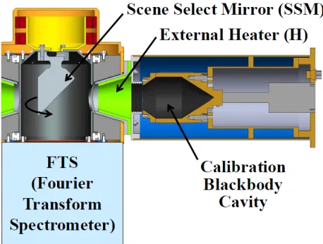
This study focuses on determining which parameters in the spectral radiance equation of the calibration blackbody are critical to the blackbody accuracy. The spectral radiance of the calibration blackbody can be broken down into the radiance emitted by the blackbody and the radiance reflected by the blackbody. The re- flected radiance portion is composed of the all flux en- tering the blackbody from all other surfaces surrounding the blackbody, and reflected back out by the blackbody. For a preliminary study, the surrounding surfaces are categorized as either the blackbody external heater, or the

FTS, which in this case includes all the blackbody

sur-roundings except the heater. The external heater is a de-vice used periodically to measure the blackbody reflec-tance.

The major components of the system are shown in

Figure 1. For this analysis, the scene select mirror (SSM)

and its housing are assumed to be at the same tempera-ture as the FTS, so its effects are lumped together with

the FTS. The SSM is a “barrel-roll” type of mirror that

rotates to allow the FTS to view different radiation

sources, one of which is the calibration blackbody. Equa-tion (1) is the expression for the spectral radiance of the calibration blackbody for this simplified model [7].



















, , ,

, 1

c c c c c c h h h

FTS FTS FTS

L T P T P T F

P T F

     

 



  _



  _ (1)

The Planck radiation equation for spectral radiance at

wavenumber  and temperature T, in units of

W·m–2_·sr–1_·(cm–1₎–1 _is





_

_

_

_

exp 100 1

hc

P T

hc kT

 

  

 (2)

Equation (1) may not be adequate to describe the con-ditions for the on-orbit calibration accuracy required by

Figure 1. FTS, Scene Select Mirror Assembly, and Calibra-tion Blackbody.

the CLARREO IR instrument, in that it does not account for the individual contributions to the reflected radiance by all elements of the blackbody surroundings; rather it lumps them all together into the two terms—heater and

FTS. It is used here as a first order model to allow for a

demonstration of the application of the Design of Ex-periments (DOE) technique to systematically set up an experiment. DOE provides the experimental method (i.e.,

parameter settings and number of runs) to randomly ex- plore all the parameters in Equation (1) without the need to exhaustively examine all of the infinitely possible permutations of parameter values.

Although the system under the study is simple and has been well studied in literature, we would like to empha- size that our intention is to demonstrate the DOE appli- cation with the well-understood system before applying it to the system comprised of the CLARREO IR suite. The total combined uncertainty of the IR Suite will be af-fected by the individual uncertainties of a number of con- tributing components, including for example, the calibra-tion blackbody, the cold scene source, the system non- linearity, and the contributions of several elements of the

FTS, especially the detector and optical systems. There

are a total of 47 parameters that contribute to the total combined uncertainty. Because the CLARREO IR meas- urement accuracy requirement is very stringent, a fol- low-up study has been planned to exhaustively examine as many of the large number of possible permutations of these 47 parameters as possible. The DOE method will provide significant benefit in systematically setting up an experiment to explore the effects of all 47 parameters with an optimal number of runs.

2. Method

A parametric study is usually performed to gain some insight on how changes in parameters affect the changes in the response or output. Traditionally, it changes one parameter at a time (OPAT) while keeping all other rameters at their nominal values, and observes the pa-rameter’s effect on the response. This OPAT method works well if the response behaves the same way when a particular parameter changes, regardless of the values at which all other parameters are set, i.e., main effect.

However, if the responses can behave differently, de-pending on the values of the other parameters, e.g. the cross-term effect, then this OPAT method will fail to capture that dependence.

FTS h T

process can be used to identify critical characteristics that should be designed, manufactured, and/or controlled with special care.

ate the responses. However, because our main objective here is to screen for critical parameters and to understand cross-term effects, we develop a procedure to determine statistically which parameters should be retained in a parsimonious model. Those retained parameters are our critical parameters.

We code Equations (1) and (2) in MATLAB. If we know the values of all parameters on the right hand side of Equation (1), we can then calculate the spectral radi-ance of the calibration blackbody as a function of all wavenumbers. The obtained radiance is treated as truth because all parameters are known without any uncer-tainty associated with them. On the contrary, if all pa-rameter values are assumed to follow a Normal distribu-tion that has the estimated mean and standard deviadistribu-tion, then the obtained radiance distribution will also be Nor-mal, with the estimated mean (i.e., the truth) and

stan-dard deviation (i.e., the total radiance uncertainty). We

would like to get a good estimate of this total radiance uncertainty. In this study, we will use computer simula-tions to estimate the total uncertainty.

The parsimonious model is based on a second-order Taylor series expansion, excluding the pure quadratic terms, as

0 1 2 3 4 5

6 7 8 9 10

11 12 13 14

15 16 17 18

105

...

c

c h

c h FTS

FTS

L c h FTS c

FTS

T T T F

c h c FTS c c c h

T F

U T

T F U U U

U U U U

T T

U U

  

        

    

   

         

 

     

    

   

   

  

(3)

All ’s and their corresponding uncertainties are esti-mated from simulation results. There are 5 versions of this equation, one for each wavenumber. For screening

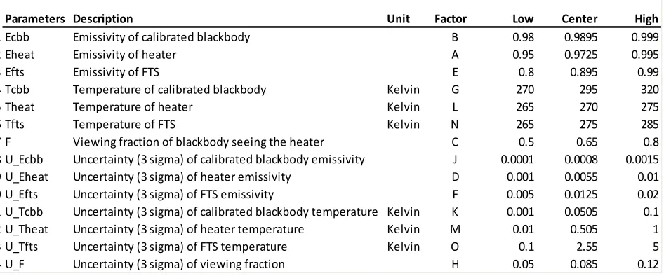
Figure 2 provides details of the experiment chosen for

this study. There are 5 responses, which are uncertainty (1 standard deviation) of the calibration blackbody radi-ance at wavenumbers 200, 600, 1000, 1400, and 2000 cm–1_{. Fourteen input parameters are investigated. The}

first 7 inputs are parameters in Equation (1), while the last 7 inputs are their corresponding uncertainties (at 3 standard deviations). Experimental ranges for all inputs are given as low and high possible values. These ranges are chosen to represent the current known specifications at the time of this study. The center values are the mid-points of the experimental ranges. There would be an infinite number of possible combinations if we were to randomly select input values from these ranges to gener-

purposes, we do not need to know the coefficients of the purely quadratic terms in Equation (3), but rather we need to determine if they should be included in the next sequential experiment. Therefore, there are 106 unknown coefficients (i.e., 1 for the intercept, 14 for the main

in-dependent parameters, and 91 for the cross-term effects). We will need at least 106 unique combinations of all 14 parameters to be able to determine all coefficients.

When selecting these unique parameter combinations, we only need to test the lower and upper values of all parameters. For example, if outputs at low and high val-ues of c are not different significantly, then c is

unlikely to be significant. On the contrary, if both end

Responses Uncertainty (1 sigma) of calibrated blackbody in W m‐2sr‐1(cm‐1)‐1  at wavenumbers 200, 600, 1000, 1400, and 2000 cm‐1

Parameters Description Unit Factor Low Center High

1 Ecbb Emissivity of calibrated blackbody B 0.98 0.9895 0.999

2 Eheat Emissivity of heater A 0.95 0.9725 0.995

3 Efts Emissivity of FTS E 0.8 0.895 0.99

4 Tcbb Temperature of calibrated blackbody Kelvin G 270 295 320

5 Theat Temperature of heater Kelvin L 265 270 275

6 Tfts Temperature of FTS Kelvin N 265 275 285

7 F Viewing fraction of blackbody seeing the heater C 0.5 0.65 0.8

8 U_Ecbb Uncertainty (3 sigma) of calibrated blackbody emissivity  J 0.0001 0.0008 0.0015

9 U_Eheat Uncertainty (3 sigma) of heater emissivity  D 0.001 0.0055 0.01

10 U_Efts Uncertainty (3 sigma) of FTS emissivity  F 0.005 0.0125 0.02

11 U_Tcbb Uncertainty (3 sigma) of calibrated blackbody temperature Kelvin K 0.001 0.0505 0.1

12 U_Theat Uncertainty (3 sigma) of heater temperature Kelvin M 0.01 0.505 1

13 U_Tfts Uncertainty (3 sigma) of FTS temperature Kelvin O 0.1 2.55 5

14 U_F Uncertainty (3 sigma) of viewing fraction H 0.05 0.085 0.12

values have statistically different outputs, then c is

likely to be one of the significant parameters in the first order (linear) sense. To investigate the cross-term effects, for example,  c h, we keep h at its low value and

observe the output gradient of changing c from low to

high, compare this gradient to that of when h at its

high value. If both gradients are not significantly differ-ent, then  c h is unlikely to be significant, and vice

versa. There could be a case where the output may have a concave or convex bell shape, in which the center value has the lowest/highest output. So testing only at the ends is not sufficient if both ends have the same outputs. To guard against this situation, we add a few center runs in which all parameters are set at their center values. If the average center run output is higher than the average out-put at all ends, then we know that the linear model assump-tion is invalid. In that case, we can add sequential runs to determine the purely quadratic or higher-order terms.

In this screening experiment we use a 128th _{fraction of}

the 214 _{factorial design with 10 center points (}

i.e., 214 7IV



+ 10 center points). This is a resolution IV design, in which no main effect is aliased with any other main ef- fect or cross-term effect, but cross-term effects are ali- ased with each other. We may perform a sequential ex- periment if we have to de-alias cross-term effects to ac- curately conclude the results from this screening experi- ment. Empirically, it is less likely that higher-order cross-terms significantly contribute to the response [8]. Therefore, it is unlikely that we will lose any significant information by using this design.

There is a rationale for assigning factor letters to pa-rameters (column “Factor” in Figure 2). We use

sub-ject-matter judgment based on the alias structure of the

design. The more likely parameters can be assigned to factors that alias with the less likely ones. The low con-fidence parameters (or ones with limited knowledge) are assigned to factors that only alias with three-factor or higher-order cross-terms. With this strategy, we feel more confident when drawing conclusions.

The chosen design requires 138 runs. Out of 138 runs, 128 runs are unique parameter combinations of the low and high values, and the other 10 are repeated with all parameters the same, and set at their center values. Since all experiment runs are computer simulations, it may seem that runs using duplicated values would give the same output. However that is not the case, because each time the duplicated values are run, different random numbers are used to estimate the radiance uncertainties.

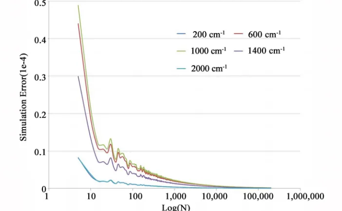
We investigate the quality of computer simulation re-sults. The mean radiance of the simulation solutions has to be an unbiased estimator of its corresponding truth radiance. This mean radiance changes as the number of simulations increases. We evaluate the sensitivity of us-ing different numbers of simulations to simulation error (the uncertainty of the mean). We would expect simula- tion error to improve as the number of simulations in- creases. This technique is referred to as Variance Reduc- tion technique [9]. Simulation error can be calculated from

























1 2

,

1 2

,

Simulation Error ,

, c MC

c MC

Var L T

Var L T N



 



(4)

Figure 3 shows the sensitivity of the number of

simu-lations to the simulation error for a randomly selected run

from our 138 runs. The error converges to the minimum value after 10,000 simulations. For our study, we can therefore use 10,000 simulations for each of 138 runs. However, a general practice often suggests 100,000 si- mulations to guarantee convergence to the minimum un- certainty of the mean. We therefore choose N to be 100,000 for our study.

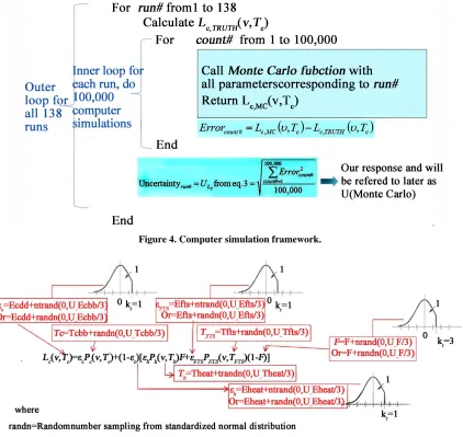
Figure 4 shows the detail on how the computer

simu-lation is done. The outer loop is repeated 138 times, one for each run. We produce a 100,000 by 5 array of cali-bration blackbody radiances for each run. Row represents 100,000 different sets of random numbers used in the simulation. Column represents 5 different wavenumbers of interest. Also produced for each run is the truth radi-ances (a 1 by 5 array) when all parameters do not have any uncertainty. Uncertainty for each run is then esti-mated based on root mean squared error.

Details of Monte Carlo function are given in Figure 5.

The temperature of the calibration blackbody is assumed to follow a Normal distribution with its mean and stan-dard deviation given by Tcbb and U_Tcbb/3, respec-tively. Similar distribution assumptions apply for tem-peratures of the heater and the FTS. Due to the physical

limit of emissivities and view factors (i.e., must be less

than or equal to 1), their distributions are handled differ-ently than those of temperatures. For any runs with low Ecbb value (0.98), the emissivity of the calibration blackbody is assumed to follow a Normal distribution with mean and standard deviation given by Ecbb (0.98) and U_Ecbb/3 (0.0001/3), respectively. This is because it is unlikely for these runs to have any Ecbb’s sampled from this distribution greater than 1. We have validated this during our experiment. Similar Normal distribution assumptions apply for emissivities of the heater and the

FTS, and the view factor of any runs with low values. On

the other hand, for any runs with high Ecbb value (0.999),

Figure 4. Computer simulation framework.

its distribution is assumed to follow Right Truncated Normal (RTN) distribution. This RTN distribution can be thought of as the right-bounded Normal distribution, where the sampled Ecbb values cannot exceed 0.9995 (or Ecbb + kr × U_Ecbb/3 = 0.999 + 1 × 0.0015/3). RTN

distributions are also assumed for emissivities of heater and FTS, and view factor of any runs with high values.

The sampled Eheat, Efts, and F values are not allowed to

exceed 0.9983, 0.9967, and 0.92, respectively. The right- bounded values (kr) are subjectively chosen and should

not have an impact on the findings of the screening ex-periment as long as the sample values do not exceed 1.

When running this experiment, we partition our 138 runs into 2 blocks of 69 each. This is done to ensure that the actual batch execution on a personal computer for each block can be complete without interruption, such as power shutdown, or any other computer related issues. We also randomize all runs to guard against possible unknown bias (e.g., random number quality) that could sabotage our findings. Our design is in fact a randomized complete block experiment [8].

3. Results

We used Minitab [10] in setting and analyzing this ex-periment. The factorial experiment is usually analyzed by using Analysis-of-Variance (ANOVA). We investigated to make certain that none of ANOVA assumptions (nor-mality, independency, and constant variance of residuals) is violated. There is no strong evidence of any violations. Block effect has no statistical effect on the responses. In

other words, our responses do not depend on when the computer simulation is run. This also implies that the quality of random numbers is good. Figure 6

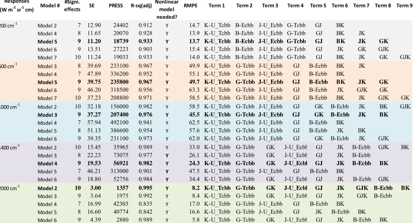
summa-rizes the analysis. For each wavenumber, we test several models (in the form of Equation (3)) with different num- ber of significant regression coefficients based on ANOVA and 95% confidence level. These are reported in column “#Signi. Effects”, which includes the intercept term. The last 9 columns provide the significant terms in descend- ing order of the coefficient magnitudes for all models under investigation.

Standard error (SE), prediction error sum of squares (PRESS), and total variation explained by the model, adjusted for appropriate number of terms in the model (R-sq(adj)) are statistics measures to determine the best model. They are reported in columns “SE”, “PRESS”, and “R-sq(adj)”, respectively. The “Quadratic/Nonlinear model needed?” column indicates if the model requires pure quadratic terms and higher-order terms. These are to test the hypothesis of whether or not the center-point average differs from the average at all ends. All models suggest that they are. Therefore, we will need to add ad-ditional runs if we were to use the model to predict the calibration blackbody uncertainty more accurately.

We also perform an additional 138 confirmation runs to check model predictability. These confirmation runs are another 128th _{fraction of the 2}14 _{factorial design with}

10 center points. Column “RMPE” (root mean square prediction error) shows how well each model predicts based on these 138 confirmation runs. The RMPE is cal-culated from

Responses        (W m‐2

 sr‐1 cm) Model # #Signi. 

effects SE PRESS R‐sq(adj)

Quadratic/ Nonlinear  model  needed?

RMPE Term 1 Term 2 Term 3 Term 4 Term 5 Term 6 Term 7 Term 8 Term 9

200 cm‐1 _{Model 2 7 12.90 24402 0.912 Y 14.7 K-U_Tcbb B-Ecbb J-U_Ecbb G-Tcbb GJ BK}

Model 4 8 11.65 20070 0.928 Y 13.9 K-U_Tcbb B-Ecbb J-U_Ecbb G-Tcbb GJ BK JK

Model 5 9 11.20 18739 0.933 Y 13.7 K-U_Tcbb B-Ecbb J-U_Ecbb G-Tcbb GJ BK JK GK

Model 6 9 13.51 27223 0.903 Y 15.4 K-U_Tcbb B-Ecbb J-U_Ecbb G-Tcbb GJ JK GK GJK

Model 7 10 11.24 19033 0.933 Y 14.0 K-U_Tcbb B-Ecbb J-U_Ecbb G-Tcbb GJ BK JK GK GJK

600 cm‐1 _{Model 3 8 39.69 233100 0.967 Y 49.9 K-U_Tcbb G-Tcbb J-U_Ecbb GJ B-Ecbb BK JK}

Model 4 7 47.89 336200 0.952 Y 55.1 K-U_Tcbb G-Tcbb J-U_Ecbb GJ B-Ecbb BK

Model 5 9 39.75 235800 0.967 Y 49.7 K-U_Tcbb G-Tcbb J-U_Ecbb GJ B-Ecbb BK JK GK

Model 6 9 46.20 318500 0.956 Y 63.3 K-U_Tcbb G-Tcbb J-U_Ecbb GJ B-Ecbb JK GJK GK

Model 7 10 37.23 208800 0.971 Y 58.5 K-U_Tcbb G-Tcbb J-U_Ecbb GJ B-Ecbb BK JK GJK GK

1000 cm‐1 _{Model 2 10 32.18 156000 0.982 Y 58.5 K-U_Tcbb G-Tcbb J-U_Ecbb GJ GK B-Ecbb JK BK GJK}

Model 3 9 37.27 207400 0.976 Y 45.5 K-U_Tcbb G-Tcbb J-U_Ecbb GJ GK B-Ecbb JK BK

Model 4 7 57.94 492100 0.941 Y 62.5 K-U_Tcbb G-Tcbb J-U_Ecbb GJ B-Ecbb BK

Model 5 8 51.13 386600 0.954 Y 57.6 K-U_Tcbb G-Tcbb J-U_Ecbb GJ B-Ecbb JK BK

Model 6 9 39.35 231100 0.973 Y 62.0 K-U_Tcbb G-Tcbb J-U_Ecbb GJ GK B-Ecbb JK GJK

1400 cm‐1 _{Model 2 10 15.45 35965 0.989 Y 33.0 K-U_Tcbb G-Tcbb GK J-U_Ecbb GJ JK B-Ecbb GJK BK}

Model 3 8 22.23 73075 0.977 Y 26.1 K-U_Tcbb G-Tcbb GK J-U_Ecbb GJ JK B-Ecbb

Model 4 9 19.53 56921 0.982 Y 24.3 K-U_Tcbb G-Tcbb GK J-U_Ecbb GJ JK B-Ecbb BK

Model 5 7 46.21 313000 0.901 Y 47.5 K-U_Tcbb G-Tcbb J-U_Ecbb GJ B-Ecbb BK

Model 6 9 18.80 52756 0.984 Y 34.4 K-U_Tcbb G-Tcbb GK J-U_Ecbb GJ JK B-Ecbb GJK

2000 cm‐1 _{Model 2 10 3.00 1357 0.995 Y 8.2 K-U_Tcbb G-Tcbb GK J-U_Ecbb GJ JK GJK B-Ecbb BK}

Model 3 9 3.64 1975 0.992 Y 8.4 K-U_Tcbb G-Tcbb GK J-U_Ecbb GJ JK GJK B-Ecbb

Model 4 7 16.99 42303 0.835 Y 17.0 K-U_Tcbb G-Tcbb J-U_Ecbb GJ B-Ecbb BK

Model 5 8 16.60 40774 0.842 Y 16.6 K-U_Tcbb G-Tcbb J-U_Ecbb GJ JK B-Ecbb BK

Model 6 9 4.39 2880 0.989 Y 5.8 K-U_Tcbb G-Tcbb GK J-U_Ecbb GJ JK B-Ecbb BK

B = Ecbb; G = Tcbb; J = U_Ecbb; K = U_Tcbb; BK= Ecbb*U_Tcbb; GK = Tcbb*U_Tcbb; GJ = Tcbb*U_Ecbb; JK = U_Ecbb*U_Tcbb; GJK = Tcbb*U_Ecbb*U_Tcbb.









1

ˆ

RMPE n Monte Carlo _i i

i

U U







Note that PRESS and RMPE are quite similar. How-ever, the PRESS is based on the data that is used to fit the model, while the RMPE is based on the new data that are not used during model fitting. More coefficient terms in the model usually improve PRESS, but may result in poor RMPE. This is the case when we over-fit the model (see an example in Figure 6, for 1000 wavenumber,

Models 2 and 3).

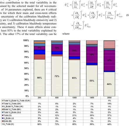
The best model can be determined based on the mini-mum SE, PRESS, R-sq(adj), and RMPE statistics. By subjectively evaluating using these four statistics, the best model for each wavenumber was selected (bold font in Figure 6). Figure 7 provides critical parameters and

their relative contribution to the total variability in the data explained by the selected model for all wavenum-bers. Out of 14 parameters explored, there are 4 critical parameters for which their main and cross-term effects drive the uncertainty of the calibration blackbody radi-ance. They are 1) calibration blackbody emissivity and 2) its uncertainty, and 3) calibration blackbody temperature and 4) its uncertainty. These 4 main effects alone con- tribute at least 83% to the total variability explained by the model. The other 17% of the total variability can be

explained by their cross-term effects. Deending on wave- numbers, each effect contributes differently to the total variability. For example, at 200 wavenumber, the highest two contributors are U_Tcbb and Ecbb, while at other wavenumbers, the highest two are U_Tcbb and Tcbb. We also observe that at 2000 wavenumber, a three-factor cross-term, Tcbb*U_Tcbb* U_Ecbb, is significant, while this cross-term is not significant at other wavenumbers.

Up to this point, we have used computer simulation to estimate uncertainty of the calibration blackbody radi-ance. We can also use the propagation of uncertainty law as described in Taylor and Kuyatt [11], Gertsbakh [12], and Coleman and Steele [13] to calculate uncertainty. Applying the propagation of uncertainty to Equation (1), assuming that all cross terms are negligible, gives

2 2 2

2 2 2 2

2 2 2

2 2

2 2

c c c

h F

FTS

c c c

L P

c c h

c c c

P F

h F

c P FTS

L L L

U U U U

P

L L L

U U

P F

L U P

 



 



     

_  _  _ 

     

      

_{ } _{ } _{ }

 _ _ 

   

    _ 

 

2 h

TS TS

U (6)

where





c h h FTS FTS

c L

P  P F  P F

       c c h h L P F     





 





c FTS

FTS L

F

P  



 







c

c h h FTS FTS

L

P P

F   



 







2 , 2

c c c P T c P T U U T     _ _   





2 , 2

h h h P T h P T U U T     _ _   





2 , 2

FTS FTS FTS P T FTS P T U U T     _ _   

The quality of uncertainty estimates from Equation (6) depends on the validity of the assumption that the uncer-tainty contributors are independent (i.e., the cross terms

are insignificant). On the other hand, the quality of un-certainty estimates from simulation depends on the qual-ity of random numbers and sufficient number of simula-tion runs, which has been demonstrated earlier to have good quality.

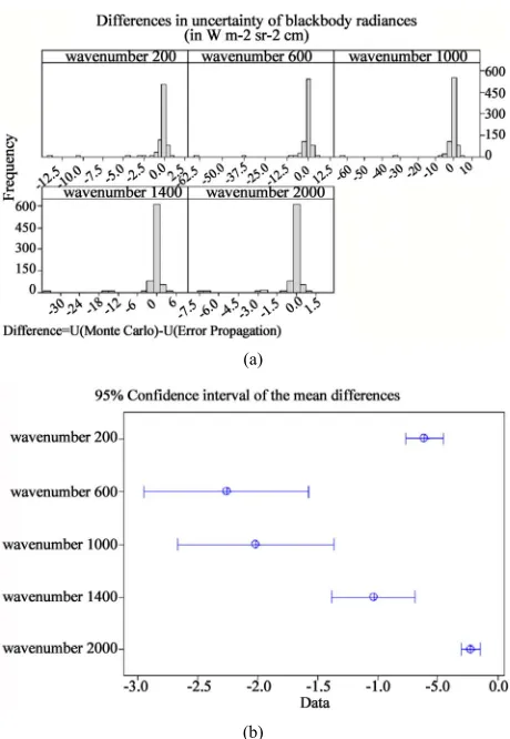
We estimate the uncertainties of the calibration black-body using Equation (6) with the same parameter settings as in those from 138 simulated experimental runs, and from 138 simulated confirmation runs. We also include additional 523 experimental runs for the same parameter ranges to explore uncertainties obtained from the 2 methods. Figure 8(a) provides histograms of 799 (138 +

138 + 523) differences in uncertainty between the two approaches. Specifically,







DifferenceU Monte Carlo U Error Propagation



(7) Based on our observation, the differences have high tendency to be zero, but they may not follow a Normal distribution because of the very long tail on the left. Re-gardless of the distributions of the differences, the mean

(a)

(b)

(a) Histograms of differences in uncertainty of blackbody radiances. (b) 95% Confidence interval of the mean differences in uncertainty of black-body radiances.

Figure 8. Analysis of differences in uncertainty of black-body radiances obtained by simulation and Uncertainty Propagation methods.

differences will follow the Normal distribution according to the Central Limit Theorem. Figure 8(b) shows the

95% confidence intervals of the mean differences. All intervals do not cover zero. Therefore, on average the computer simulation and the propagation of uncertainty methods produce different uncertainties in the calibration blackbody radiances for all wavenumbers. Because the mean differences are negative, on average the propaga-tion of uncertainty method estimates higher uncertainties than those from the computer simulation approach. We suspect that the cross terms excluded in Equation (6) must be negative on average.

We observe from our data (not shown) that radiance uncertainties vary depending on wavenumbers, regard-less which method is used. Uncertainties are smaller for wavenumbers 200 and 2000 cm–1_{, because their}

radi-ances are smaller. In Figure 8(b), the interval widths of

the mean differences vary depending on wavenumbers, with tighter widths for wavenumbers 200 and 2000 cm–1_.

predictable than those of other wavenumbers. Rather their tighter widths may in fact be proportional to the magnitudes of the absolute radiances. Therefore, we normalize all differences by their associated relative un-certainty from simulation (Unun-certainty Difference/U (Monte Carlo). Figure 9 shows similar analyses as in Figure 8, but for normalized differences.

The normalized differences (in %) have a high ten-dency to be zero. On average, the normalized differences are not zero, but are negative. In the worst case across all 5 wavenumbers, the mean normalized differences can be as high as –1.2%. On average, the cross terms in the propagation of uncertainty method must be negative. The interval widths of the mean normalized differences are now consistent across wavenumbers.

4. Conclusions and Future Works

The on-orbit blackbody calibration source of the CLAR-REO IR Suite is one of the most critical components in obtaining accurate CLARREO IR measurements. To

(a)

(b)

(a) Histograms of normalized differences. (b) 95% Confidence interval of the mean normalized differences (%).

Figure 9. Analysis of normalized differences in uncertainty of blackbody radiances obtained by simulation and Uncer-tainty Propagation methods.

achieve such accuracy, CLARREO relies on highly ac-curate knowledge of the spectral radiance of the calibra-tion blackbody. This study focuses on determining which parameters in the spectral radiance equation of the cali-bration blackbody are critical to the blackbody accuracy. Based on the spectral radiance equation used in this study, fourteen parameters were identified and explored. The Design of Experiments (DOE) method was applied to systematically set up an experiment to provide parameter settings and number of runs in order to explore these 14 parameters. The experiment was done by computer simulation to estimate the total radiance uncertainty. The sensitivity of number of simulations to simulation error was explored and used to determine the number of simu-lations.

All explored parameters’ ranges were based on the current known specifications available at time of this study. A 128th _{fraction of the 2}14 _{factorial design with 10}

center points (i.e., 214 7IV

 _{+ 10 center points) was chosen}

for this study. It is a resolution IV design, in which no main effect is aliased with any other main effect or cross-term effect, but cross-term effects are aliased with each other. This design was sufficient for the screening purpose to determine which of these parameters were critical to the total radiance uncertainty of the calibration blackbody. The parsimonious models based on a sec-ond-order Taylor series expansion were fit based on the experimental uncertainty data. Another 128th _{fraction of}

the 214 _{factorial design with 10 center points were run}

and used as confirmation points to check the models for predictability. The best models were then chosen based on best statistics of fitting and predicting errors.

Within the explored ranges, only 4 out of 14 parame-ters were discovered to be critical and should be designed, manufactured, and controlled carefully. They were emis-sivity of blackbody, temperature of blackbody, uncer-tainty of blackbody emissivity, and unceruncer-tainty of black-body temperature. Emissivities and temperatures, and their associated uncertainties, for other surfaces sur-rounding the blackbody were less critical to the total blackbody uncertainty. The uncertainties obtained by simulation were also compared to those from the propa-gation of error method. The two methods produced sta-tistically different uncertainties and the differences were suspected to be due to the first-order assumption in the propagation of uncertainty. Nevertheless, the differences were small and were considered to be not practically dif-ferent.

indi-vidual uncertainties of a number of contributing compo-nents. There are a total of 47 parameters that contribute to the total combined uncertainty. Because the CLAR-REO IR measurement accuracy requirement is very stringent, a follow-up study has been planned to apply the DOE in systematically setting up an experiment to explore the effects of all 47 parameters. It is our believe that the DOE method will help identifying critical pa-rameters to the total IR measurement uncertainty that need to be effectively and efficiently designed to meet the instrument accuracy requirement within the limited resources.

5. Acknowledgements

We would like to thank Dave G. Johnson and Alan D. Little at NASA Langley Research Center for their valu-able perspectives for this work.

REFERENCES

[1] J. A. Anderson, et al., “Decadal Survey Clarreo Mission,”

Clarreo Workshop, Adelphi, 2007.

http://map.nasa.gov/documents/CLARREO/7_07_present ations/JAnderson_071707.pdf

[2] Clarreo Team, “Clarreo Mission Overview,” NASA Langley Research Center, Hampton, 2011.

http://clarreo.larc.nasa.gov/docs/CLARREO_Mission_Ov erview_Jan%202011.pdf

[3] G. Ohring, “Achieving Satellite Instrument Calibration for Climate Change,” US Department of Commerce, 2008.

[4] National Research Council, “Earth Science and Applica-tions from Space: National Imperatives for the Next Decade and Beyond,” National Academies Press, 2007. http://www.nap.edu/catalog.php?record_id=11820

[5] J. A. Dykema and J. G. Anderson, “A Methodology for Obtaining On-Orbit SI-Traceable Spectral Radiance Mea- surements in the Thermal Infrared,” Metrologia, Vol. 43,

No. 3, 2006, pp. 287-293.

doi:10.1088/0026-1394/43/3/011

[6] F. A. Best, D. P. Adler, C. Pettersen, H. E. Revercomb, P. J. Gero, J. K. Taylor and R. O. Knuteson, “On-Orbit Ab-solute Radiance Standard for Future IR Remote Sensing Instruments,” The 2011 Earth Science Technology Forum,

Pasadena, 2011.

http://estohttp://esto.nasa.gov/conferences/estf2011/paper s/Best_ESTF2011.pdf

[7] P. J. Gero, J. A. Dykema and J. G. Anderson, “A Black- body Design for SI-Traceable Radiometry for Earth Ob- servation,” Journal of Atmospheric and Oceanic Tech- nology, Vol. 25, No. 11, 2008, pp. 2046-2054.

doi:10.1175/2008JTECHA1100.1

[8] D. C. Montgomery, “Design Analysis of Experiments,” 7th Edition,John Wiley & Sons, Inc.,Hoboken, 2009. [9] S. M. Ross, “Simulation,” 4th Edition, Elsevier, Inc.,

Houston, 2006.

[10] Minitab Version 15.1.30.0., Minitab, Inc., State College, 2007.

[11] B. N. Taylor and C. E. Kuyatt, “Guidelines for Evaluating and Expressing the Uncertainty of NIST Measurement Results,” NIST Technical Note, Vol. 1297, 1994.

[12] I. Gertsbakh, “Measurement Theory for Engineers,” Springer, Berlin, 2003.

[13] H. W. Coleman and W. G. Steele, “Experimentation, Validation, and Uncertainty Analysis for Engineers,” 3rd Edition, John Wiley & Sons, Inc., Hoboken, 2009.

doi:10.1002/9780470485682

[14] M. P. Taylor and D. B. Newell, “CODATA Recommend- ed Values of the Fundamental Physical Constants: 2006,”

Reviews of Modern Physics, Vol. 80, No. 2, 2008, pp.

Nomenclature



 Wavenumbers: 200, 600, 1000, 1400, and 2000 cm−1 

h Planck Constant = 6.62606896 × 10−34 Js [14] 

c Speed of light in a vacuum = 2.99792458 × 108 m/s

[14]



k Boltzmann constant = 1.3806504 × 10−23 JK−1 [14] 

c T

 T

Temperature of calibration blackbody (K)

h  T

Temperature of heater (K)

FTS , ( T L 

Temperature of FTS (K) 

) c

c Radiance of calibration blackbody as a function

of wavenumber and its temperature (W·m−2_·sr−1_·(cm−1₎−1₎ 

) , ( _c c T

P  Radiance calculated from Planck’s equation

for calibration blackbody as a function of wavenumber and its temperature (W·m−2_·sr−1_·(cm−1₎−1₎



) , ( _h h T

P  Radiance calculated from Planck’s equation

for heater as a function of wavenumber and its tempera-ture (W·m−2_·sr−1_·(cm−1₎−1₎



) , ( _FTS FTS T

P  Radiance calculated from Planck’s

equa-tion for FTS as a function of wavenumber and its

tem-perature (W·m−2_·sr−1_·(cm−1₎−1₎ 

c

 Emissivity of calibration blackbody

 h

 Emissivity of heater

 FTS

 Emissivity of FTS



F View factor of the heater, as seen from the

black-body aperture

 c

 Reflectance of calibration blackbody (_c 1_c)

 c L

U Uncertainty in the calibration blackbody radiance

(W·m−2_·sr−1_·(cm−1₎−1₎ 

c

U_ Uncertainty in the calibration blackbody emissivity 

c P

U Uncertainty in the calibration blackbody Planck

radiance, which is a function of blackbody temperature (W·m−2_·sr−1_·(cm−1₎−1₎

 h

U_ Uncertainty in the heater emissivity 

h P

U Uncertainty in the heater Planck radiance, which is

a function of heater temperature (W·m−2_·sr−1_·(cm−1₎−1₎ 

F

U Uncertainty in the view factor of the heater, as seen

from the blackbody aperture

 FTS

U_ uncertainty in the FTS emissivity 

FTS P

U Uncertainty in the FTS Planck radiance, which is

a function of FTS temperature (W·m−2·sr−1·(cm−1)−1) 

c T

U Uncertainty in the calibration blackbody

tempera-ture (K)

 h T

U Uncertainty in the heater temperature (K) 

FTS T

U Uncertainty in the FTS temperature (K) 

s '

 The regression coefficients which are estimated

from computer simulated experiment



 The random fitting error



) , (

,MC c

c T

L  Spectral radiance of calibration blackbody

obtained from simulation as a function of wavenumber and its temperature (W·m−2_·sr−1_·(cm−1₎−1₎



) , (

,MC c

c T

L  Mean radiance of the calibration

black-body obtained from simulation as a function of wave-number and its temperature (W·m−2_·sr−1_·(cm−1₎−1₎



N Number of simulation runs



n Number of confirmation runs 

i

U(MonteCarlo) Uncertainty obtained from Monte

Carlo function for ith confirmation run 

i

Uˆ Predicted uncertainty obtained from the model for