http://www.scirp.org/journal/jgis ISSN Online: 2151-1969
ISSN Print: 2151-1950
DOI: 10.4236/jgis.2018.101003 Feb. 2, 2018 57 Journal of Geographic Information System
Application of Remote Sensing Techniques and
Geographic Information Systems to Analyze
Land Surface Temperature in Response to Land
Use/Land Cover Change in Greater Cairo Region,
Egypt
Mohamed Aboelnour
1,2, Bernard A. Engel
1*1Department of Agriculture and Biological Engineering, College of Engineering, Purdue University, West Lafayette, IN, USA
2Geology Department, Faculty of Science, Suez Canal University, Ismailia, Egypt
Email: [email protected], *[email protected]
Abstract
The Greater Cairo Region (GCR), Egypt has experienced rapid urban expan-sion and broad development over the past several decades. Due to such de-velopment, this region faces many environmental consequences. In order to mitigate such consequences, it is essential to examine the historical change to measure the urban sprawl of GCR, and its effect on land surface temperature (LST). The objective of this study is to fulfill this goal. It does so by generating land use/land cover (LULC) maps derived from Landsat 5 TM for 1990 and 2003 and Landsat 8 OLI for 2016, using several classification techniques. A spectral radiance model and a web-based atmospheric correction model were used to successfully evaluate LST from thermal bands of Landsat data. Overall accuracy of Landsat derived land use data were 90.3%, 96.5% and 94.9% for years 1990, 2003 and 2016, respectively. The LULC change analysis revealed vegetation loss to urban land by an amount of 7.73% and from barren lands to urban uses by 8.70% within a 26-year timespan (1990-2016). This rapid urban growth significantly decreases vegetation areas, consequently increasing the LST and modifying the urban microclimate. Results from this study can help policy-makers characterize the evolution of urban construction for future de-velopments.
Keywords
Landsat, Land Surface Temperature, Land Use Change, Accuracy Assessment, Greater Cairo Region
How to cite this paper: Aboelnour, M. and Engel, B.A. (2018) Application of Remote Sensing Techniques and Geographic Infor- mation Systems to Analyze Land Surface Temperature in Response to Land Use/Land Cover Change in Greater Cairo Region, Egypt. Journal of Geographic Information System, 10, 57-88.
https://doi.org/10.4236/jgis.2018.101003
Received: December 7, 2017 Accepted: January 30, 2018 Published: February 2, 2018
Copyright © 2018 by authors and Scientific Research Publishing Inc. This work is licensed under the Creative Commons Attribution International License (CC BY 4.0).
DOI: 10.4236/jgis.2018.101003 58 Journal of Geographic Information System
1. Introduction
Cities are dynamic due to unavoidable changes that can be assigned to many factors. One of the main factors behind these changes is urban growth and pop-ulation expansion [1]. As the population of a given area increases, the interest for new settlements continues increasing at the expense of other land cover classes, for instance, vegetation and barren lands. Land surface impacts that oc-cur during the process of urbanization include, but are not limited to, soil com-paction, vegetation reduction and change from permeable to impervious surfac-es as buildings, parking lots and roads are constructed. A seeming lack of plan-ning of land use/land cover (LULC) has been a problem at a local and regional scale, making it a major issue in the study of worldwide ecological change [2] [3] [4]. Such changes have many implications for human society, environmental re-silience, and water issues, such as the alteration of runoff, infiltration and groundwater discharge [5]. In addition, poor water quality occurs due to a lack of planning with comprehensive arrangements or any consideration regarding their effects on nature. Nevertheless, an increase in land surface temperatures (LST) is one of the key effects of LULC changes [6]-[11]. Increases in LST over the past several decades are considered a major issue in urban regions, due to the conversion of vegetation cover to impervious cover [12], which in turn has a negative impact on people [13], affects many environmental processes and mod-ifies the degree of solar radiation’s absorption, evaporation rates, desertification, air pollution, albedo, heat storage, wind turbulence and many aspects of the wa-ter balance [14]. Therefore, the impact on environmental processes cannot be well-understood and mitigated without understanding the impacts of climate change, the interaction between the earth and the atmosphere and knowledge of land use/land cover change at various scales that drive them [2].
Using remote sensing data in conjunction with Geographic Information Sys-tems (GIS) proved effective for mapping urban areas, modeling urban growth and monitoring the dynamic changes of LULC [15] [16]. Remote sensing (RS) provides medium and high spatial, spectral and temporal resolution data with consistent and repetitive coverage of the earth’s surface [17], and a high capabil-ity to extract change information from satellite data [12]. However, LULC change and LST can be monitored by traditional surveys and land based obser-vation stations, as well as satellite data, because it is a time and cost-effective technique that can provide more information with respect to land use’s geo-graphical distribution [7]. Satellite RS techniques, therefore, have become preva-lent in monitoring change detection in both rural and urban regions [18] [19] [20] [21]. As a result, they have been widely used to evaluate LULC change with useful outputs and different scales [22] [23].
DOI: 10.4236/jgis.2018.101003 59 Journal of Geographic Information System
Mapper (TM), Enhanced Thematic Mapper (ETM+) and Operational Land Manger (OLM). Landsat datasets have provided high resolution visible and infrared data, with thermal data and a panchromatic image. In addition, it sup-plies an extraordinary level of information on the classification of several earth components at large scale [24] [25] using a variety of automated change detec-tion techniques and commonly applied classificadetec-tion algorithms (i.e. principle component analysis (PCA), unsupervised clustering, Hybrid, Fuzzy, Bayes and supervised classification). These change detection and classification techniques require personal experience and additional ancillary data with respect to study areas, i.e. a very high resolution aerial images and ground data, which can be used to construct a trustworthy dataset for different classification algorithms that can be used further in training samples and accuracy assessments [7]. Al-though ground data are considered to be the most reliable reference data, such data are often either not accessible or very costly. Therefore, a pre-defined statis-tical characterizations file for the image is created to store a per-pixel signature of a certain land cover class. This uses the stored information and the raw digital number (DN) of each individual pixel in the scene and converts them to ra-diance values. Several researchers and scholars applied similar techniques to achieve satisfactory results. For example, Landsat satellite images themselves were used to evaluate the performance of classification algorithms used to map forest clear cuts in the Pacific Northwest [26]. In addition, supervised classifica-tion maximum likelihood algorithms were applied to detect land cover change in a watershed in Pakistan and India with 95% and 92% overall accuracy, respec-tively [27] [28]. Although a high accuracy is obtained from these results, the presence of other reference data are essential to evaluate the overall accuracy and performance of the created geospatial maps [7].
DOI: 10.4236/jgis.2018.101003 60 Journal of Geographic Information System
of LULC change were identified in some studies, followed by an investigation for the impact of these changes on LST [6] [34].
Cities located in semi-arid and arid regions require more attention to be better evaluated and understood [35]. In many developing countries of the world, in-cluding Egypt, there are limited regional figures on land expense for monitoring urban expansion. Studies revealed that settlements in developing countries grow five times as fast as those in developed ones [15]. The present study focuses mainly on change detection evaluation of LULC and LST in the Greater Cairo Region (GCR) of Egypt for the past several decades, from 1990 to 2016. The GCR contains the largest portion of facilities and services, enabling the founda-tion of dwelling places for qualified work forces that are generally found close to and within the city [36]. Moreover, due to the suitable topographic and geologic setting, the areas surrounding GCR showed the highest proportion of urban ex-pansion. This has contributed to the high rate of population growth, city expan-sion and extravagant development.
The main thrust of this paper is to analyze LULC change through classifica-tions and post-classification change detection techniques by utilizing multi- spectral Landsat TM and OLI data of GCR for 1990, 2003 and 2016 through the integration of remote sensing and GIS. In addition, the use of these Landsat data to estimate LST in GCR will be evaluated through different models and algo-rithms, as described in detail in the methodology section. The current study aims to: 1) quantitatively delineate different LULC classes and evaluate the pat-tern of LULC change from 1990 to 2016 in GCR; 2) provide tools to reliably in-vestigate the variation of LST values in relation to LULC change through time; 3) further evaluate the effect of vegetation on LST as derived from different algo-rithms for satellite imagery through an examination of the NDVI-LST and (Nor- malized Different Built-up Index) NDBI-LST correlation based on statistical analysis methods and the texture of LULC changes, to determine the main caus-es of thcaus-ese environmental changcaus-es; and 4) examine the potential and the accura-cy of RS and GIS utilization in monitoring the spatial distribution of LULC changes. The information gleaned from the validated change detection outputs can help in understanding the dynamics of LULC change in order to help policy- makers predict and plan for future developments in GCR, achieve long-term sustainability of soil and water resources, address impacts of climate change, and therefore characterize the evolution of new hot spots for urban construction lands and infrastructure development.
Two of the most important underlying premises of the objectives tested in the investigation is the opportunity of obtaining a LULC and LST maps from synop-tic view of Landsat images over large spatial areas; and improve thermal studies in Egypt that will be used to justify subsides for law seeking to reduce impacts on thermal comfort in exciting urban areas.
2. Study Area
DOI: 10.4236/jgis.2018.101003 61 Journal of Geographic Information System
Egypt, which includes three sectors. The main sector is the metropolitan Cairo city on the eastern bank of the Nile River, parts of Giza City on the eastern bank of the Nile, and Qalyoubia, north of Cairo. The study area is located at 30˚00'N and 31˚20'E, in the middle and southern part, i.e. apex, of the Nile Delta Region, covering an area of 845,137 hectares (Figure 1). The Nile forms the admistrative division between Cairo and Giza sectors, running through the study area in a floodplain 9 to 35 km wide. This is constricted by hills on both the eastern and western sides, with desert areas extending in the eastern and western direction
[37], characterizing it as a subtropical climatic region with high temperatures and solar radiation, dry and rainless summers, and cold, moist and rainy win-ters [38].
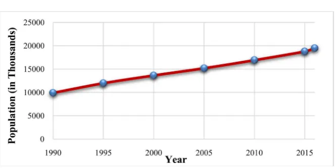
The GCR was selected because of its unique location and climatic conditions, with a diversity of historical heritages, making it one of the most dynamic urban regions in Egypt. It now represents about 23% of the total population of Egypt and 43% of the urban population. While the population expansion has grown tenfold in the whole country, the GCR has grown more than thirty fold in the last century and a half [39]. Half of this expansion has taken place on vegetated and rich agriculture land, while the other half occurs on the agglomeration fringes located at the borders of GCR. Little sporadic growth in the form of new communities has been created on what was desert land on the eastern district. Based on Central Agency for Public Mobilization and Statistics (CAPMAS) es-timation, it appears that GCR has a population of about 20 million as of 2016
[40] (Figure 2).
3. Data Used
3.1. Satellite Data
Landsat 5 TM for 1990 and 2003 and Landsat 8 OLI 2016 were selected due to
[image:5.595.124.540.489.694.2](a) (b)
DOI: 10.4236/jgis.2018.101003 62 Journal of Geographic Information System
Figure 2. Growth of GCR urban population during 1990-2016 according to Central Agen-cy of Public Mobilization and Statistics (CAPMAS) [40].
Table 1. Specification of Landsat satellite images. (*TIR = 120 × 30, data is acquired at 100 m and resampled to 30 m.)
Satellite Sensor Acquisition date Path/Row Number of bands radiometric resolution resolution (m) Spatial
Landsat 5 TM Aug. 4th 1990 176/39 7 8 bit 30 *TIR = 120 × 30
Landsat 5 TM Aug. 8th 2003 176/39 7 8 bit 30 TIR = 120 × 30
Landsat 8 OLI/TIRS Aug. 11th 2016 176/39 11 16 bit 30 TIR = 100 × 30
their high spatial resolution for both multispectral and thermal bands, which benefits an accurate location of different land uses and monitoring LST. Due to their availability, three cloud-free Landsat images were selected to detect changes in the study area: August 4, 1990; August 8, 2003; and August 11, 2016 with scenes along the same path. The details of the Landsat data used in the current study are furnished in Table 1. All the satellite images were acquired during the summer season, intermediate to the agricultural growth season, in which most agricultural fields are green and active, which maximizes the spec-tral difference between these agricultural fields, urban areas and barren lands
[7]. High-quality Landsat data acquisition is available from private and public sources.
3.2. Auxiliary Data
[image:6.595.209.537.301.408.2]DOI: 10.4236/jgis.2018.101003 63 Journal of Geographic Information System
Model (DEM) [41] and road networks [42]. Grouping of different spectral classes was done on the basis of land-cover types obtained from FAO-Land Cover Classification System (LCCS) of 2004, knowledge-based approaches and in-corporated information from organizations and institutions of the Egyptian Governments. The ground truth data were in the form of reference data points used for assessing accuracy of the classification that were selected using high resolution GeoEye and QuickBird imagery [43] in addition to points collected during a field survey using Global Positioning System (GPS) receivers.
Image processing, such as image extraction, rectification, atmospheric correc-tion for Landsat data, restoracorrec-tion and classificacorrec-tion, and GIS analysis and inter-pretation were performed using a set of software to assure higher accuracy: Earth Resources Data Analysis Systems (ERDAS) Imagine 2014, the Environment for Visualizing Images (ENVI 5.3), the Integrated Land and Water Information System (ILWIS), ArcGIS 10.4 (ESRI) software, Python and Statistical Analysis System (SAS) software.
4. Methodology
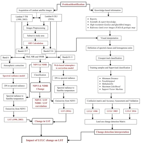
The analysis includes image preprocessing, image classification, land cover in-dices (NDVI and NDBI) derivation and the evaluation of LST using thermal bands in the Landsat dataset. A flowchart of the research process is described and summarized in Figure 3.
4.1. Image Preprocessing
Both Landsat TM and OLI data are composed of independent single-band im-ages. Therefore, it is necessary to combine these single-band images to a multi- band image of TM and OLI using a layer stacking tool. Landsat images were processed to a level-one terrain (L1T) corrected product, which provided radi-ometrically calibrated and orthorectified images using GCPs and DEM to attain absolute geodetic accuracy [34]. Therefore, the end result is a geometrically rectified image, free from any distortion related to the sensor, satellite and Earth’s surface [44]. The input Landsat data were georeferenced using the World Geodetic System 1984 datum (WGS-84) and the Universal Transverse Merca-tor (UTM) projection (within zone 36 North), as the study area lay in this re-gion.
DOI: 10.4236/jgis.2018.101003 64 Journal of Geographic Information System
Figure 3. Data processing flow chart depicting procedures applied for preparation of LULC maps and LST evaluation from Land-sat datasets.
4.2. Optimum Index Factor (OIF) Calculation
DOI: 10.4236/jgis.2018.101003 65 Journal of Geographic Information System
contains the highest amount of spectral information about the scene. The algo-rithm used to compute the OIF was [47]:
( )
( )
1 1
OIF max
n i n
j i
r j
σ −
−
=
∑
∑
(1)
where σ
( )
i is the standard deviation of band i, and r j( )
is the absolute valueof correlation coefficient of any two arbitrary bands. For the Landsat 5 TM data (1990 and 2003), the top ranked RGB band combinations were band1/band5/ band7 (157) with OIF values of 60.784 and 56.431 for 1990 and 2003, respective-ly. The OIF calculation indicated that the band2/band3/band4 (234) RGB band combination had the highest spectral information with OIF value of 8155.43 for Landsat 8 OLI 2016 (Figure 4). Overall classification accuracy was high when these bands were utilized in the classification process instead of using all bands
[2].
4.3. Land Use/Land Cover Classification
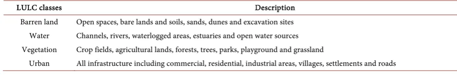
[image:9.595.59.543.418.604.2]A classification scheme had to be established before image classification. By computing average spectra of each class, a spectral characteristic of each land use class in each of the acquired data had been recognized, resulting in a classifica-tion schema comprised of 4 LULC level classes described in Table 2. As hig-hlighted below, a number of classification approaches were evaluated for their effectiveness in large area classification [18].
Figure 4. RGB band combination according to the highest OIF values of (a) TM 1990, (b) TM 2003, and (c) OLI 2016.
Table 2. Classification schema of LULC in the study area.
LULC classes Description
Barren land Open spaces, bare lands and soils, sands, dunes and excavation sites Water Channels, rivers, waterlogged areas, estuaries and open water sources Vegetation Crop fields, agricultural lands, forests, trees, parks, playground and grassland
[image:9.595.53.520.653.730.2]DOI: 10.4236/jgis.2018.101003 66 Journal of Geographic Information System
4.3.1. Unsupervised Classification
A combination of unsupervised classification methods were used to classify the study area. Images were first classified using the Unsupervised Interactive Self- organizing Data Analysis (ISODATA) algorithm to identify spectral cluster formation from image data and convert image data to thematic data. This in-formation contains average spectra for each of the identified LULC stored in a signature file, which in turn makes use of analyst with the help of the ground truth points and first-hand knowledge of the study area to recognize and assign spectrally uniform training data for a subsequent application of different super-vised classification algorithms [7]. This clustering process was repeated several times through much iteration until a threshold was reached and there was no significant change in the cluster statistics or the maximum number of iterations was reached [48]. Clustering processes are highly automated with no direction from the users, so are ideal for large study area application.
4.3.2. Supervised Classification
The data were processed further using different supervised classification algo-rithms after they were classified using an unsupervised ISODATA algorithm. Training samples were first digitized from different representative classes to identify pixels of a single class. Grouping different spectral and spatial classes was done on the basis of LULC classes by utilizing reference data obtained from GCPs; auxiliary information and knowledge-based approaches collected from various resources, as mentioned before, were used to evaluate the statistical sig-nature files of each LULC class [49] and ensure that there was minimal confu-sion of the land use to be mapped [50]. Different supervised classification algo-rithms were then carried out on the Landsat images; the executed algoalgo-rithms in-cluded: Parallelepiped, Minimum distance, Mahalanobis distance, Maximum Likelihood and Support Vector Machine. Several algorithms were applied to iden-tify the best for the study area location.
In order to increase classification accuracy and reduce classification error caused by confusion in spectral response of specific classes, the generalized im-ages were spatially reclassified and refined for classification validation. Spectral confusion occurred due to the fact that several LULC have similar spectral re-sponse with respect to sensor characteristics especially in urban areas [20]. Therefore, data reclassification has to be applied to consolidate different LULC types using the image spatial and contextual properties. Reclassification was car-ried out based on auxiliary data and several GIS functions, for instance: digitiz-ing, overlaying and region of interest (ROI) functionality to produce the last ver-sion of LULC maps for different years.
4.4. Post Classification Smoothing
4.4.1. Accuracy Assessment and Validation
DOI: 10.4236/jgis.2018.101003 67 Journal of Geographic Information System
real world and ensure the reliability of the information derived from LULC maps. Confusion matrices were computed to evaluate the relationship between the reference data used and the resulting classified LULC maps. Confusion ma-trices are one of the most popular ways to evaluate the overall classification ac-curacy providing information about producer’s acac-curacy or errors of omission (percentage of a specific LULC class on the ground which is correctly classified) and user’s accuracy or error of commission (percentage of a certain pixel class on the produced map corresponding to the actual class on the ground) [13] [51]. Percentage of the overall accuracy was computed using the following formula
[12]:
( )
total number of correct samplesOverall accuary % 100
total numer of samples
= × (2)
Congalton (1991) was the first to point out that 250 reference pixels (±5%) are needed to construct the confusion matrix and to estimate the actual mean of ac-curacy assessment [52]. Therefore, 300 randomly selected reference pixels, placed on the classified images, for each time period were generated, representing a spe-cific coordinate of the image. These points, distributed using the stratified ran-dom method, were then listed in two classes, one representing the class or refer-ence values, while the other represented the actual LULC type. The percentage of the actual agreement of the automated classifier over a purely random assign-ment to classes was determined using a non-parametric Kappa coefficient [49] to remove the contribution of correct classification due to chance [18]. The Kappa coefficient for the different classification algorithms was evaluated by the fol-lowing simplified equation [53] [54]:
( )
( )
( )
Kappa 1
P A P E
P E
− =
− (3)
where P(A) is the observed accuracy and P(E) is the chance agreement.
4.4.2. Land Use/Land Cover Change Detection
A multi-date post-classification comparison change detection method was em-ployed to quantify the temporal change in LULC in the area of interest [55]. Three change detection statistics were obtained over time from the independent classified images for this research by conducting cross-tabulation analysis on a pixel-by-pixel basis, i.e. thematic overlay of the classified images [56]. The possi-bilities were (1990-2003), (2003-2016) and (1990-2016) to evaluate the matrix table of “from-to” change information that revealed the main gains and losses in each category of the study site.
4.5. Derivation of Land Surface Indices (NDVI and NDBI)
DOI: 10.4236/jgis.2018.101003 68 Journal of Geographic Information System
radiant temperature [2]. NDBI was first developed [58] to investigate the extent of imperviousness and built-up areas and map these areas, as it can highlight the urban distribution with a typically higher reflectance in the short-wave infrared region band than that of the near-infrared one [59]. NDVI and NDBI were computed using the following formulas from different wavelength regions of the Landsat data: NIR Red NDVI NIR Red − =
+
(4)
SWIR NIR NDBI
SWIR NIR
− =
+ (5)
where NIR, Red and SWIR are the reflectance in the Near-Infrared band (0.76 - 0.9 µm), Red band (0.63 - 0.69 µm) and Short-wave Infrared band (1.55 - 1.75 µm), respectively, for Landsat 5 TM. However, for Landsat 8 OLI these differed slightly: Near-Infrared band (0.85 - 0.88 µm), Red band (0.64 - 0.67 µm) and Short-wave Infrared band (1.57 - 1.65 µm).
4.6. Land Surface Temperature Retrieval from Landsat 5 TM Data
Atmospheric correction was first required to eliminate the atmospheric effect from thermal bands, as the satellite imagery measures the radiance of surface features modified by the atmosphere [9]. Therefore, the Top of Atmospheric (TOA) radiance correction model was applied on Landsat 5 TM imageries for both 1990 and 2003. TOA radiance is a simple model based on the scene calibra-tion data available from the imagery header file. Based on [60], brightness tem-perature from Landsat 5 can be obtained first by the conversion of the digital number of band 6 to Top of Atmospheric (TOA) radiance using the following equation: MAX MIN MIN MAX Cal Cal L L
L Q L
Q
λ λ
λ λ
−
= +
(6)
where Lλ is TOA radiance, LλMAX is highest radiance corresponding to
MAX
Cal
Q (DN = 255), LλMIN is lowest radiance corresponding to QCalMIN (DN = 0), and QCal is the quantized calibrated pixel value of band 6 in DNs.
The thermal band can then be converted from TOA radiance to effective at-sensor brightness temperature under the assumption that the Earth’s surface is a blackbody with a uniform emissivity and includes atmospheric effects using the following expression:
2 sensor 1 ln 1 K T K Lλ = + (7)
where Tsensor is at-satellite temperature in Kelvin, K1 is a calibration constant 1 (W/m2 sr μm), and K
2 is a calibration constant 2 in Kelvin (Table 3).
DOI: 10.4236/jgis.2018.101003 69 Journal of Geographic Information System
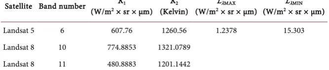
Table 3. Landsat thermal band calibration constants.
Satellite Band number K1
(W/m2 × sr × μm) (Kelvin) K2 (W/m2L × sr × μm) λMAX (W/m2L × sr × μm) λMIN Landsat 5 6 607.76 1260.56 1.2378 15.303 Landsat 8 10 774.8853 1321.0789
Landsat 8 11 480.8883 1201.1442
a Planck surface, the expression to convert the TOA radiance to surface reflec-tance, correcting for solar irradiance, solar zenith and atmospheric effects is [9]:
2 π cos s L d ESUN λ λ λ ρ θ × × =
× (8)
The correct evaluation of LST was constrained to an accurate estimation of surface emissivity. In this work, we considered NDVI to calculate emissivity us-ing the followus-ing formula [61]:
(
)
ln NDVI
a b
ε= + × (9)
where a and b are obtained by regression analysis based on a large dataset [62], a
= 1.0094 and b = 0.047.
Finally, the LST corrected, in Celsius, for spectral emissivity is computed us-ing the followus-ing expression [62]:
( )
( )
sensor sensor
LST C 273.15
1 ln T T λ ε ρ = − × + ×
(10)
where λ is the wavelength of emitted radiance (the average wavelengths = 11.45 µm) [63], ρ= ×h c σ (1.438 × 10⁻² m⋅K) with: σ is Boltzman constant
(1.38 × 10⁻²³ J/K), h is Planck’s constant (6.626 × 10⁻³⁴ J⋅s), and c is the velocity
of light (2.998 × 10⁸ m/s).
4.7. Land Surface Temperature Retrieval from Landsat 8 OLI
In the case of Landsat 8, TOA spectral radiance was computed using the ra-diance rescaling factors corresponding to each band provided in the metadata file using the following equation [44]:
L Cal L
Lλ =M ×Q +A (11)
where ML is the radiance multiplier, QCal is the pixel value in DN and AL is
the radiance additive scaling factor for the bands obtained from the metadata. A web-based atmospheric correction model was used to evaluate surface tem-perature by first converting the previously calculated TOA radiance to sur-face-leaving radiance, taking into account the atmospheric correction of thermal regions of Landsat 8 OLI [64]:
1 up
T d
L L
L λ ε L
τ ε ε
− −
= − ×
DOI: 10.4236/jgis.2018.101003 70 Journal of Geographic Information System
where LT is atmospherically corrected radiance, Lup and Ld are upwelling and
downwelling radiance, respectively (W/m2⋅sr⋅μm), and τ and ε are
transmis-sivity and emistransmis-sivity, respectively. These parameters can be assessed using the Atmospheric Correction Parameter Calculator online tool
(https://atmcorr.gsfc.nasa.gov/). This uses the MODTRAN radiative transfer
code that integrates algorithms to estimate atmospheric global profiles and pa-rameters for a certain date, time, and location as the input [65]. Land surface emissivity was computed according to Equation (9). Even though the emissivity was calculated via NDVI in both Landsat 5 TM and Landsat 8 OLI, it was also preferable to use the same emissivity model for both Landsat datasets, hence avoiding uncertainty in the change in LST. Additional emissivity models intro-duced by [66] were also applied; however, results obtained corresponding to Equation (9) were considered the most reliable and the closest to the real life af-ter validation, with only small differences found between the models.
Thermal Infrared bands of Landsat 8 OLI are converted from spectral ra-diance to effective at-sensor brightness temperature by converting the rara-diance using the inverse Landsat Plank’s law [60]:
2
1
273.15
ln 1
T
K BT
K L
= −
+
(13)
where K1 is the band specific-thermal conversation constant 1 (W/m2 sr μm),
and K2 is a calibration constant 2 in Kelvin (Table 3). Lastly, the emissivity-
corrected LST, in Celsius, was retrieved using Equation (10) with the replace-ment of BT instead of TSensor.
5. Results and Discussion
5.1. Spatial Distribution and Accuracy Assessment of LULC
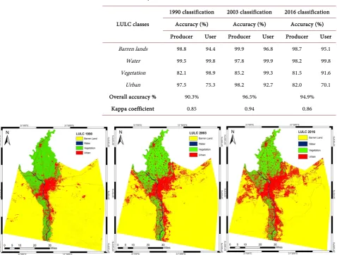
The Support Vector Machine (SVM) and maximum likelihood algorithms pro-vided higher overall accuracy and kappa coefficients than other supervised clas-sification algorithms (Table 4). Utilizing this observation, image processing and spectral characteristics, the final product combining the unsupervised and su-pervised classifications in which the spatial distribution and patterns of the LULC changes and persistence for the years 1990, 2003 and 2016, are shown in
Figure 5. Spatial distribution patterns reveal that the area was dominated by deserts and barren lands, vegetation in the northern region and urban cover in the middle. Due to the heterogenic and dense vegetation cover in the north cen-tral part of the study region, we could not obtain higher overall accuracies than the ones presented, even after repeated classification with different algorithms.
DOI: 10.4236/jgis.2018.101003 71 Journal of Geographic Information System
[image:15.595.211.540.189.308.2]and water were classified relatively accurately, approximately 98% or higher. The overall classifications in 2003 and 2016 are higher because of the availability of more detailed and higher resolution aerial reference images. Meanwhile, the use of OIF and enhancement techniques prior to classification increased the overall accuracy by 15% to 20%.
Table 4. Accuracy assessment of different supervised classification algorithms used for LULC maps in GCR.
Classification algorithms Overall accuracy (%) Kappa coefficient 1990 2003 2016 1990 2003 2016 Minimum distance 86.7 90.6 86.6 0.78 0.84 0.79
[image:15.595.61.540.331.693.2]Parallelepiped 80.8 86.1 78.9 0.71 0.78 0.70 Mahalanobis 87.1 92.7 89.0 0.80 0.88 0.83 Maximum likelihood 88.3 95.9 88.4 0.82 0.93 0.81 Support vector machine 90.3 96.5 94.9 0.85 0.94 0.86
Table 5. Accuracy assessment of the LULC classification results for GCR.
LULC classes
1990 classification 2003 classification 2016 classification Accuracy (%) Accuracy (%) Accuracy (%) Producer User Producer User Producer User Barren lands 98.8 94.4 99.9 96.8 98.7 95.1 Water 99.5 99.8 97.8 99.9 98.2 99.8 Vegetation 82.1 98.9 85.2 99.3 81.5 91.6 Urban 97.5 75.3 98.2 92.7 82.0 70.1
Overall accuracy % 90.3% 96.5% 94.9%
Kappa coefficient 0.85 0.94 0.86
DOI: 10.4236/jgis.2018.101003 72 Journal of Geographic Information System
5.2. Land Use/Land Cover Change Detection
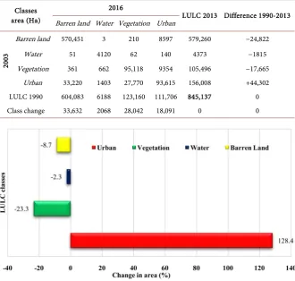
[image:16.595.208.540.225.362.2]Change detection statistics were computed from each consecutive pair of LULC maps (1990-2003 and 2003-2016), and the results of these changes are furnished in Table 6 and Table 7. This shows the nature of change with respect to each class obtained from a matrix algorithm. Change detection analysis results show a sharp growth of 128% in the urban class during the 26-year period (1990-2016) (Figure 6). Significant differences appear to be related to barren land and vege-tation land cover classes. Vegevege-tation cover was reduced by 17,665 ha (14.3%)
Table 6. “From-to” LULC change detection statistics for 1990-2003 for GCR in hectare.
Classes area (Ha)
2003
LULC 2013 Difference 1990-2013 Barren land Water Vegetation Urban
19
90
Barren land 598,519 2 134 5428 604,083 −30,669 Water 25 4231 945 987 6188 +1710 Vegetation 829 95 115,167 7069 123,160 −14,432
[image:16.595.208.539.393.707.2]Urban 35,379 149 21,346 54,832 111,706 +43,387 LULC 1990 634,752 4478 137,592 68,316 845,137 0 Class change 36,233 247 22,426 13,484 0 0
Table 7. “From-to” LULC change detection statistics for 2003-2016 for GCR in hectare.
Classes area (Ha)
2016
LULC 2013 Difference 1990-2013 Barren land Water Vegetation Urban
20
03
Barren land 570,451 3 210 8597 579,260 −24,822
Water 51 4120 62 140 4373 −1815
Vegetation 361 662 95,118 9354 105,496 −17,665 Urban 33,220 1403 27,770 93,615 156,008 +44,302 LULC 1990 604,083 6188 123,160 111,706 845,137 0 Class change 33,632 2068 28,042 18,091 0 0
DOI: 10.4236/jgis.2018.101003 73 Journal of Geographic Information System
during 2003-2016 as compared to 14,432 ha (10.5%) during 1990-2003. Mean-while, the barren land had a major decline of 30,669 ha (4.8%) and 24,822 ha (4.1%) during the two periods of 1990-2003 and 2003-2016, respectively, with a total amount of 55,491 ha during the entire period. These massive changes are related to desert-urbanization activities and construction of new housing devel-opments, initiated by the Egyptian government in the early 1980s and that have since been accelerated [7]. This increasing trend in urbanization enhances the effect of human interference and reinforces that socio-economic forces are the main stimulus on these anthropogenic land changes, specifically around streams coming out from the Nile River. However, the reduction of vegetation cover and agricultural area, especially for urbanization purposes, illustrates the poor plan-ning of farmland protection laws and the ignoring of environmental and ecolog-ical legislation implemented in the urban master plan. Water bodies, on the oth-er hand, increased in area during 1990-2003, and then decreased again, due to the use of surrounding land for agriculture. Results obtained from this study were similar to that evaluated by [67]. They used three satellite images (1984, 2003 and 2014) to produce three LULC maps in GCR using the SVM algorithm. Results indicated that 13% of the vegetation was lost to urban areas between the period of 1984 to 2003, and 12% was lost between 2003 and 2014. However, only 3% of desert became urban areas in the first period, jumping to 5% between 2003 and 2014.
In order to better understand these “From-to” relationships, further GIS and statistical analyses were conducted. A post-classification comparison was con-ducted through cross-tabulation GIS modules to overlay the two LULC maps (1990 and 2016) to produce a LULC change detection map pointing out the spa-tial pattern of change for the 26-year timespan (Figure 7). Figure 8 and Table 8
show the percentage of different land covers in the GCR for the three time pe-riods considered in this study. Results highlighted from these analyses showed two clearly recognizable trends; a) barren land and vegetation cover declined gradually and b) urban area increased drastically and rapidly (at the rate of 128% as mentioned before). The conversion patterns between different land cover classes to urban land cover are illustrated in Figure 9. This reveals that barren land was the main contributor in shaping urban area by an amount of 8.70% followed by vegetation land cover by a rate of 7.73% within the 26-year timespan (1990-2016). This emphasizes the importance of RS in conjunction with GIS in the study of LULC change detection providing essential information about the dynamic nature and patterns of spatial change of land cover.
DOI: 10.4236/jgis.2018.101003 74 Journal of Geographic Information System
[image:18.595.111.487.461.703.2]Figure 7. Land cover conversion in GCR from 1990 to 2016.
Table 8. Change areas of LULC classes in the three time periods 1990, 2003 and 2016 in the study area.
LULC area 1990 2003 2016
Hectares Hectares Hectares
Barren land 634,752 604,083 579,260
Water 4478 6188 4373
Vegetation 137,592 123,160 105,496
Urban 68,315 111,706 156,008
[image:18.595.109.488.461.704.2]DOI: 10.4236/jgis.2018.101003 75 Journal of Geographic Information System
Figure 9. Contribution to the net change in the urban land cover in GCR (Area percen-tage %).
texture, especially during the period of 2003-2016. These are related to the estab-lishment and implementation of new settlements, industries and communities at the expense of desert land that relies on surface water from the Nile River, for instance, El-Obour city and 10th of Ramadan cities to the east of Cairo, and 6 of
October City in the western part. In general, these intense expansions occurred to accommodate the increasing population which caused the need for creating new jobs and maintaining food security, and is confirmed by Census data dis-cussed in section 2 (Figure 2).
5.3. Land Surface Temperature (LST) Change and the
Relationship with Land Use/Land Cover (LULC) Change
DOI: 10.4236/jgis.2018.101003 76 Journal of Geographic Information System
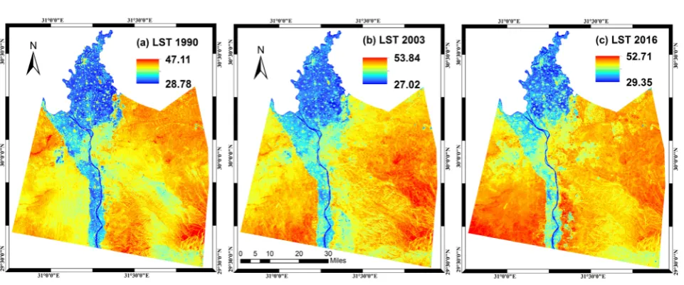
[image:20.595.207.540.321.387.2]Figure 10. Spatial distribution of GCR LST for the years (a) 1990, (b) 2003 and (c) 2016.
Table 9. Cross validation of the estimated LST from Landsat data with meteorological data for GCR.
Acquisition date Satellite LST estimation Meteorological stations Difference
Aug. 4th 1990 38.4 38 0.4
Aug. 8th 2003 40.6 36 4.6
Aug. 11th 2016 42.1 39 3.1
Table 10. Average LST distribution (˚C) over different LULC classes in GCR for the years 1990, 2003 and 2016.
LULC classes
1990 2003 2016 Average
change in LST (1990-2016) Range Mean
LST Dev St. Mean LST Dev St. Mean LST Dev St.
Barren land 39.81 1.48 42.49 1.85 43.69 1.43 3.88 0.15
Water 30.59 2.28 31.33 2.17 32.89 2.50 2.30 0.09 Vegetation 33.05 2.29 34.00 2.32 36.00 2.82 2.95 0.11 Urban 36.83 2.11 38.14 2.24 41.74 2.48 4.91 0.19
used to calibrate the distribution of LST in such dense places as GCR. Different algorithms for LST evaluation from Landsat were applied in this study to obtain accurate results. The calibration of LST should be refined with more data and in situ measurements of LST in future studies, as suggested by [32].
[image:20.595.210.539.429.559.2]DOI: 10.4236/jgis.2018.101003 77 Journal of Geographic Information System
had been converted from other land cover types [9]. Results revealed that the highest maximum and mean LST were associated with barren land (mean value of 39.81˚C to 43.69˚C) and high density urban areas (mean value of 36.83˚C to 41.47˚C), followed by vegetation (mean value of 33.05˚C to 36˚C) and, lastly, water cover (mean value of 30.59˚C to 32.89˚C), in all three periods. Due to the urban-warming effect and rapid urban growth in GCR, urban areas, such as in-dustrial districts and commercial centers in the eastern and western side of Cai-ro, experienced an increase in LST by 4.91˚C over the entire period. This implies that these noticeable increases were due to high emissions of pollutants and multiple artificial heat sources, and the replacement of native vegetation areas that reduce the amount of heat stored through transpiration with other non- transpiring and non-evaporating surfaces such as concrete, metals and stones. These high density building surfaces experience high radiance temperatures, confirming the phenomena of urban-warming effect in which man-made mate-rials in dense urban areas alter the superficial temperature and strongly link the urban category to higher LST in GCR.
It is also noted that vegetation cover showed the highest standard deviation values, reflecting the heterogeneous and complex nature of the vegetation cover with a wide range of surface radiant temperature. On the other hand, barren lands exhibited the lowest standard deviation due to the dry nature of these sur-faces and a lack of wide variation in surface radiant temperature.
[image:21.595.211.540.610.735.2]Table 11 shows how the newly formed lands reacted with regard to LST after transformation, excluding water cover that accounts for less than 1% of the study area. It can be clearly noted that the newly developed barren lands and urban areas have measured higher temperatures when transformed from vegeta-tion cover with rates of 2.60˚C and 2.06˚C, respectively. On the other hand, ve-getation cover tends to decrease the radiant LST in the conversion from either urban areas (1.90˚C) or barren lands (0.43˚C). Note that the transformation be-tween barren lands and urban areas (and vice versa) had minimal effect on LST. In general, different land covers had different influences on the thermal distri-bution with a different magnitude, and LST acted as an important function of the change in LULC. Therefore, it is vital to increase the green area to strengthen study area protection.
Table 11. Average LST change in different LULC change types from 1990 to 2016 in GCR.
DOI: 10.4236/jgis.2018.101003 78 Journal of Geographic Information System
5.4. Analysis of Land Indices and Relationship with LST
[image:22.595.60.537.313.500.2]Two indices, NDVI and NDBI, as mentioned in section 4.5, were derived to quan-tify the relationship between LST and land indices. The visual depiction of the spatial pattern of both NDVI and NDBI are shown in Figure 11 and Figure 12, respectively. It is observed that higher NDVI values correspond to dense vegeta-tion areas in the central north of GCR, while lower values were observed in ur-ban areas and barren land (Table 12). NDVI values are in the range of −0.525 to 0.79 in 1990, have a mean value of 0.04 and standard deviation of 0.15. These values dropped to −0.444 and 0.681 with a mean of 0.026 and a 0.14 standard deviation in 2003, and gradually decrease to be between −0.528 and 0.681, with a mean of −0.02 and a 0.08 standard deviation in 2016. As documented in the lite-rature [31], higher levels of NDVI were associated with lower values of LST. On the other hand, NDBI values were found to increase over the study period. For 1990, 2003 and 2016, the average NDBI was −0.043, −0.039 and 0.021, respec-tively. In general, decreasing surface transpiration through the reduction green
[image:22.595.63.540.520.705.2]Figure 11. Spatial distribution of NDVI for the years (a) 1990, (b) 2003 and (c) 2016.
DOI: 10.4236/jgis.2018.101003 79 Journal of Geographic Information System
Table 12. Mean values of NDVI and NDBI for the years 1990, 2003 and 2016 for GCR.
LULC classes 1990 2003 2016
NDVI NDBI NDVI NDBI NDVI NDBI Barren lands −0.029 0.050 −0.040 0.049 −0.061 0.077
[image:23.595.208.539.237.324.2]Water −0.147 −0.429 −0.042 −0.047 0.071 −0.235 Vegetation 0.467 −0.444 0.357 −0.043 0.255 −0.226 Urban 0.033 −0.075 0.025 −0.054 0.008 −0.015
Table 13. Correlation coefficient matrix from the indices and LST for the years 1990, 2003 and 2016 for GCR.
1990 2003 2016
LST NDVI NDBI LST NDVI NDBI LST NDVI NDBI LST 1.00 −0.87 0.91 1.00 −0.86 0.90 1.00 −0.88 0.89 NDVI −0.87 1.00 −0.96 −0.86 1.00 −0.96 −0.88 1.00 −0.98 NDBI 0.91 −0.96 1.00 0.90 −0.96 1.00 −0.98 0.89 1.00
Table 14. Pearson’s correlation between LST and two indices at 0.05 significance level.
1990 2003 2016
R2 Root MSE P-value R2 Root MSE P-value R2 Root MSE P-value LST vs. NDVI 0.7566 1.825 <0.0001 0.7419 2.323 <0.0001 0.7821 1.902 <0.0001 LST vs. NDBI 0.8310 1.520 <0.0001 0.8033 2.028 <0.0001 0.7980 1.832 <0.0001
canopy cover and increasing impervious surfaces modified thermal behavior and were essential to the reduced value of NDVI and increased NDBI. This pattern can be clearly seen in Table 13 and Table 14, showing the statistical analysis and the Pearson’s correlation coefficient between the indices and LST at a 0.05 signi-ficance level. The results revealed that NDVI was negatively correlated with LST, indicating the impact of green cover on LST is negative, in which the more green areas, the weaker LST will be (Figure 13). In comparison, NDBI presents a high positive correlation coefficient with LST over the three time periods of the study. Therefore, urban areas can strengthen urban heat effects and increase LST [32]
(Figure 14). It was interesting to note that the high negative correlation between NDVI and NDBI in the three years could be explained by the action of estab-lishing urban settlements in favor of green cover.
[image:23.595.206.538.356.425.2]DOI: 10.4236/jgis.2018.101003 80 Journal of Geographic Information System
[image:24.595.60.541.220.339.2]Figure 13. Correlation between NDVI and LST for the years (a) 1990, (b) 2003 and (c) 2016 for GCR.
Figure 14. Correlation between NDBI and LST for the years (a) 1990, (b) 2003 and (c) 2016 for GCR.
Figure 15. Correlation among LST, NDVI and NDBI from a West/East profile in 2016 imagery.
relationship among the variables as shown in Equation (14), with a correlation coefficient of R2 = 0.80, p < 0.001, and Root MSE = 1.82 at a 0.05 significance
level.
LST= −6.79 NDVI× +21.60 NDBI× +41.26 (14)
The finding of Equation (14) showed a higher correlation coefficient in the multivariate linear regression than those of simple linear ones for the same year (R2 = 0.78 for LST-NDVI and R2 = 0.79 for LST-NDBI).
Pearson’s Correlation Coefficient between LST, NDVI and NDBI by Different LULC Types
[image:24.595.59.538.372.522.2]DOI: 10.4236/jgis.2018.101003 81 Journal of Geographic Information System
Table 15. Pearson’s correlation between LST and NDVI by LULC type at 0.05 significance level.
LULC classes
LST/NDVI (1990) LST/NDVI (2016)
R2 Regression functions Correlation RMSE R2 Regression functions Correlation RMSE Barren
lands 0.008 LST= −6.58 NDVI× +39.8 −0.090 0.93 0.105 LST= −34.45 NDVI× +41.9 −0.325 1.54 Water 0.081 LST=4.67×NDVI+30.5 0.284 1.16 0.108 LST= −28.92×NDVI+34.0 −0.329 1.36
Vegetation 0.385 LST= −9.69×NDVI+36.4 −0.620 1.34 0.349 LST= −20.15 NDVI× +38.5 −0.590 1.79
Urban 0.355 LST= −7.19×NDVI+37.7 −0.596 2.14 0.392 LST= −30.64×NDVI+40.30 −0.626 2.02
Table 16. Pearson’s correlation between LST and NDBI by LULC type at 0.05 significance level.
LULC classes
LST/NDBI (1990) LST/NDBI (2016)
R2 Regression functions Correlation RMSE R2 Regression functions Correlation RMSE Barren lands 0.009 LST= −3.04×NDBI+40.2 −0.097 0.93 0.107 LST=27.55 NDBI× +41.9 0.327 1.54
Water 0.013 LST=1.68 NDBI× +30.5 0.114 1.20 0.280 LST=14.16×NDBI+35.2 0.529 1.24
Vegetation 0.483 LST=9.12×NDBI+36.9 0.695 1.23 0.381 LST=14.67×NDBI+38.7 0.618 1.75
Urban 0.435 LST=13.58 NDBI× +38.2 0.660 2.01 0.423 LST=20.60×NDVI+40.31 0.652 1.96
LST/NDBI (Table 16) for LULC, pixel-by-pixel, in 1990 and 2016.
Results showed that the correlation between LST and NDVI were all negative in both 1990 and 2016 except for water coverage in 1990, likely due to lower amounts of pollutants in the 1990 water. However, the lowest negative correla-tion was found on barren lands in 1990 due to the high area coverage in the study region. On the other hand, the highest negative coefficient of the regres-sion function was found to be in vegetation covers (−0.620) and dropped slightly for urban cover (−0.596). In 2016, barren area still showed the lowest negative correlation, however urban cover experienced the highest correlation coefficient (0.652), slightly higher than that of the vegetation one. Results of this analysis are consistence with other studies discussing the relationship between LST and NDVI [68] [69]. This indicates that by increasing NDVI, the LST of both vegeta-tion and urban areas decreases more quickly than that of barren land cover.
However, the NDBI index showed a positive correlation with all LULC types except for barren lands in 1990 which had negative or almost no correlation with LST. Similar to NDVI, the highest coefficient was related to vegetation in 1990 and urban cover in 2016. In general, the correlation coefficient between LST and land surface indices for the whole study area showed a higher correlation than in the case of using indices as indicators for LST according to each LULC type. However, the moderate relationship obtained for each LULC by surface indices and LST can provide important information for preliminary studies; for exam-ple, they can be simply used as proxies for temperature and for better planning by policy makers in large areas.
6. Conclusions
[image:25.595.55.541.224.320.2]mon-DOI: 10.4236/jgis.2018.101003 82 Journal of Geographic Information System
itor the spatial and temporal change of LULC and to study the impact of rapid urbanization on land surface temperature in the GCR in Egypt. Three Landsat dates, TM 1990, TM 2003 and OLI 2016, were acquired at the same time of the season (summer) due to the availability of reference data and to keep the weath-er factor as constant as possible. The study showed the effectiveness of the re-mote sensing techniques in conjunction with GIS to enable us to delineate the urban expansion due to the establishment of new settlements and to produce an accurate landscape change map in the study area. Different image enhance-ments, atmospheric correction, information extraction techniques, and unsuper- vised and supervised classification algorithms were performed on each Landsat image to ensure accurate image classification and LULC mapping. This revealed that SVM and maximum likelihood gave higher accuracies with rates of 90.3%, 96.5% and 94.9% for the years 1990, 2003 and 2016, respectively. The post-clas- sification comparison change detection method was employed to quantify the spatial change of land cover units. In addition, statistical “from-to” information was applied to quantify the magnitude of change through the entire 26-year time- span. Results demonstrated the most distinct change was related to vegetation cover that drastically decreased by an amount of 32,097 ha (23.3%) from 1990 to 2016. In the same time period, significant reduction in barren land by 55,491 ha (8.70%) occurred. On the other hand, urban areas, due to the construction of new industrial and commercial settlements, showed a considerable increase by 87,689 ha (128.3%), particularly in the central and northern parts of the study area around water resources. These two land covers, barren lands and vegetation, were the main contributors to form new urban areas.
DOI: 10.4236/jgis.2018.101003 83 Journal of Geographic Information System
to settlement expansion resulting in a large amount of waste heat in turn affect-ing the surface energy budget.
Results from remote sensing studies show that LST and land surface indices, NDVI and NDBI together can identify the pattern of temporal variation and spatial distribution in urban thermal environments. The highest NDVI was found in vegetated areas while the highest NDBI was found in barren lands and urban areas. Statistical analysis showed a strong inverse relationship between LST and NDVI in contrast to a high positive one between LST and NDBI along different profiles in the study areas. These relationships dropped in the case of quantitative analysis among LST, LULC pattern and land surface indices. By way of conclusion, the study area reveals comparatively higher LST and NDBI, and lower NDVI over the period of study. These findings recommend the establish-ment of measures that can mitigate the strong effect of increasing LST on sus-tainable developments, population density control that is not limited to hori-zontal growth only, green coverage improvements like parks and gardens, and roof top area cultivation with horticultural plants that can alleviate the effect of LST. More multi-date images from the same season are also recommended to be investigated and evaluated, in a manner of providing more evidence of the thermal behavior on urban areas for better understanding of the impact of urba-nization on LST. Moreover, RS satellite images are likely to be affected by cloud cover and other atmospheric effects, in addition to surface roughness, that in turn affect the DN values and therefore, it is highly recommended for future work that the integration of RS imageries from different sources with more land surface meteorological data be explored, and more attention on surface rough-ness be considered for more accurate results [9].
In general, results proved the potential of multi-temporal Landsat images that can accurately quantify the change pattern in LULC and LST in GCR in Egypt. In addition, the integration of RS and GIS can provide a valuable opportunity for surveying, environmental monitoring and the nature of land cover change. Hence, the information gleaned from the change detection outputs can help in understanding the dynamics of LULC change in order to help policy-makers to predict and plan for future developments in GCR, achieve long-term sustainabil-ity of soil and water resources and its impacts on climate change, and therefore characterize the evolution of urban construction lands.
Acknowledgements
The authors would like to thank Dr. El-Sayed Ewis for his technical support and the Egyptian Government General Scholarship Programme administrated by the Egyptian Cultural and Education Bureau, Washington, DC, USA, for their fi-nancial support of this research.
References
Confe-DOI: 10.4236/jgis.2018.101003 84 Journal of Geographic Information System
rence Series: Earth and Environmental Science, 20, 12056. https://doi.org/10.1088/1755-1315/20/1/012056
[2] Omran, E.S.E. (2012) Detection of Land-Use and Surface Temperature Change at Different Resolutions. Journal of Geographic Information System, 4, 189-203. https://doi.org/10.4236/jgis.2012.43024
[3] Adger, W.N., Arnell, N.W. and Tompkins, E.L. (2005) Successful Adaptation to Cli- mate Change across Scales. Global Environmental Change, 15, 77-86.
https://doi.org/10.1016/j.gloenvcha.2004.12.005
[4] Foley, J.A., Defries, R., Asner, G.P., Barford, C. and Bonan, G. (2005) Global Conse- quences of Land Use. Science (New York, N.Y.), 309, 570-574.
https://doi.org/10.1126/science.1111772
[5] Chen, J., Theller, L., Gitau, M.W., Engel, B.A. and Harbor, J.M. (2017) Urbanization Impacts on Surface Runoff of the Contiguous United States. Journal of Environ-mental Management, 187, 470-481. https://doi.org/10.1016/j.jenvman.2016.11.017 [6] Sahana, M., Ahmed, R. and Sajjad, H. (2016) Analyzing Land Surface Temperature
Distribution in Response to Land Use/Land Cover Change Using Split Window Al-gorithm and Spectral Radiance Model in Sundarban Biosphere Reserve, India.
Modeling Earth Systems and Environment, 2, 81. https://doi.org/10.1007/s40808-016-0135-5
[7] Abdulaziz, A.M., Hurtado, J.J.M. and Al-Douri, R. (2009) Application of Multi-temporal Landsat Data to Monitor Land Cover Changes in the Eastern Nile Delta Region, Egypt. International Journal of Remote Sensing, 30, 2977-2996.
https://doi.org/10.1080/01431160802558675
[8] Ogashawara, I. and Bastos, V. (2012) A Quantitative Approach for Analyzing the Relationship between Urban Heat Islands and Land Cover. Remote Sensing, 4, 3596-3618. https://doi.org/10.3390/rs4113596
[9] Li, L., Tan, Y., Ying, S., Yu, Z., Li, Z. and Lan, H. (2014) Impact of Land Cover and Population Density on Land Surface Temperature: Case Study in Wuhan, China.
Journal of Applied Remote Sensing, 8, 1-19. https://doi.org/10.1117/1.JRS.8.084993 [10] Sheikhi, A., Kanniah, K.D. and Ho, C.H. (2015) Effect of Land Cover and Green Space on Land Surface Temperature of a Fast Growing Economic Region in Malay-sia. Proceedings of SPIE, 9644, 964413. https://doi.org/10.1117/12.2194796 [11] Huyen, N.T., Tu, L.H., Liem, N.D., Tram, V.N.Q., Minh, D.N. and Loi, N.K. (2016)
Assessing Impacts of Land Use and Climate Change on Soil and Water Resources in the Srepok Watershed, Central Highland of Vietnam. Discussion Paper Series- Southeast Asian Regional Center for Graduate Study and Research in Agriculture
(SEARCA),(2016-2). https://doi.org/10.13140/RG.2.2.28700.08326
[12] Pal, S. and Ziaul, S. (2016) Detection of Land Use and Land Cover Change and Land Surface Temperature in English Bazar Urban Centre. The Egyptian Journal of Re-mote Sensing and Space Science, 20, 125-145.
https://doi.org/10.1016/j.ejrs.2016.11.003
[13] Tran, D.X., Pla, F., Latorre-Carmona, P., Myint, S.W., Caetano, M. and Kieu, H.V. (2017) Characterizing the Relationship between Land Use Land Cover Change and Land Surface Temperature. ISPRS Journal of Photogrammetry and Remote Sensing, 124, 119-132. https://doi.org/10.1016/j.isprsjprs.2017.01.001
[14] Mallick, J., Kant, Y. and Bharath, B.D. (2008) Estimation of Land Surface Tempera-ture over Delhi Using Landsat-7 ETM+. J. Ind. Geophys. Union., 12, 131-140. http://www.igu.in/12-3/5javed.pdf
DOI: 10.4236/jgis.2018.101003 85 Journal of Geographic Information System Use/Land Cover Change and Urban Expansion during 1983-2008 in the Coastal Area of Dakshina Kannada District, South India. Journal of Applied Remote Sens-ing, 6, 63576-1. https://doi.org/10.1117/1.JRS.6.063576
[16] Kimuku, C.W. and Ngigi, M. (2017) Study of Urban Heat Island Trends to Aid in Urban Planning in Nakuru County-Kenya. Journal of Geographic Information Sys-tem, 9, 309-325. https://doi.org/10.4236/jgis.2017.93019
[17] Owen, T.W., Carlson, T.N. and Gillies, R.R. (1998) An Assessment of Satellite Re-motely-Sensed Land Cover Parameters in Quantitatively Describing the Climatic Effect of Urbanization. International Journal of Remote Sensing, 19, 1663-1681. https://doi.org/10.1080/014311698215171
[18] Bauer, M.E., Burk, T.E., Ek, A.R., Coppin, P.R., Lime, S.D., Walsh, T.A. and Hein-zen, D.F. (1994) Satellite Inventory of Minnesota Forest Resources. Photogramme-tric Engineering and Remote Sensing, 60, 287-298.
[19] Wilson, E.H. and Sader, S.A. (2002) Detection of Forest Harvest Type Using Mul-tiple Dates of Landsat TM Imagery. Remote Sensing of Environment, 80, 385-396. https://doi.org/10.1016/S0034-4257(01)00318-2
[20] Yang, X. (2002) Satellite Monitoring of Urban Spatial Growth in the Atlanta Met-ropolitan Area. Photogrammetric Engineering and Remote Sensing, 68, 725-734. [21] Yuan, F., Sawaya, K.E., Loeffelholz, B.C. and Bauer, M.E. (2005) Land Cover
Classi-fication and Change Analysis of the Twin Cities (Minnesota) Metropolitan Area by Multitemporal Landsat Remote Sensing. Remote Sensing of Environment, 98, 317- 328. https://doi.org/10.1016/j.rse.2005.08.006
[22] Gilmore, M.S., Wilson, E.H., Barrett, N., Civco, D.L., Prisloe, S., Hurd, J.D. and Chadwick, C. (2008) Integrating Multi-Temporal Spectral and Structural Informa-tion to Map Wetland VegetaInforma-tion in a Lower Connecticut River Tidal Marsh. Re-mote Sensing of Environment, 112, 4048-4060.
https://doi.org/10.1016/j.rse.2008.05.020
[23] Esam, I., Abdalla, F. and Erich, N. (2012) Land Use and Land Cover Changes of West Tahta Region, Sohag Governorate, Upper Egypt. Journal of Geographic Infor- mation System, 4, 483-493. https://doi.org/10.4236/jgis.2012.46053
[24] Ozesmi, S.L. and Bauer, M.E. (2002) Satellite Remote Sensing of Wetlands. Wet-lands Ecology and Management, 10, 381-402.
https://doi.org/10.1023/A:1020908432489
[25] Butt, A., Shabbir, R., Ahmad, S.S. and Aziz, N. (2015) Land Use Change Mapping and Analysis Using Remote Sensing and GIS: A Case Study of Simly Watershed, Is-lamabad, Pakistan. The Egyptian Journal of Remote Sensing and Space Science, 18, 251-259. https://doi.org/10.1016/j.ejrs.2015.07.003
[26] Cohen, W.B., Fiorella, M., Gray, J., Helmer, E. and Anderson, K. (1998) An Efficient and Accurate Method for Mapping Forest Clearcuts in the Pacific Northwest Using Landsat Imagery. Photogrammetric Engineering & Remote Sensing, 64, 293-300. [27] Butt, A., Shabbir, R., Aziz, N. and Nawaz, M. (2015) Land Cover Classification and
Change Detection Analysis of Rawal Watershed Using Remote Sensing Data. Jour-nal of Biodiversity and Environmental Sciences, 6, 236-248.
[28] Rawat, J.S. and Kumar, M. (2015) Monitoring Land Use/Cover Change Using Re-mote Sensing and GIS Techniques: A Case Study of Hawalbagh Block, District Al-mora, Uttarakhand, India. The Egyptian Journal of Remote Sensing and Space Sciences, 18, 77-84. https://doi.org/10.1016/j.ejrs.2015.02.002
DOI: 10.4236/jgis.2018.101003 86 Journal of Geographic Information System [30] Bayarjargal, Y., Karnieli, A., Bayasgalan, M., Khudulmur, S., Gandush, C. and
Tucker, C.J. (2006) A Comparative Study of NOAA-AVHRR Derived Drought In-dices Using Change Vector Analysis. Remote Sensing of Environment, 105, 9-22. https://doi.org/10.1016/j.rse.2006.06.003
[31] Sun, D. and Kafatos, M. (2007) Note on the NDVI-LST Relationship and the Use of Temperature-Related Drought Indices over North America. Geophysical Research Letters, 34, 1-4. https://doi.org/10.1029/2007GL031485
[32] Liu, L. and Zhang, Y. (2011) Urban Heat Island Analysis Using the Landsat TM Da- ta and ASTER Data : A Case Study in Hong Kong. Remote Sensing, 3, 1535-1552. https://doi.org/10.3390/rs3071535
[33] Youneszadeh Jalili, S. (2013) The Effect of Land Use on Land Surface Temperature in the Netherlands. GEM Thesis Series, Lund University, Lund.
[34] Ahmed, B., Kamruzzaman, M., Zhu, X., Rahman, M.S. and Choi, K. (2013) Simula- ting Land Cover Changes and Their Impacts on Land Surface Temperature in Dha-ka, Bangladesh. Remote Sensing, 5, 5969-5998. https://doi.org/10.3390/rs5115969 [35] Rasul, A., Balzter, H., Smith, C., Remedios, J., Adamu, B., Sobrino, J.A. and Weng,
Q. (2017) A Review on Remote Sensing of Urban Heat and Cool Islands. Land, 6, 38-47. https://doi.org/10.3390/land6020038
[36] Zaki, R., Zaki, A. and Ahmed, S. (2011) Land Use and Land Cover Changes in Arid Region: The Case New Urbanized Zone, Northeast Cairo, Egypt. Journal of Geogra- phic Information System, 3, 173-194. https://doi.org/10.4236/jgis.2011.33015 [37] Shahin, M. (1990) Impacts of Urbanization of the Greater Cairo Area on the
Groundwater in the Underlying Aquifer. Hydrological Processes and Water Man-agement in Urban Areas, 198, 243-249.
[38] Khoder, M.I. (2009) Diurnal, Seasonal and Weekdays-Weekends Variations of Ground Level Ozone Concentrations in an Urban Area in Greater Cairo. Environ-mental Monitoring and Assessment, 149, 349-362.
https://doi.org/10.1007/s10661-008-0208-7
[39] El-Batran, M. and Arandel, C. (1998) A Shelter of Their Own: Informal Settlement Expansion in Greater Cairo and Government Responses. Environment and Urbani- zation, 10, 217-232. https://doi.org/10.1177/095624789801000109
[40] CAPMAS (2017) Greater Cairo Region Popoulation. http://www.capmas.gov.eg/ [41] U. S. Geological Survey (2016) Earth Explorer. https://earthexplorer.usgs.gov/ [42] Open Street Map (2016) Road Networks.
https://www.openstreetmap.org/#map=12/30.0550/31.2376 [43] Digital Globe (2017) Image Finder. https://browse.digitalglobe.com
[44] Zanter, K. (2016) Landsat 8 (L8) Data Users Handbook. LSDS-1574 Version 2, 1- 106.
[45] VIS, I. (2009) ENVI Atmospheric Correction Module: QUAC and FLAASH User’s Guide. Module Version 4, 1-44.
[46] Chavez, P., Berlin, G. and Sowers, L. (1982) Statistical Method for Selecting Landsat MSS Ratios. Journal of Applied Photographic Engineering, 8, 23-30.
[47] Qaid, A.M. and Basavarajappa, H.T. (2008) Application of Optimum Index Factor Technique to Lansat-7 Data for Geological Mapping of North East of Hajjah, Ye-men. American-Eurasian Journal Scientific Research, 3, 84-91.
https://doi.org/10.1007/s10661-012-2631-z
Shan-DOI: 10.4236/jgis.2018.101003 87 Journal of Geographic Information System non’s Entropy Index. ISPRS—International Archives of the Photogrammetry, Re-mote Sensing and Spatial Information Sciences, July 12-19 2016, 1017-1021. https://doi.org/10.5194/isprs-archives-XLI-B8-1017-2016
[49] Ahmed, B. (2011) Urban Land Cover Change Detection Analysis and Modelling Spatio-Temporal Growth Dynamics Using Remote Sensing and Gis Techniques: A Case Study of Dhaka, Bangladesh. M.Sc. Thesis, University College London, Lon-don. https://doi.org/10.13140/2.1.1413.5364
[50] Gao, J. and Liu, Y. (2010) Determination of Land Degradation Causes in Tongyu County, Northeast China via Land Cover Change Detection. International Journal of Applied Earth Observation and Geoinformation, 12, 9-16.
https://doi.org/10.1016/j.jag.2009.08.003
[51] Lillesand, T.M., Kiefer, R.W. and Chipman, J.W. (2004) Remote Sensing and Image Interpretation. Chap.7 Digital Image Processing. 5th Edition, Vol. 53, Wiley & Sons, New York. https://doi.org/10.1017/CBO9781107415324.004
[52] Congalton, R.G. (1991) A Review of Assessing the Accuracy of Classifications of Remotely Sensed Data. Remote Sensing of Environment, 37, 35-46.
https://doi.org/10.1016/0034-4257(91)90048-B
[53] Gwet, K. (2002) Kappa Statistic Is Not Satisfactory for Assessing the Extent of Agreement between Raters. Statistical Methods for Inter-Rater Reliability Assess-men, 1, 1-6.
[54] Viera, A.J. and Garrett, J.M. (2005) Understanding Interobserver Agreement: The Kappa Statistic. Family Medicine, 37, 360-363.
[55] Ridd, M.K. and Liu, J. (1998) A Comparison of Four Algorithms for Change Detec-tion in an Urban Environment. Remote Sensing of Environment, 63, 95-100. https://doi.org/10.1016/S0034-4257(97)00112-0
[56] Al-Bakri, J.T., Dauqqah, M. and Brewer, T. (2013) Application of Remote Sensing and GIS for Modeling and Assessment of Land Use/Cover Change in Amman/Jor- dan. Journal of Geographic Information System, 5, 509-519.
https://doi.org/10.4236/jgis.2013.55048
[57] Xiong, Y., Huang, S., Chen, F., Ye, H., Wang, C. and Zhu, C. (2012) The Impacts of Rapid Urbanization on the Thermal Environment: A Remote Sensing Study of Guangzhou, South China. Remote Sensing, 4, 2033-2056.
https://doi.org/10.3390/rs4072033
[58] Zha, Y., Gao, J. and Ni, S. (2003) Use of Normalized Difference Built-Up Index in Automatically Mapping Urban Areas from TM Imagery. International Journal of Remote Sensing, 24, 583-594. https://doi.org/10.1080/01431160304987
[59] Alhawiti, R.H. and Mitsova, D. (2016) Using Landsat-8 Data to Explore the Corre-lation between Urban Heat Island and Urban Land Uses. International Journal of Research in Engineering and Technology, 5, 457-466.
https://doi.org/10.15623/ijret.2016.0503083
[60] Chander, G. and Markham, B. (2003) Revised Landsat-5 TM Radiometrie Calibra-tion Procedures and PostcalibraCalibra-tion Dynamic Ranges. IEEE Transactions on Geos-cience and Remote Sensing, 41, 2674-2677.
https://doi.org/10.1109/TGRS.2003.818464
[61] Giannini, M.B., Belfiore, O.R., Parente, C. and Santamaria, R. (2015) Land Surface Temperature from Landsat 5 TM Images: Comparison of Different Methods Using Airborne Thermal Data. Journal of Engineering Science and Technology Review, 8, 83-90.
![Figure 1. Greater Cairo Region (GCR), Egypt: (a) Location map, (b) The study area (Source: (a) ESRI online, (b) Landsat 8 Pan-Sharpened with DEM from Shuttle Radar Topography Mission (SRTM) [41])](https://thumb-us.123doks.com/thumbv2/123dok_us/9989707.499254/5.595.124.540.489.694/figure-greater-location-landsat-sharpened-shuttle-topography-mission.webp)