Assessment of the release of atomic Na from a burning black liquor droplet using quantitative PLIF

1 Title: Assessment of the release of atomic Na from a burning black liquor droplet using quantitative PLIF

Authors: Woei L. Saw a, Graham J. Nathan a, Peter J. Ashman b, Zeyad T. Alwahabi b

Affiliations: Centre for Energy Technology, The Environment Institute, Schools of aMechanical and bChemical Engineering,

The University of Adelaide,

South Australia 5005

Australia

Type of article: Full-length article

Corresponding Author: Mr. Woei L Saw

School of Mechanical Engineering The University of Adelaide

South Australia 5005 Australia

Telephone: +61 8 8303 3177 Facsimile: +61 8 8303 4367

2 Abstract

The quantitative measurement of atomic sodium (Na) release, at high concentration, from a burning black liquor droplet has been demonstrated using a planar laser-induced fluorescence (PLIF) technique, corrected for fluorescence trapping. The local temperature of the particle was measured to be approximately 1700˚C, at a height of 10 mm above a flat flame burner. The PLIF technique was used to assess the temporal release of atomic Na from the combustion of black liquor and compare it with the Na concentration in the remaining smelt. A first-order model was made to provide insight using a simple plug-flow reactor model based on the independently measured concentration of residual Na in the smelt as a function of time. This model also required the dilution ratio of the combustion products in the flat flame entrained into the plume gas from the black liquor particle to be estimated. The key findings of these studies are: (i) the peak concentration of atomic Na from the combustion of the black liquor droplets is around 1.4 ppm; (ii) very little atomic Na is present during the drying, devolatilisation or char combustion stages; and (iii) the presence of atomic Na during smelt phase dominates over that from the other combustion stages.

3 1. Introduction

Black liquor is the by-product of the Kraft pulping process. It consists of both inorganic pulping chemicals and organic components of wood, mainly lignin [1]. Black liquor is an important source of renewable fuel within the pulp and paper industry. It has a very high Na concentration, approximately 20 wt% (dry), compared with other industrial fuels such as coal and wood, in which it typically spans 0.01–5 wt% (dry). Black liquor is conventionally burned in Kraft recovery boilers to recover pulping chemicals and energy. However, it is also being considered as a feedstock for alternative transport fuel. The black liquor gasification for motors fuels production (BLGMF) is presently under development with a view to replacing conventional recovery boilers. This process converts black liquor to biomass-based methanol and dimethyl-ether (DME) [2]. At present, no measurements are available of the concentration of Na in the plume of a burning black liquor droplet, or of its temperature history. The present investigation aims to meet this need.

The release of Na during the combustion of black liquor is a significant source of fume formation in a recovery boiler. This fume mainly consists of sodium sulphate (Na2SO4) and sodium carbonate (Na2CO3) and is deposited on the surface of heat

4 The combustion of a single black liquor droplet is a process that can be divided into the four stages of drying, devolatilisation, char combustion and smelt oxidation [4]. Many studies on the release of Na from black liquor combustion have been conducted by the analysis of the Na left in the residue. Li and van Heiningen [5] have proposed that most of the vaporised Na is released during the char combustion stage due to the reduction of Na2CO3 bycarbon. A study by Cameron [6] has suggested that a major

source of fume could be the significant amount of Na vapour released due to the oxidation of sodium sulphide (Na2S) by Na2CO3. Kauppinen et al. [7] used several

different reactors and measuring devices and concluded that about 10% of Na is released during pyrolysis from the droplet by fragmentation, as has also been proposed by Verrill et al. [8]. Other researchers have used the chemical equilibrium approach to predict fume formation in the lower furnace. One of these studies, by Pejryd and Hupa [9], has suggested that the major gas-phase Na species within this region are atomic Na and sodium hydroxide (NaOH), which agrees with Borg et al. [10]. A recent study conducted by Saw et al. [11] using the equilibrium calculations to model the distribution of the Na species from the combustion of a black liquor particle in a flat flame also agrees with the previous studies.

5 Previous studies of atomic Na in flames have been conducted using point measurements of laser-induced fluorescence (LIF) to determine the concentration [12–13] and to assess the complex chemistry of Na in flame at various gas conditions [13]. Those measurements, however, do not allow fluxes to be obtained. Later, two-dimensional imaging of the release of atomic Na from a burning black liquor droplet in a flat flame has been undertaken by Saw et al. [14] using planar laser-induced fluorescence (PLIF). However those data only provide qualitative trends of atomic Na concentration. More recently the quantitative measurement of atomic Na has been performed, in the plume of a burning coal particle, in our laboratory by van Eyk et al. [15]. This work established a relationship between the number density of atomic Na and the measured fluorescence signal by a calibration against a known concentration of Na solution. The number density of atomic Na was determined by the Beer-Lambert law and the fluorescence signal was measured directly from the Na plume using an intensified charge-coupled device (ICCD) camera [15]. However, the concentration of Na in coal is much less than in black liquor. The maximum concentration of atomic Na for which quantitative data could be obtained was 80 ppb, which was limited by the seeding approach and the large area of the flat flame burner. Hence, the calibration technique cannot be applied directly to black liquor.

6 gas components present in a flame such as, N2, CO2 and O2 reduces the PLIF signal

[17]. Hence, a new approach is needed to enable quantitative measurement of concentrations found in the plume of a black liquor droplet. This requires firstly the development of an iterative method to correct for fluorescence trapping, IFT. This

correction was obtained by adapting the correction method developed by Choi and Jensen [18] to correct the measured laser induced incandescence (LII). However, such a correction requires independent verification. To meet this need, the present investigation aims are therefore: i) to develop a method to allow quantitative measurement of atomic Na at concentration of order 1 ppm in the plume of a burning black liquor droplet using a simultaneous absorption and fluorescence technique with a correction method; ii) to provide further insight into the release of Na from black liquor during combustion by developing a CHEMKIN model that incorporates Na data from the smelt analysis; and iii) to cross check the measurements and the model by comparing them with each other.

2. Experimental Technique

A sample of black liquor from a Swedish pulp mill, shown in Table 1, was used for the measurements. The black liquor was burned in the flame provided by a flat flame burner at two flame conditions, fuel lean (Øb = 0.9) and fuel rich (Øb = 1.25). Note

that the symbol Øb denotes the equivalence ratio of the burner gases alone, which

7 black liquor (10 mg) was carefully applied to a loop (3 mm diameter) at the tip of a platinum wire (0.5 mm diameter). The loop with the black liquor droplet was placed about 10 mm above the tip of the flat flame burner, using a retort stand.

The flat flame burner comprised a matrix of small diffusion flames with the total burner having dimensions of 80 mm × 100 mm. Details of the burner are described elsewhere [15]. The burner was fed with local natural gas as the fuel and the compressed air was supplied by the laboratory compressor. The total flow rate of fuel and air to the burner was 65.8 L/min (STP). The laser sheet was aligned perpendicular to the burner head and with the centre of the droplet. A co-flow of air was supplied around the flat flame burner to stabilise the flame from flicker. The experiment is thereby repeatable.

2.1. Laser and optical arrangement

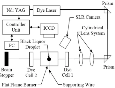
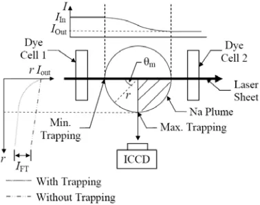
The laser and optical arrangement in the present study is similar to that in Refs. 15 and 19. Two-dimensional images were obtained using PLIF with the arrangement shown in Fig. 1. A tuneable dye laser (Lambda Physik, Scanmate), was pumped by a Nd: YAG (Quantel, Brilliant b) laser. The dye laser was scanned around 16970 cm-1 to excite the D1 and D2 Na lines at 16960.95 cm-1 (589.59 nm) and 16978.22 cm-1 (589

nm), respectively. All the measurements were performed using the D1 line because of

the strong beam absorption observed with the D2 line. The pulse-to-pulse energy

8 intensified CCD camera (Princeton Instruments ICCD-576) aligned orthogonal to the laser sheet. A gate width of 10 ns was selected to minimise noise and background radiation from the flame. Measurements were taken about 15 mm above the black liquor droplet to avoid the scattered light from the particle and the platinum wire. Images were recorded at five images per second.

For absorption measurements, the incoming and outgoing laser intensity was obtained from the two dye cells. It is known that collisional quenching with major species play an important role in LIF [17]. To account for the effects of collisional quenching due to collisions with major species [17], both the PLIF and absorption signals were collected simultaneously using the ICCD camera so that the fluorescence trapping correction will also incorporates the effects of quenching.

A digital single-lens reflex (SLR) camera, directed at the droplet was operated at 3 Hz to measure the history of droplet diameter and identify the stages of combustion simultaneously with the laser measurement of the atomic Na. Note that only the stages of combustion are reported here. To minimise the elastic laser scattering process, a polarisation suppression technique was applied. This was achieved by placing a thin film polariser in the front of the ICCD camera lens. No signal was observed when the polarisation axis of the polariser was set perpendicular to the laser polarisation axis.

2.2. Smelt analysis

9 20, 40, 80, 120, 160, 220 and 240 s for Øb = 1.25. The weight of the hook, together

with the residue, was measured and the weight of the residue determined by subtraction. The hook was transferred to a container filled with 10 ml of distilled water and rinsed for 30 minutes to ensure that all Na salts were dissolved. The Na concentration of each solution was analysed by Inductively Coupled Plasma Atomic Emission Spectrometry (ICP-AES).

2.3. Temperature measurement

The temperature of the flat flame was measured on the centre-line without a burning droplet using a 0.5 mm diameter Type-R (Pt/Pt-13% Rh) thermocouple. The measured temperatures were corrected for radiation losses using the radiation correction equation of Fristrom and Westenberg [20]. The correction was typically 300ºC and the uncertainties were calculated to be ±50ºC.

2.4. Estimation of dilution ratio of combustion products entraining into the plume gas

A method was developed to estimate the diluted atomic Na concentration of the combustion products (from the combustion of the natural gas and air) entrained into the Na plume that is released from the black liquor particle. This method employs the similarity solutions for a fully developed jet flow. It was adapted from the study conducted by Becker et al. [21] on the nozzle-fluid concentration field of a round, turbulent, free jet, taking the plume and the combustion products to be the jet and co-flow, respectively. The constants in the standard laws of decay of the centre line concentration, Cref/C, and growth of the concentration half-radius, b1/2, [21], as shown

10 plume in the region where linear behaviour is closely approximated. Note that Cref

was taken to be the most upstream concentration measurement on the centre-line, which is found approximately 15 mm above the particle.

b1/2 = C1(x – xo) (1)

Cref/C = C2(x – xo)/ro (2)

Here, C1 is the radial jet growth constant, C2 is the axial decay constant, xo is the

virtual origin and ro is the radius of the nozzle based on that of wire loop. A check was

made using the ratio of the cross-sectional area of the droplet plume divided by the cross-sectional area of the burner.

2.5. Model development

A model of Na concentration as a function of dilution by combustion products entrained into the Na plume for Øm = 0.9 and Øm = 1.25 was developed using the Plug

Flow Reactor (PFR) model in CHEMKIN 4.1 with GRI-Mech v3.0 [22] in conjunction with the kinetic data for reactions of Na, H, O and S obtained from Refs. 23, 24 and 25. Note that the symbol Øm denotes the equivalence ratio of the model.

Chlorine (Cl) is not included in the model due to most of the chlorides being vaporised during the devolatilisation and the early stage of the char combustion stages [26]. The calculated Na concentration was then compared with the Single Equilibrium Reactor (SER) model in the similar software. These models, however, can only be considered to be qualitative. The main components of the smelt are Na2CO3 and Na2S

for Øm = 1.25 with the Na2S converted to Na2SO4 under oxidizing conditions [4],

which applies for the Øm = 0.9 case used in this study. These Na salts, Na2CO3, Na2S

andNa2SO4,decompose at 860ºC, 1172ºC and 884ºC, respectively [27], which is well

11 have concluded that these species are relatively unstable molecules in a flame environment [25, 28]. However, the kinetic reactions of Na-S are included in this model.

The composition of the combustion products from the gas burner for both stoichiometries was calculated using the Pre-Mixed Burner model with GRI-Mech v3.0 [22]. The gas released from the particle was assumed to be the difference between the initial and residual mass of the particle at the specific exposure time. In these calculations, the residence time is sufficient to allow the system to reach equilibrium and the temperature was set to the measured values of 1700ºC for both stoichiometries.

3. Fluorescence Trapping Correction

The concentration of atomic Na released from a burning black liquor droplet can be determined using the Beer-Lambert law as shown in Eq. (3). A brief description of the calculation is provided here, with full details described elsewhere [15]. Here, Ii and Io

are the incoming and outgoing intensity, α is the coefficient of absorption at frequency ω, and x is the path length of the laser through the measured plume between Dye Cells 1 and 2 (Fig. 1). The absorption cross section, σa, for the Na D1 line

transition shown in Eq. (4), can be calculated from the Einstein coefficients of the transition as described in Ref. 15.

( ) ∫ = ⎟ ⎟ ⎠ ⎞ ⎜ ⎜ ⎝ ⎛ _x

0αω xdx

Ii I

o

ln (3)

α (ω) = n σa (ω) (4)

12 dye cells and the Na plume as shown in Fig. 2 are not to scale. As expected, the signal intensities from Dye 2 are significantly lower than that from Dye 1 due the absorption by the atomic Na in the Na plume (Fig. 2). The average laser fluence throughout the experiment was approximately 28 J/m2 with a variation of 12%. A linear relationship between the number density of atomic Na and the normalised fluorescence intensity was found by van Eyk et al. [15] over the range of intensities assessed for those coals. For that optical arrangement, the relationship is described by Eq. (5).

n= κ1

( )⎟ ⎟ ⎠ ⎞ ⎜ ⎜ ⎝ ⎛ l / 50g Na, Na I I

atoms/m3 (5)

where κ1 = 2.91x1017 atoms/m3, INa = the measured intensity and I(Na, 50g /l) = the incident laser intensity reference to a 50 g/l of Na2CO3 and can be obtained from Eq.

(6).

(Na, 50g / l)m

I = κ₂In

(

)

Here Φout,mis the fluence (J/m2), and κ2 = 6224.5 and κ3 = 2256.1 are dimensionless

constants. These particular values of κ1, κ2 and κ3 are also applicable in the present

study due to the laser, optical and ICCD camera settings being similar to those in Ref. 15. The term ‘m’ refers to the incremental distance across the imaged incremental volume. In the present arrangement, the fluorescence will be absorbed by the atomic Na along the path to the ICCD camera as shown in Fig. 3. This fluorescence trapping,

IFT is a smooth function and it will only become significant as the concentration of Na

in the plume exceeds a threshold of measurement resolution [12]. Here, it is necessary to correct for both absorption and IFTsimultaneously in our range of operation.

A relationship between IFT and absorption can be established by introducing a

13 iterative Eqs. (7) and (8). A relationship between the fluorescence signal from the dye cells and the laser fluence was obtained by converting Iin and Iout to Φin and Φout,

respectively. Here θm can be calculated from Eq. (9). In this way, the actual atomic Na

concentration can be obtained through the following steps:

m n =

(Na, 50g / )m ( msin( )θm 1) Na

1 _⎟⎟ +

⎠ ⎞ ⎜ ⎜ ⎝ ⎛ κ C I I l (7)

where r = radius of Na plume and the initial value Cm = 0 (no correction)

m , Out

Φ = _(n In_σ,m_∆x)

a m

e Φ

(8)

θm = cos-1

2 m ⎟ ⎠ ⎞ ⎜ ⎝ ⎛ − r

r ₍₉₎

A correction factor, Cm, which is set to 0 for the first iteration, is used to correct the

measured intensity of each pixel as shown in Eq. (7). First, the number density of the first pixel in the Na plume after Dye Cell 1 is calculated using Eq. (7). This assumes the Na plume is axisymmetric so that the maximum IFT occurs at the centre of the

plume and that half the total absorption occurs there. Note that the axisymmetric assumption is validated by comparing the left- and right-hand sides of the corrected images. The sine function in Eq. (7) is used because no correction is required for θm =

0º or 180º and the maximum correction is required at θm = 90º. The out-going laser

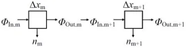
fluence from the first pixel,Φout, can then be calculated using Eq. (8) as shown in Fig.

4. The value of Φoutfrom the first pixel is set to equal Φinfor the second pixel and so

on. In this way, Eq. (6) can be used to calculate the number density as imaged by the second pixel. This procedure is continued to the last pixel-volume of the Na plume. The percentage of total IFT can be calculated by the difference between the total

14 increased by 0.01 iteratively until the final measured Φout equals the final calculated Φout.

The total amount of atomic Na (in percentage of black liquor solids, BLS) released is calculated from the integration of the mass flux, ΦNa, across the Na plume over time.

The mass flux is obtained from the area-based integral of atomic Na concentration,

nm, after correction for trapping, through the circular cross-section of the plume from xm to xc, multiplied by the mean gas velocity of the flame, Ū shown in Eq. (11). Here,

the gas velocity is calculated using the ideal gas law.

ΦNa,m = nm× (π ((xc– xm) 2 - (xc– xm+1)2) ) × Ū (11)

Similar procedures are repeated at incremental heights through the laser sheet to obtain the atomic Na concentration and the mass flux.

4. Results

A relationship between IFT and absorption, A was obtained from the previous

equations and the measured A for a range of excess oxygen (O2) concentrations in the

flame is shown in Fig. 5. Note that the range of O2 concentrations was 0–3.7%. It is

evident that IFT becomes significant only when A > 5%. The average of 25 successive

corrected images of the atomic Na plume during the smelt phase at t = 20–25 s is shown in Fig. 6. Note that Fig. 6 is the corrected image of Fig. 2 and the left-hand and right-hand sides of the corrected image were found to be symmetrical. It can be seen that the peak signal is about 0.9 ppm for Øb = 0.9 and 1.4 ppm for Øb = 1.25. The

15 found to be less than 1% of the laser radiation absorption by the atomic Na under fuel rich conditions. This was assessed by de-tuning the laser 1 nm off the D1 line.

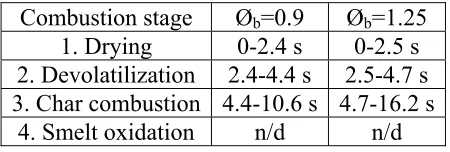
Table 2 presents the results of the analysis of the images obtained from the SLR camera, used to determine the duration of each stage of the black liquor combustion. The first three stages were easily detectable but the last stage of smelt oxidation, distinct by the intense glow of salt residue [4], could not be separated from the glow of the salt itself at the high temperatures in the flame. No significant influence of O2

concentration on the drying and devolatilisation time was observed for either condition. However, the time to complete the combustion of the char was 11.5 s (t = 4.4–16.2 s) for Øb = 1.25 compared with 6.2 s (t = 4.4–10.6 s) for Øb = 0.9 as shown

16 and liquid Na salts from the gaseous Na in the plume can be neglected. Hence, too, the use of polarising filters was found to be sufficient.

For Øb = 1.25, the concentration of atomic Napeaked at 1.5 ppm at the beginning of

the smelt phase (21 s) as shown in Fig. 7b. Under these conditions, the correction accounts for some 90% of the final value, with the uncorrected value being 0.16 ppm. For Øb = 0.9, the peak concentrations of atomic Na was 0.65 ppm at 15 s, a factor of

4.6 times the 0.14 ppm without the correction, as shown in Fig. 8b. Complete combustion for Øb = 1.25 and Øb = 0.9 occurs at approximately 240 and 550 s,

respectively. The duration of the combustion stage is about 2.5 times longer for Øb =

0.9 than for Øb = 1.25. The measured concentration of the atomic Na release during

the smelt phase of black liquor combustion is underestimated by at least an order of magnitude without correction, as is shown in Figs. 7 and 8. From the smelt analysis, no significant release of Na was detected for the first 20 s for both conditions, as is shown in Figs. 7b and 8b. Approximately 60% and 90% of Na is volatilised between

t = 20-160 s, during the smelt phase, for Øb = 0.9 and Øb = 1.25, respectively.

Practically, all of the Na has been released by 300 s for Øb = 0.9 and by 240 s for Øb =

1.25. Some atomic Na was still detected between t = 300–550 s even though the percentage of Na in the residue is almost zero at 300 s.

The concentration of the atomic Na was found to be constant with axial distance at a height of x/ro = 26, above the particle and sufficiently far from the particle surface to

17 velocity can be calculated from the ideal gas law. Within this region, the temperature and pressure are also approximately constant, and atomic Na can be expected to be close to equilibrium. The total amount of atomic Na released during char combustion was estimated by this approach to be 1.25 × 10-3 % for Øb = 0.9 and 2.54 × 10-3 % for

Øb = 1.25. These amounts are approximately half an order of magnitude higher than

that released during the drying and devolatilisation stages due to the longer duration of the char combustion stage (Table 2 and Fig. 9). The most significant release of atomic Na is found to occur during the smelt phase for both conditions. This accounts for approximately 99.9% of the total release of atomic Na for through all stages of combustion. The total atomic Na released for Øb = 1.25 was found to be 0.4%, which

is 50% higher than that for Øb = 0.9 as shown in Fig. 9 although the duration of the

combustion is about 2.5 times shorter for Øb = 1.25 than for Øb = 0.9.

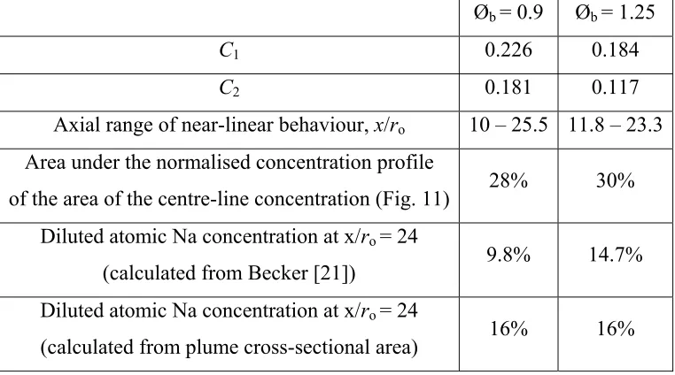
As described in Section 2, the dilution ratio was estimated assuming a jet, based on the analysis of Becker et al. [21]. For this estimate, the diameter of the nozzle was based on that of wire loop, i.e. 3 mm, so that ro = 1.5 mm and the measured atomic Na

concentrations for both stoichiometries were obtained during the smelt phase at the period of t = 20–40 s. The value of C1 for Øb = 0.9 and Øb = 1.25, respectively, was

obtained from the relationship between the normalised concentration half-radius, b1/2,

and the distance from the nozzle, x/ro. The value of C2 for Øb = 0.9 and Øb = 1.25,

18 The linear dependence of both Cref/C and b1/2/ro on x/ro within the “mixing region” of

the Na plume and the combustion products is shown for both stoichiometries in Fig. 10. Note that the plume temperature along the centre-line was approximately constant. Further evidence that the flow is self similar in the “mixing region” can be found in the normalised radial profiles of the mean concentration, C/Cc, shown in Fig. 11.

Theses profiles can be described by Eq. (12). By integrating the f (r/r1/2) of each of the

selected x/ro, the averaged area under the normalised concentration profile was

calculated to be 28% of the area of the centre-line concentration for Øb = 0.9 and 30%

for Øb = 1.25.

C/Cc= f (r/r1/2) (12)

The concentration of atomic Na diluted by the combustion products entrained into the Na plume can then be calculated x/ro = 26 from the inverse of Cref/C multiplied by the

averaged area under the normalised concentration profile. The comparison of these estimates of the diluted atomic Na concentration with those calculated from the cross-sectional area of the Na plume divided by that of the burner for both stoichiometries is presented in Table 3. The two methods agree for Øb = 1.25. However, for Øb = 0.9,

the diluted atomic Na concentration calculated from the Na plume cross-sectional area is almost 40% below the similarity value as shown in Table 3.

At a height of x/ro = 26 above the particle, it was found that Cref/C = 2.82 and 2.1 for

Øb = 0.9 and Øb = 1.25, respectively. These values correspond to 35% and 48% of the

concentration of atomic Na being diluted by 65% and 52% of the combustion products for Øb = 0.9 and Øb = 1.25, respectively. The average of the measured

atomic Na concentrations for Øb = 0.9 at the exposure time of t = 20–40 s, 40–100 s,

19 ppm, respectively, while that of the calculated Na concentrations was found to be 0.86, 0.33, 0.56, and 0.133 ppm, respectively. For Øb = 1.25, the average of the

measured atomic Na concentrations at the exposure time of t = 20–40 s, 40–80 s and 80–120 s at the centre-line was found to be 0.58, 0.63 and 0.65 ppm, respectively, while that of the calculated Na concentrations was found to be 1.9, 3.4 and 2.7 ppm, respectively, as shown in Fig. 12. Note that the calculated distribution of the Na at equilibrium using the PFR model agreed well with the SER model. The models were found to over-estimate the average of the atomic Na concentrations by a factor of 1.7 for Øb = 0.9, and a factor of 3.3 for Øb = 1.25 as shown in Fig. 12. The range of

results calculated from model for both stoichiometries had an estimated rms of

±40%, based on the input Na from the smelt analysis at the different exposure times. The error bars on the measured atomic Na concentrations for both stoichiometries were found to be approximately ±25% and details of the uncertainties are described in Section 5. Hence the model and experiments agree within experimental uncertainty for Øb = 0.9 and within a factor of about 2 for Øb = 1.25.

The major Na species in the gas-phase are calculated using the PFR model to be Na and NaOH during the smelt phase at t = 20–40 s for both stoichiometries, as shown in Fig. 13. Note that the distribution between gaseous Na and NaOH is equivalence ratio dependence and the kinetic reactions reach equilibrium within 15 ms. Other Na species identified in both the models were NaO, NaO2 and NaSH. However, only

volume concentrations above 0.0001 ppm are as shown in Fig. 13. The calculated concentration of Na for Øm = 1.25 is approximately 3.5 times higher than that for Øm

20 measurements during the smelt phase at t = 20–40 s, when differences between Øm

and Øb are small.

5. Discussion

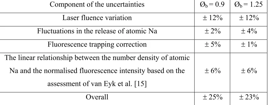
The effect of collisional quenching on the fluorescence signal is accounted for in the information from the measured absorption, which is not affected by the quenching. The fluctuation between the points shown in Figs. 7 and 8 is primarily due to the inconsistency of the laser power, although a laser measurement correction method for these variations has been applied. The rms in the scatter of the corrected INa was

calculated to be about ±25% for Øb = 0.9 and ±23% for Øb = 1.25. This accounts for

the variation in the laser fluence, fluctuations in the release of atomic Na from the burning black liquor droplet, the fluorescence trapping correction and uncertainties in the linear relationship between the number density of atomic Na and the normalised fluorescence intensity based on the assessment of van Eyk et al. [15] for their coals as shown in Table 4.

The average of the atomic Na concentrations measured with PLIF were found to underestimate it by a factor of 2.0 for Øb = 0.9, and a factor of 4.5 for Øb = 1.25.

21 errors from the mixing model and equilibrium calculation caused by the uncertainties of the PLIF measurement and flame temperature, respectively. Note that the mixing model has less uncertainty than the quantitative PLIF because it only depends on the half-width and centre-line decays. Therefore, this does not need the absolute correction.

That the major Na species calculated with the model are NaOH and Na for both conditions agree with previous studies [9–11]. The study by Schofield and Steinberg [25] has shown the significance of sulphur on the Na–S chemistry under fuel rich conditions, with the S/Na ratio of at least 5 orders of magnitude greater. However, no significant influence of sulphur on the Na–S chemistry is found in the present study due to the S/Na ratio being approximately an order of magnitude smaller. Most of the sulphur content was calculated to be converted to SO2 rather than Na–S species for

both conditions.

The average measured total flux of atomic Na for Øb = 1.25 was found to be 1.5 times

that for Øb = 0.9, while the average calculated ratio was approximately 5. The main

reasons for this difference are expected to derive from the assumption in the model that the gases are well mixed, while significant gradients are clearly present in the real plume. In addition, the mass flux of the atomic Na is also dependent on the area of the plume, as shown in Eq. (9).

22 Na is released during the drying, devolatilisation and char combustion stages compared with that during the smelt phase.

6. Conclusions

A quantitative measurement of high atomic Na concentration release of a burning black liquor droplet with a method to correct for the fluorescence trapping IFT has

been demonstrated. The overall accuracy of this method is estimated to be approximately ±25% for Øb = 0.9 and ±23% for Øb = 1.25. Nevertheless, the high

concentration of atomic Na during smelt phase results in the size of the correction being about 90% of the final value, justifying an independent assessment. The independent assessment was performed using equilibrium calculations based on the estimated dilution of plume gases with gas combustion gases, and measured mass losses from the particle obtained separately, via rapid cooling. This was found to give reasonable agreement with LIF for Øb = 0.9, but to under estimate by a factor of four

for Øb = 1.25. Importantly, the independent values are higher than the PLIF values,

confirming that the correction, while large, is not over estimated.

The key findings of these assessments are:

(i) the incorporation of a correction for fluorescence trapping allows reliable measurement of the distribution of atomic Na by PLIF at concentrations of 1 ppm, as can occur during black liquor combustion;

23 (iii) the total mass flux of atomic Na during the combined stages of drying, devolatilisation and char combustion stages is very small, at 0.003% of black liquor solids for the present conditions, and two orders of magnitude less than the 0.3% in smelt phase; and

(iv) both the concentration and mass flux of atomic Na exhibit a relatively weak dependence on the stoichiometry of the burner gases, being no more than about 60% higher for Øb = 1.25 than for Øb = 0.9 under the present conditions. This is

significantly less than predicted by the models.

7. Acknowledgements

The authors would like to acknowledge Mr Philip van Eyk, Centre of Energy Technology (CET) who assisted in the experimental setup and data analysis. Dr Paul Medwell, CET, also assisted with the data analysis.The project has been undertaken as part of a broader collaboration with Prof Mikko Hupa and Mr Mikael Forssén of the Process Chemistry Centre, Åbo Akademi University. They contributed to the planning and interpretation of the overall research program and provided the black liquor samples used in the present investigation. The anonymous reviewers of the paper are also gratefully acknowledged for their insight comments on the paper.

8. References

[1] T. N. Adams, J. M. Frederick, T. M. Grace, M. Hupa, K, Iisa, A. K. Jones, H. Tran, Kraft Recovery Boilers, Tappi Press, 1997, p. 3.

24 Methanol/DME Production as Motor Fuels for Automotive Uses, Altenar II Report, Contract No. XVII/4.1030/Z/01-087/2001, Dec 2003.

[3] R. A. Wessel and L. L. Baxter, TAPPI J. 2 (2003) 19-24.

[4] M. Hupa, P. Solin and R. Hyöty, J. Pulp Paper Sci. 13 (1987) 67-72. [5] J. Li and A. R. P. van Heiningen, TAPPI J. 73 (1990) 213-219. [6] J.H. Cameron, J. Pulp Paper Sci. 14 (1988) 76-81.

[7] E. I. Kauppinen, M. P. Mikkanen, T. Valmari, S. A. Sinquefield, W. J. Frederick, M. Hupa, R. Backman, M. Forssén, P. McKeough, V. Arpiainen, M. Kurkela, M. Moisio, J. Keskinen, and M. Mäkinen, Sodium Release during Black Liquor Pyrolysis: Differences Between the Results from Various Laboratory Scale Experiments, Proc. 1995 Int’l Recovery Conf., Toronto, p. 105-112.

[8] C. L. Verrill, T. M. Grace and K. M. Nichols, J. Pulp Paper Sci. 20 (1994) 354-360.

[9] L. Pejryd and M. Hupa, Bed and Furnace Gas Composition in Recovery Boilers – Advanced Equilibrium Calculations, 1984 TAPPI Pulping Conference, San Francisco, p. 579-590.

[10] A. Borg, A. Teder, and B. Warnqvist, TAPPI J. 57 (1974) 126-129.

[11] W. L. Saw, M. Hupa, P. J. Ashman, G. J. Nathan, M. Forssén, and Z. T. Alwahabi, Insight into the Fate of Atomic Sodium from Black Liquor Combustion in a Flat Flame using Equilibrium Calculations, Proc. Australian Combust. Inst. 2007, p. 118-121.

[12] J. W. Daily and C. Chan, Combust. Flame 33 (1978) 47-53.

25 [14] W. L. Saw, G. J. Nathan, P. J. Ashman, Z. T. Alwahabi, M. Forssén and M. Hupa, Assessment of the release of sodium from a burning black liquor droplet using Planar Laser-Induced Fluorescence (PLIF) and smelt analysis, Int’l Chemical Recovery Conf., Tappi Proc. 2007, p. 97-100.

[15] P. J. van Eyk, P. J. Ashman, Z. T. Alwahabi, G. J. Nathan, Combust. Flame 155 (2008) 529-537.

[16] J. W. Daily, Appl Opt. 17 (1978) 1610-1615.

[17] K.T. Hartinger, S. Nord, P.B. Monkhouse, Appl. Phys. B 64 (1997) 363-367. [18] M. Y. Choi and K. A. Jensen, Combust. Flame 112 (1998) 485-491.

[19] P.J. van Eyk, P.J. Ashman, Z.T. Alwahabi and G.J. Nathan, Proc. Combust. Inst. 32 (2009) 2099-2106.

[20] R. M. Fristrom and A. A. Westenberg, Flame Structure, McGraw-Hill, 1965. [21] H. A. Becker, H. C. Hottel and G. C. Williams, J. Fluid Mech. 30 (1967) 303.

[22] G. P. Smith, D.M. Golden, M. Frenklach, N.W. Morinarty, B. Eiteneer, M. Goldenberg, C.T. Bowman, R.K. Hanson, S. Song, W.C. Gardiner Jr., V.V. Lissianski, and Z. Qin, http://www.me. berkeley.edu/gri_mech/.

[23] P. Glarborg, and P. Marshall, Combust. Flame 141 (2005) 22-39.

[24] M. U. Alzueta, R. Bilbao and P. Glarborg, Combust. Flame 127 (2001) 2251.

26 Table 1

The elemental composition of the black liquor, given as percent of dry solid content

Element % Carbon 30.3

Hydrogen 3.5 Nitrogen 0.2

27 Table 2

Typical duration of each combustion stage

Combustion stage Øb=0.9 Øb=1.25

1. Drying 0-2.4 s 0-2.5 s 2. Devolatilization 2.4-4.4 s 2.5-4.7 s 3. Char combustion 4.4-10.6 s 4.7-16.2 s

4. Smelt oxidation n/d n/d

28 Table 3

Estimation of the diluted atomic Na concentration for Øb = 0.9 and Øb = 1.25

Øb = 0.9 Øb = 1.25

C1 0.226 0.184

C2 0.181 0.117

Axial range of near-linear behaviour, x/ro 10 – 25.5 11.8 – 23.3

Area under the normalised concentration profile

of the area of the centre-line concentration (Fig. 11) 28% 30% Diluted atomic Na concentration at x/ro = 24

(calculated from Becker [21]) 9.8% 14.7%

Diluted atomic Na concentration at x/ro = 24

29 Table 4

The component of the uncertainties of the INa for Øb = 0.9 and Øb = 1.25

Component of the uncertainties Øb = 0.9 Øb = 1.25

Laser fluence variation ±12% ±12%

Fluctuations in the release of atomic Na ±2% ±4% Fluorescence trapping correction ±5% ±1% The linear relationship between the number density of atomic

Na and the normalised fluorescence intensity based on the assessment of van Eyk et al. [15]

±6% ±6%

30 FIGURE CAPTIONS

Figure 1: The experimental apparatus used to image atomic Na by PLIF and also absorption, during the combustion of a black liquor droplet.

Figure 2: Raw image of the atomic Na PLIF signal from the plume and from the two dye cells, from which the laser sheet profile and absorption can be obtained. [Note: au = arbitrary units]

Figure 3: Schematic diagram of the effects of absorption and fluorescence trapping,

IFT.

Figure 4: Schematic diagram of IFT correction on each pixel.

Figure 5: The variation of Fluorescence Trapping, IFT with Absorption, A.

Figure 6: The average of 25 successive two-dimensional images of the concentration of atomic Na during the smelt phase at t = 20-40 s for a) Øb = 0.9 and; b) Øb = 1.25.

Figure 7: The concentration of atomic Na in the plume of a droplet of black liquor during each stage of combustion with (□) and without (∆) the trapping correction for Øb = 1.25 at a) t = 0–20 s; and b) t = 0–300 s and the mass fraction of Na left in the

31 Figure 8: The concentration of atomic Na in the plume of a droplet of black liquor during each stage of combustion with (□) and without (∆) the trapping correction for Øb = 0.9 at a) t = 0–20 s; and b) t = 0–600 s and the mass fraction of Na left in the

residue over time. The stages marked as ‘1’ to ‘4’ are identified in Table 2.

Figure 9: Total atomic Na released during the drying, devolatilization, char combustion and smelt phase stages at equilibrium at a height of x/ro = 26.

Figure 10: The normalised concentration half-radius, and the reciprocal of the normalised centre-line mean concentration, as a function of distance from the nozzle for Øb = 0.9 and 1.25.

Figure 11: The normalised radial profiles of the mean concentration, C/Cc, within the

near-linear mixing region a) Øb = 0.9 and b) Øb = 1.25.

Figure 12: Comparison of the average of the measured atomic Na concentrations using PLIF, with the calculations based on equilibrium of measured residue and the respective Cref/C, at different exposure time for a) Øb = 0.9 (experiment), Øm = 0.9

(model) and b) Øb = 1.25, Øm = 1.25.

Figure 13: The distributions of the major Na species based on equilibrium of measured residue and the respective Cref /C at t = 20–40 s as a function of residence

33 r (mm)

X (mm)

−40

−50 −30−20−10 0 10 20 30 40 50

45

35

25

15

2000 4000 6000 8000

Relatitve Intensity (au)

36

0 10 20 30 40

0 5 10 15 20 25 30

Fluorescence Trapping,

Ft

(%)

Absorption, A

I

37 r

X

(mm)

10

−20 −10 0 20

45

35

25

15

0.2 0.4 0.6 0.8

(mm)

[Na] (ppm)

a)

38 r

X

(mm)

−20 −10 0 10 20

45

35

25

15

0.2 0.4 0.6 0.8 1 1.2 1.4

(mm)

[Na] (ppm)

b)

39

with correction without correction Na in residue

0 5 10 15 20

0 0.1 0.2 0.3 0.4 0.5

Time (s)

[Na](ppm)

1 2 3 4

a)

40

0 50 100 150 200 250 300

0 0.5 1 1.5 2

Time (s)

[Na](ppm)

with correction without correction Na in residue

0 20 40 60 80 100

Na in residue (% of Na in BLS)

b)

41

0 5 10 15 20

0 0.1 0.2 0.3 0.4 0.5

[Na] (ppm)

Time (s)

1 2 3 4

a)

42

0 100 200 300 400 500 600

0 0.2 0.4 0.6 0.8 1

[Na](ppm)

Time (s)

with correction without correction Na in residue

0 20 40 60 80 100

Na in residue (% of Na in BLS)

b)

43

10−4 10−3 10−2 10−1 100

Total atomic Na release (% of BLS)

Ø

b = 0.9

Ø

b = 1.25

Drying Devol. Char

Combustion Smelt

44

5 10 15 20 25 30 35

0 1 2 3 4

C ref

/C

x/r

o

Ø

b = 0.9

Ø

b = 1.25

Equilibrium Mixing

a)

45

5 10 15 20 25 30 35

1 2 3 4 5 6 7

b 1/2

/r

o

x/r

o

Ø

b = 0.9

Ø

b = 1.25 Mixing

Equilibrium

b)

46

0 1 2 3 4

0 0.2 0.4 0.6 0.8 1

C/C

c

r/r

1/2

x/r

o = 10.0

x/r

o = 13.3

x/r

o = 16.7

x/r

o = 20.0

x/r

o = 23.3

a)

Figure 11

47

0 1 2 3 4

0 0.2 0.4 0.6 0.8 1

C/C

c

r/r

1/2

x/r

o = 13.3

x/r

o = 16.7

x/r

o = 20.0

x/r

o = 23.3

b)

48

0 0.2 0.4 0.6 0.8 1 1.2 1.4

[Na](ppm)

PFR and SER Models PLIF Measurement

t = 20−40st = 40−100s t = 100−200st = 200−300s

a)

49

0 1 2 3 4 5 6

[Na](ppm)

PFR and SER Models PLIF Measurement

t = 20−40 s t = 40−80 s t = 80−120 s

b)

50

10−4 10−3 10−2 10−1 100 101

[Na](ppm)

Ø

m = 0.9

Ø

m = 1.25

NaOH Na NaO NaO

2 NaSH