Average cosmic evolution in a lumpy universe

(1)

Department of Physics and Astronomy University of Canterbury, Private Bag 4800

Christchurch, New Zealand

PHYS 690 MSc Thesis

submitted in partial fulfilment of the requirements for

The Degree of Master of Science in

Physics

Average cosmic evolution

in a lumpy universe

by

James A.G.

_Duley

Supervisor:

Assoc. Prof. David L.

_Wiltshire

Assistant Supervisor:

Dr Teppo

Mattsson

(2)

(3)

To my parents, who without their help and encouragement I would not

(4)

(5)

Acknowledgements

Firstly, I would like to acknowledge my supervisor, David Wiltshire, for his help and guidance of this thesis. Secondly, I would like to acknowledge the following people for their proofreading efforts; Teppo Mattsson, Josephine Faulkner, Alice Balme, Ahsan Nazer and Michael Pitman.

(8)

(9)

Abstract

The procedure of averaging and coarse-graining of the gravita-tional field equations with sources are investigated in both Newto-nian gravity and in general relativity. In particular the schemes of Buchert and Korzy´nski are examined and compared in both situa-tions. In Newtonian gravity it is shown how to calculate the tidal tensor given boundary conditions for it and how to average it given those boundary conditions. It is also shown that one can always choose boundary conditions to make the average tidal tensor vanish or take any value.

The problems of coarse-graining tensors in general relativity are critically examined, and a set of relevant conditions for such a pro-cedure are enumerated. Korzy´nski’s covariant coarse-graining pro-cedure is reviewed and applied to a particular case. For the case of the Lemaˆıtre-Tolman-Bondi model it is shown that the backreaction was always zero for a centred spherical coarse-graining domain.

Wiltshire’s timescape model, which applies a particular obser-vational interpretation to Buchert’s averaging scheme, is reviewed. The dust timescape model of Wiltshire is extended by the addition of a homogeneous radiation source. This model is solved numerically and it is shown not to vary significantly from the dust model since the redshift z _≈ 30, which is when the backreaction and radiation density are equal. The model is integrated back in time from the sur-face of last scattering with results indicating a breakdown in aspects of the model at early times.

(10)

(11)

Conventions

Unless otherwise noted, the following conventions will be used. Units will be used such that c = 1. In reference to spacetime, Greek indices will be taken to be 0,1,2,3 and Latin indices will be taken to be 1,2,3; the first half (a to g) will be used to denote Euclidean space and the middle letters (i to p) to denote the spatial indices of a 3+1 split of spacetime. In reference to coarse-graining on an arbitrary dimensional manifold, Greek indices will indicate a coordinate basis and Latin indices will indicate a non-coordinate basis. Einstein summation convention shall be assumed. Tensor signs will follow that of Misner, Thorne and Wheeler [1], i.e.,

M etric signature: ηµν = diag(−1,+1,+1,+1) (1)

Riemann tensor: Rµ_ναβ =∂αΓµνβ−∂βΓµνα+ ΓµσαΓσνβ −ΓµσβΓσνα (2)

Einstein tensor : Gµν ≡Rµν− 1₂gµνR= 8πGTµν (3)

A comma shall denote a partial derivative, whereas a semicolon will denote a covariant derivative, i.e., Xβ_,α ≡ ∂αXβ and Xβ;α ≡ ∇αXβ. Parentheses

around indices shall denote symmetrization on those indices, i.e.,

A_···(α1···αp)···≡

1

p!

X

σ∈Sp

A_···(ασ(1)···ασ(p))···, (4)

(12)

xii Conventions

for permutations σ. Square brackets around indices shall denote antisym-metrization on those indices, i.e.,

A_···[α1···αp]···≡

1

p!

X

σ∈Sp

sgn(σ)A_···[ασ(1)···ασ(p)]···, (5)

where sgn(σ) is the sign of the permutation σ. The Levi-Civita symbol is defined as

α1α2···αn =

      

+1 ifα1α2· · ·αn is an even permutation of the index range

−1 ifα1α2· · ·αn is an odd permutation of the index range

0 otherwise

(6) and the Levi-Civita pseudotensor as

ηµνσρ =

q

−det(gµν)µνσρ. (7)

Also, we will define the following tensor derived from the metric,

(13)

CHAPTER

1

Introduction

1.1 Inhomogeneous cosmology

The assumption that the universe is homogeneous and isotropic was cer-tainly very accurate at the time of last scattering, evident from the near perfectly smooth cosmic microwave background (CMB). During the inter-vening aeons formation of large scale structures has led to a universe that is no longer near to homogeneous, but rather dominated by voids with galaxy clusters in filaments and walls threading and surrounding these voids. This is seen in sky surveys such as the Sloan Digital Sky Survey (SDSS) [2], 2dF Galaxy Redshift Survey and others. These surveys show that voids with a characteristic mean effective radii of order (15 ±3)h−1 _Mpc1 _and a typical density contrast of δρ/ρ = −0.94±0.02, where ρ is the average density of the observed volume, compose 40% of the volume of the nearby universe [3, 4]. A study [5] of the Sloan Digital Data Release 7 [6] found the median effective radius of voids in the survey volume of 17h−1 _{Mpc and} 62% of the volume is occupied by voids with mean effective radii between 10h−1 _{Mpc and 30}_h−1 _{Mpc. Along with voids of this size there an} abun-dant amount of smaller voids occupying the universe [7] meaning overall

1_{Due to the ellipticity some voids exhibit, the mean effective radius is defined as the}

radius of a sphere occupying the same volume.

(14)

2 Introduction

the current universe is dominated by voids.

The non-linear nature of the Einstein equations makes trying to solve them for the full inhomogeneous geometry of the universe extremely difficult to do analytically with today’s current mathematical knowledge, or even numerically with today’s computing power. The difficulties in numerical relativity go beyond the simple limits imposed by hardware limitations. To solve Einstein’s equations requires a splitting of spacetime into space and time in order to construct evolution equations. Such a splitting involves intrinsic ambiguities. Further problems arise when structures form and geodesics cross. Any numerical scheme has to deal with smoothing over singularities. In cosmology, in view of the complex hierarchy of observed structure, we have the additional problems of coarse-graining over these structures to define average symmetries of the global spacetime background.

The simplifying assumptions most cosmologists make is that, firstly, the

universe is on average homogeneous and isotropic and, secondly, on

aver-age it evolves like an exactly homogeneous isotropic Friedmann-Lemaˆıtre-Robertson-Walker (FLRW) model. The first assumption seems to be valid on scales of over 100h−1_{Mpc, although there is some debate as what exactly} this scale is [8, 9]. The second assumption concerning average evolution, however, has no direct physical justification. A further third assumption that is also often made is that our own measurements yield parameters which exactly coincide with those that describe the average cosmic evo-lution (which means those of a FLRW model if we also make the second assumption).

(15)

1.1. Inhomogeneous cosmology 3

then match the geometry of the Milky Way to that of the local group, and so on until we have matched geometries up to the scale which describes the average cosmic evolution and propagation of light. There are several possible relevant steps of coarse-graining in this hierarchical process, with qualitatively new physical questions entering when we make a transition from dealing with bound systems to regions of expanding cosmic fluid [12]. If we ignore the fitting problem and make the standard assumptions con-cerning homogeneity and isotropy then current cosmological observations indicate that the expansion rate of the universe appears to have begun accelerating in the relatively recent past, at redshifts z <1. Given the in-trinsically attractive nature of gravity, an acceleration of cosmic expansion is not possible if the universe contains only sources of mass–energy which obey the strong energy or “timelike convergence” condition, which for per-fect fluids is characterized by an equation of state for which p >−1

3ρ. The strong energy condition must be satisfied in order for matter to focus light rays, and it is satisfied for all forms of matter which have been directly observed.

A form of matter which violates the strong energy condition is therefore required, and observationally the equation of state of such a fluid which best fits cosmological observations is found to be extremely close to the lowest possible bound, p=₋ρ, allowed by the dominant energy condition2_. The p=−ρbound is realised by a cosmological constant, which represents a pure vacuum energy. Generically any form of matter which violates the strong energy condition will not clump as a result of gravitational collapse, and is therefore called dark energy. Dark energy is, as of yet, not directly observed and its only manifestation is to change the expansion history of the universe to allow for cosmic acceleration.

Since the determination of the average expansion history of the universe is intimately related to the assumptions of homogeneity and isotropy in the

2_{Physically, the dominant energy condition,} _|_p_{| ≤} _ρ_{, may be understood as saying}

(16)

4 Introduction

standard ΛCDM model, it is possible that the expansion history has been misinterpreted as a result of incorrect assumptions in a complex geometrical problem. This thesis will investigate what happens if we do not make such assumptions.

To perform such a task we need to first decide what is meant by an average. The concept of an average in general relativity is not a trivial one. We will present and analyse two methods that define the concept of an average, those of Korzy´nski [13] and of Buchert [14, 15]. These show that the Einstein equations of the average geometry and the average of the Einstein equations of the full geometry are not the same; the difference leads to abackreaction term. We will then generalise Wiltshire’s timescape model [16] to include radiation. The timescape model drops the second and third assumption above and, after a particular physical interpretation of our own measurements relative to both cosmic averages and cosmic variance, fits observed data well without dark energy.

1.2 Thesis outline

Before beginning our discussions on averaging in general relativity, we will look at the simpler case of averaging in Newtonian cosmology first. This is presented in Chapter 2 where we start by reviewing the existing formulation of Newtonian gravity and proceed to averaging while deriving some new results along the way.

In Chapter 3 we review the kinematical description of spacetime and compare that with Newtonian gravity. We then review the 3+1 split of spacetime and some useful coordinate systems. This is followed by a review of hypersurfaces and then the Arnowitt-Deser-Misner (ADM) gauge [17, 18, 19].

(17)

1.2. Thesis outline 5

the velocity gradient and apply it to the Bianchi I universe. Following Korzy´nski, we then develop the evolution equation for the coarse-grained velocity gradient and then apply the procedure to the Lemaˆıtre-Tolman-Bondi model.

In Chapter 5 we begin by reviewing the Buchert averaging formalism for dust. We then describe the timescape model and apply the Buchert aver-aging formalism and then describe how observables are related to variables of the timescape equations. Following this we proceed by adding homoge-neous radiation to the model and analysing the results. Next we attempt to solve the model beyond the surface of last scattering and discuss the prob-lems of doing so. This is followed by a discussion on the initial conditions and the merits of combining the timescape model without radiation with a homogeneous model with radiation at an earlier time.

(18)

(19)

CHAPTER

2

Newtonian cosmology

2.1 Introduction

The approach we will adopt in this chapter predominantly follows the inves-tigations of Buchert and Ehlers in 1997 [14] and by Korzyński in 2010 [13], supplemented by that of Zalaletdinov who wrote a rigorous series of papers on the subject in 2002 [20, 21, 22]. The work of Buchert and Ehlers was the first published work on the subject of averaging Newtonian cosmology and led to Buchert’s extension of the scheme to general relativity [15, 23]. Whereas Buchert and Ehlers looked at differences relative to a homoge-neous and isotropic cosmology, Korzyński generalised it to looking at the differences relative to just a homogeneous cosmology. This is preparation for Korzyński’s method of coarse-graining in general relativity, which is the main subject of the same paper [13].

2.2 Governing equations

Consider a pressureless fluid, henceforth referred to by the term dust, in Euclidean space E3, interacting under the influence of Newtonian gravity. This system is described in Cartesian coordinates, xa_{, by the local}

den-sity function ρ(xa_{, t}_{), velocity field} _va _xb_{, t} _{and the Newtonian potential}

(20)

8 Newtonian cosmology

φ(xa_{, t}_{). The evolution of this system is governed by the following system}

of PDEs known as theEuler-Poisson equations,

∂va

∂t +v

b∂va

∂xb =−δ ab ∂φ

∂xb (2.1)

∂ρ ∂t +v

b ∂ρ

∂xb =−ρ

∂va

∂xa (2.2)

δab ∂

2_φ

∂xa_∂xb = 4πGρ. (2.3)

Following Buchert and Ehlers [14], we can define the gravitational acceler-ation by

ga =−δab∂φ

∂xb (2.4)

and rewrite equations (2.1)-(2.3) in terms ofg. Rewriting the LHS of (2.3) as the negative divergence of the gravitational acceleration, _{−∇ ·}g, with the addition of a fourth equation requiring the gravitational acceleration be a conservative field,∇ ×g= 0, yields the desired result. We will, however, leave the equations in terms of the gravitational potential.

The position of a dust particle can be given in Eulerian coordinates by xa ₌ _fa _Xb_{, t}_{, where} _Xb _{denotes the Lagrangian coordinate of the}

dust particle which is constant with respect to any given dust particle. We define the total time derivative, d

dt, as the time derivative with respect to a

dust particle, i.e., at fixed Xa_, d

dt ≡ (. . .)˙ = ∂

∂t in Lagrangian coordinates.

The velocity field is then va ₌ dxa

dt = ∂

∂tfa and the total time derivative

in Eulerian coordinates is _dd_t ≡ (. . .)˙ = _∂t∂ +vb ∂

∂xb. The left-hand side of

equations (2.1) and (2.2) can then be realised to be ˙va _{and ˙}_ρ _{respectively.}

Equations (2.1)-(2.3) are invariant under the kinematical group of trans-formations,

xa→xa0 =Aabxb +Da(t) t →t0 =t+b (2.5)

whereAa

b is a constant real-valued orthogonal matrix and Da(t) is an

arbi-trary function of time. Under this change of coordinates, the gravitational potential, φ(xa_{, t}_{), undergoes the following transformation,}

φ_→φ0 =φ₋δab

d2_Da₍_t₎

dt2 x

(21)

2.2. Governing equations 9

Zalaletinov [21] gives this group of transformations but erroneously scales

t by a constant factor a and does not require Aa

b to be orthogonal. The

consequence of the invariance under this group of transformations is that inertial observers cannot be defined as the lack of invariance of the inertial and gravitational acceleration, dva

dt and g

a _{respectively, means that it is}

impossible to distinguish between the two. We cannot say if the inertial acceleration, d_dv_ta, is zero which is what defines an inertial observer.

The reason for the undefined inertial frames is a result of the ill-posedness of equations (2.1)-(2.3) when only supplemented with initial conditions and

not boundary conditions. Poisson’s equation (2.3) does not have a unique

solution unless we can place boundary conditions on φ, which in

study-ing the infinite Newtonian cosmology we generally cannot. It is only when

boundary conditions are placed on φ that it becomes uniquely defined and

d2_Da

dt2 must be zero. This results in the kinematical group of transformations

reducing to the Galilean group of transformations,

xa→xa0 =Aa_bxb +Bat+Ca t→t0 =t+b, (2.7)

where Aa

b is a constant real-valued orthogonal matrix and Ba and Ca are

constants also. An example of such a case [21] is when we have an isolated fluid, and we demand the global boundary condition of vanishing potential at infinity,

φ(xa, t)→0 as (xaxa) 1

2 → ∞. (2.8)

The ill-posedness is more evident with a more useful form of (2.1), ob-tained by taking a spatial partial derivative, so that (2.1)-(2.3) become

(va_,b)˙ =−va_,cvc_,b−φ,a_,b (2.9)

˙

ρ=−ρva_,a (2.10)

φ,a_,a = 4πGρ. (2.11)

(22)

σab, and the antisymmetric part or vorticity tensor,ωab,

va,b= 1₃θδab+σab+ωab, (2.12)

where

θ =va_,a =∇ ·v, (2.13)

σab =v(a,b)− 1₃θδab, (2.14)

and

ωab =v[a,b] =δ_[_acδ_b_]dvc,d = 1₂eabecdvc,d =−1₂eabζe, (2.15)

letting ζ = ∇ ×v be the curl of the velocity field. We can also perform a similar decomposition onφ,ab,

Θ =φ,a_,a = ∆φ (2.16)

Eab =φ,ab− 1₃Θδab, (2.17)

whereEab is referred to as the tidal tensor.

With the use of (2.13)-(2.17), equations (2.9)-(2.11) give, through some derivation, the transport equations,

˙

θ =−1 3θ

2₋_σ2₊_ω2₋_Θ _(2.18)

˙

σab =−2₃θσab−σacσcb −ωacωcb+13δab σ 2

−ω2₋Eab (2.19)

˙

ωab =−2₃θωab−σacωcb−ωacσcb or ζ˙ =−23θζ+ ¯σζ (2.20) ˙

ρ=ρθ (2.21)

Θ = 4πGρ, (2.22)

where the scalar shear and vorticity are, σ2 ₌ _σ

abσab and ω2 = ωabωab

respectively, and ¯σ denotes the matrix composed of the elements σab. We

see that we have a system of ODEs governing the evolution of all of the above variables except the tidal tensor, Eab. This can only be determined

through boundary conditions placed on φ, as opposed to the trace, which

(23)

We note the following integrability conditions on account of θ, σab, ωab

and Eab being derivatives,

1

3δa[bθ,c]+σa[b,c]+ωa[b,c]= 0, (2.23)

E_{a ,b}b = 8πG

3 ρ,a (2.24)

and

Ea[b,c] =− 4πG

3 δa[bρ,c]. (2.25)

We can place boundary conditions on Eab by specifying Eab on the

boundary, ∂Gt, of some domain Gt. These boundary conditions are not

completely arbitrarily specifiable, however, one must ensure they satisfy the integrability conditions (2.24) and (2.25) on ∂Gt, as well as obviously

being traceless and symmetric. Then one can solve forEab overGtby using

equations (2.24) and (2.25). This is performed using Helmholtz’s theorem, treating Eab as three separate vector fields labelled by a, Ea. Equations

(2.24) and (2.25) are then effectively the divergence and curl of Ea

respec-tively. Helmholtz’s theorem combined with

Z

Gt ∂A ∂xa d

3_x₌Z

∂Gt

A nadσ, (2.26)

which is a form of Stokes’ theorem, then leads to

Eab(xe, t) =Ba,b(xe, t) +bcdAac,d(xe, t), (2.27)

where

Ba(xe, t) =

1 4π

Z

∂Gt E g

a (x0f, t)− 8πG3 ρ(x0

f_{, t}₎_δ g a

p

(xe₋_x0e₎₍_x

e−x0e)

ng(x0f, t) dσ0 (2.28)

and

A_ac(xe, t) = 1 4π

Z

∂Gt

hcg Eah(x

0f_{, t}_{) +} 4πG

3 ρ(x0f, t)δah

p

(xe₋_x0e₎₍_x

e−x0e)

ng(x0f, t) dσ0. (2.29)

Here na is the outward pointing unit normal on ∂Gt. We can combine

(24)

integrals. However, the form does not become any more transparent, so we will not do so here.

The system will then have a unique solution up to the kinematical group of transformations (2.5) on theGt. An example of such a case is the general

Heckmann-Sch¨ucking boundary condition [24, 25],

Eab(xa, t)→E˚ab(t) as (xaxa) 1

2 → ∞, (2.30)

where ˚Eab(t) is some arbitrary function of t. By virtue of the integrability

conditions, (2.24) and (2.25), this boundary condition is only valid if

ρ(xa, t)→˚ρ(t) as (xaxa) 1

2 → ∞, (2.31)

where ˚ρ(t) is some function of t.

Alternatively, one could give an evolution equation for Eab which must

propagate the integrability conditions. This would then indirectly give

boundary conditions for Eab. An example of such an equation is given

by Bertschinger and Hamilton [26], the local tidal approximation,

˙

Eab =−θEab−δabσcdEcd+ 3σc(aEb)c+ωc(aEb)c−Θσab. (2.32)

At this stage, it is unclear to me whether (2.32) preserves the integrability conditions.

Solving the system

To solve the system we will assume that an evolution equation for Eab

has been specified, otherwise if boundary conditions are given explicitly equation (2.27) will couple all the equations making the following solution not just involve ODEs. Begin by solving the ODEs (2.18)-(2.22) and an evolution equation forEab from initial conditions

θ(Xa, t0) =θ0(Xa) ωab(Xc, t0) = ωab0(Xc) σab(Xc, t0) = σab0(Xc)

(25)

to give

va,b(Xc, t) (2.34)

by equation (2.12). Compared to solving (2.1)-(2.3), where one can give a completely arbitrary initial velocity profile, va₍_xb_{, t}

0), and density

pro-file, ρ(xa_{, t}

0), one must make sure (2.33) satisfy the integrability conditions

(2.23)-(2.25). If one derives (2.33) from an arbitrary initial velocity profile and density profile, the integrability conditions are, of course, trivially sat-isfied. Because (2.33) are given in Lagrangian coordinates, one would need to use the inverse of the Eulerian-Lagrangian transformation (fa

0 below) to check this, alternatively one could give (2.33) in Eulerian coordinates and change to Lagrangian coordinates to do the solving. One can then show that

∂ ∂t

∂fa

∂Xb

=va_,c ∂f

c

∂Xb, (2.35)

which is a system of ODEs that one can solve for _∂X∂fab(Xc, t) given the initial

condition _∂X∂fab(X

c_{, t}

0) = ∂f

a

∂Xb₀(X

c_{). That initial condition is a derivative of}

the initial Lagrangian coordinates,fa₍_Xb_{, t}

0) =f0a(Xb). Usually one would let fa

0(Xb) = Xa so that the Lagrangian coordinates coincide with the Eulerian coordinates at t0. Once ∂f

a

∂Xb(t, Xc) is obtained, one may solve the

ODEs for fa₍_Xb_{, t}_{) given an initial condition}

fa( ˚Xb(t), t) = ˚fa(t), (2.36)

where ˚Xb₍_t_{) and ˚}_f₍_t_{) are some arbitrary functions of} _t_{. Usually one will}

take ˚Xb₍_t_{) = ˚}_fa₍_t_{) = 0 so that a particle at the origin stays at the origin in}

Eulerian coordinates. It is this freedom that gives rise to the kinematical group of transformations.

The homogeneous case

(26)

density constant in space,

ρ(xa, t) = d(t). (2.37)

We also expect that the relative velocity of any two dust particles to be the same as any other two dust particles displaced by the same amount, which means va _{is linear in} _xa_{. Setting} _va₍₀_{, t}_{) = 0, to keep the particle at the}

origin at the origin, we have

va(xb, t) =Qa_b(t)xb. (2.38)

Using equation (2.37) in (2.3) and solving we obtain

φ(xa, t) = 1₂Φab(t)xaxb+ua(t)xa+c(t). (2.39)

By substituting (2.38) and (2.39) into equation (2.1) and evaluating at the origin we findua(t) = 0. So arbitrarily setting c(t) = 0 we have,

φ(xa, t) = 1

2Φab(t)x

a_xb_. _(2.40)

Note the antisymmetric part of Φabdoes not play any part in the solution so

is set to zero. The traceless part of Φab, which equates to the tidal tensor,

can be specified arbitrarily as a function of time.

Applying the equations of motion to these solutions, we obtain the fol-lowing non-linear system of ODEs,

˙

Qa_b =−Qa_cQc_b −Φa_b (2.41)

˙

d=₋dQa_a (2.42)

Φa_a= 4πGd. (2.43)

We may create a homogeneous and isotropic solution by setting Qab =

H(t)δab or, alternatively, setting θ = 3H(t), σab = 0 and ωab = 0 as well

as the tidal tensor vanishing, i.e., Φab = 4πG₃ dδab. This then gives the

spe-cial case of the Friedmann-Lemaˆıtre-Robertson-Walker (FLRW) solutions, equations; (2.18)-(2.22) and (2.41)-(2.43) then yield,

(27)

2.3. Averaging of the Newtonian cosmology 15

˙

d=−3Hd. (2.45)

Defining the scale factor, a, by H = a_a˙, equation (2.44) gives the second Friedmann equation (the acceleration equation) for a dust cosmology,

3a¨

a =−4πGd, (2.46)

and equation (2.45) gives

˙

d =−3a˙

ad. (2.47)

Equation (2.47) can be solved and substituted into (2.46) to obtain

3a¨

a =−4πG M

a3, (2.48)

where M = da3 _{is a constant, which represents the conserved mass inside}

the volume a3_.

2.3 Averaging of the Newtonian cosmology

We would like to construct an average or coarse-grained value of quanti-ties on spatial surfaces. First, let us define a spatial domain, Gt ∈ E3,

whose boundary is dragged by the dust particles. The volume average of a quantity, A, on that domain, is then defined by

hA_i_G_t = 1

VGt

Z

Gt

Ad3x, (2.49)

where VGt is the volume of the domain. The quantity Amay be a scalar or

components of a Cartesian tensor. Now we would like to know how these averaged quantities evolve, but for that we need to know how the evolution of an average quantity relates to the average evolution of the quantity.

One approach is via the Lagrangian description of Buchert and Ehlers. The volume element in Lagrangian coordinates is related to the volume element in Eulerian coordinates by d3_x ₌ _J_d3_X _where _J₍_Xa_{, t}_{) =} ∂f

∂X

(28)

determinant can be computed via Jacobi’s formula,

˙

J = d dt ∂ f ∂X = _∂X∂f

tr _∂X∂f

−1 _∂_f_˙

∂X

!

=Jtr

∂x ∂X

−1_∂_v

∂X

=Jtr

∂v ∂x

=J_{∇ ·}v=Jθ. (2.50)

The derivative of volume of the comoving domain can then be shown to be

˙

VGt =

d dt

Z

G(t)

d3x=

Z

G

˙

Jd3X =

Z

G(t)

θd3x, (2.51)

or

hθ_i_G_t = V˙Gt VGt

. (2.52)

We may then derive the important commutation rule [14],

hA_i˙ = d dt

1

VGt

Z

Gt Ad3x

=₋V˙Gt VGt

hA_i+ 1

VGt

Z

Gt

˙

AJ +AJ˙d3X (2.53) or

hA_i˙_{− h}A˙_i=_hAθ_{i − h}A_ihθ_i. (2.54) Note the subscripts denoting the averaging region have been left off for simplicity and we will continue to do so.

Alternatively, one may start with Reynolds’ transport theorem,

d dt

Z

Gt

Ad3x=

Z

Gt ∂A

∂t d

3_x₊

Z

∂Gt

Av_·ndσ, (2.55)

where ∂Gt denotes the boundary of the domain Gt and n is the outward

pointing surface normal on ∂Gt. Although, Reynolds transport theorem

usually requires a Lagrangian description to be proved.

It is then a fairly simple task to apply the commutation rule to equations (2.21), (2.18) and (2.20), giving

hθ_i˙ = 2 3hθ

2

i − hθ_i2_{− h}σ2_i+_hω2_{i −}4πG_hρ_i (2.56)

hσabi˙ = 1₃hθσabi − hθihσabi − hσacσcbi − hωacωcbi+13δab hσ 2

i − hω2_i_{− h}Eabi

(29)

hωabi˙ = 1₃hθωabi−hθihωabi−hσacωcbi−hωacσcbi or hζi˙ = 13hζθi−hζihθi+hσ¯ζi (2.58)

hρ_i˙ =_hρ_ihθ_i, (2.59)

where we have substituted (2.22) into (2.18). Buchert and Ehlers derive equations (2.56) and (2.59) along with a slightly different version of the

right side of (2.58). We may then average Eab in terms of its boundary

conditions by applying (2.49) to (2.27) and using (2.26) we find that it takes the form of a double surface integral over ∂Gt,

hEabi(t) =

1 4πV Z ∂Gt Z ∂Gt

δ_bd

E_ag(x0e, t)₋ 8πG 3 ρ(x

0e_{, t}₎_δ g a

+ 2δ_[_bhδ_d_]g

Eah(x0e, t) +

4πG

3 ρ(x 0e_{, t}₎_δ

ah

× n

d₍_xe_{, t}₎_n

g(x0e, t) dσ0dσ

q

(xf ₋_x0f₎₍_x

f −x0f)

. (2.60)

One can show that if the boundary conditions are changed byEab(xe, t)|∂Gt → Eab(xe, t)|∂Gt +Aab(t), which will still satisfy the integrability conditions,

then

hEabi(t)→ hEabi(t) +Aab(t)

1 4πV Z ∂Gt Z ∂Gt

nd₍_xe_{, t}₎_n

d(x0e, t) dσ0dσ

q

(xf ₋_x0f₎₍_x

f −x0f)

.

(2.61) Thus, it is always possible to choose boundary conditions so that hEabi

takes a specific value at any time.

Korzy´nski assigns coarse-grained quantities on Gby the following aver-ages,

¯

Qa_b =_hva_,b_i (2.62)

¯

Φab =hφ,abi (2.63)

¯

d=_hρ_i. (2.64)

As a consequence of (2.26), the averages (2.62) and (2.63) are effectively surface integrals,

¯

Qa_b = 1

VGt

Z

∂Gt

(30)

¯ Φab =

1

VGt

Z

∂Gt

φ,anbdσ, (2.66)

which means they only depend on va _and _φ,

a respectively at the boundary

of the coarse-graining domain. Now we can decompose the velocity, density and potential into their coarse-grained part and their deviations from such by

va= ¯Qa_bxb+δva (2.67)

φ= 1₂Φ¯abxaxb+δφ (2.68)

ρ= ¯d+δρ. (2.69)

Substituting these definitions into the integrals (2.62)-(2.63), it follows that

hδva_,bi= 0 (2.70)

hδφ,abi= 0 (2.71)

hδρi= 0. (2.72)

This leads us now to calculate the evolution equations for these coarse-grained quantities. Substituting the above into equations (2.1), (2.2) and (2.3), averaging and applying the commutation relation, (2.54), gives

˙¯

Qa_b =₋Q¯a_cQ¯c_b ₋Φ¯a_b+Ba_b (2.73) ˙¯

d=−d¯Q¯a_a (2.74)

¯ Φa

a = 4πGd,¯ (2.75)

whereBa

b =hδva,bδvc,c−δva,cδvc,bi. We see that these are the same

evolu-tion equaevolu-tions as the homogeneous case, (2.41), (2.42) and (2.43), with the addition of a back-reaction term, Ba_b, that describes the influence of the

inhomogeneities on the system. One can show that Ba

b only depends on

δva _{and its derivatives at the boundary by way of a surface integral,}

Ba_b =_hδva_,bδvc_,c₋δva_,cδvc_,b_i, (2.76)

=hδva_,bδvc_,c+δva_,bcδvc−δva_,bcδvc−δva_,cδvc_,bi,

=h δva,bδvc

,c− δv a

,cδvc

,bi

= 1

V

Z

∂Gt

(31)

Buchert and Ehlers derived a similar equation to (2.73) and (2.77) but they were looking at inhomogeneity relative to a homogeneousand isotropic cosmology, which is obtained by setting

3 ¯H(t) =_hva_,a_i= V˙Gt VGt

(2.78)

and then

va= 3 ¯Hxa+δva, (2.79)

which gives

hδva_,a_i= 0. (2.80)

Then in the same fashion to (2.73), we obtain [14]

3 ˙¯H =−3 ¯H2 −4πGd¯+ 1

VGt

Z

∂Gt

(δv∇ ·δv−(δv· ∇)δv)·ndσ, (2.81)

which is (2.56) in a different form. Also equation (2.74) now takes the form

˙¯

d =−3 ¯Hd.¯ (2.82)

These are the same equations as the homogeneous and isotropic case, (2.44) and (2.45), with the addition of a backreaction term. Similarly, we can define a scale factor by ¯a =VGt

1/3 _{and we find ¯}_H ₌ a˙¯ ¯

a and [14]

3¨¯a ¯

a =−4πG

¯

M

¯

a3 + 1

VGt

Z

∂Gt

(δv∇ ·δv−(δv· ∇)δv)·ndσ, (2.83)

where ¯M = ¯d¯a3 _{is the mass in} _G

t, which is conserved. This equation is the

same as (2.48), with the addition of the backreaction term.

Equation (2.77) allows us to put bounds on the back-reaction if we can place bounds on the velocity inhomogeneities and their derivatives.

Consider a spherical averaging domain with radius R, the volume divides

the backreaction by O(R3_{) but the surface integral multiplies it by} _O₍_R2_). Thus, we can place the bound on the back-reaction

|Ba_b_|< C

(32)

where C is some finite positive constant. This means the backreaction will tend to zero if a large enough volume is considered

Equation (2.77) may appear to involve derivatives in all directions, how-ever, it only involves derivatives tangential to the surface because of the an-tisymmetrization inb andc. A spatial derivative can be split into a normal and tangential part with respect to a surface normal, na_,

u,a =nbu,bna+u||a, (2.85)

where the double vertical slash denotes a derivative tangential to the surface defined by the above equation. Therefore, (2.77) becomes

Ba_b = 1

V

Z

∂G(t)

ndδva_,dnbδvcnc−ndδva,dncδvcnb +δva_||bδvcnc−δva_||cδvcnbdσ,

(2.86)

= 1

V

Z

∂G(t)

δva

||bδvcnc−δva_||cδvcnbdσ (2.87)

(33)

CHAPTER

3

Congruences and the splitting

of spacetime

3.1 A kinematical description of spacetime

Consider a timelike congruence on a Lorentzian manifold generated from some timelike unit vector field uµ_{, which is usually (but not necessarily)}

the four-velocity of some fluid. We shall let an overdot denote the covariant derivative along uµ_{, which is given by} D

dτ ≡u ρ_∇

ρ ≡ ∇u, where τ is proper

time if uµ _{is a four-velocity. The acceleration of the congruence is denoted}

byaµ_{= ˙}_uµ_{and is zero if it is geodesic. We define the transverse projection}

tensor,

hµ_ν =δµ_ν+uµuν, (3.1)

This has all the same properties as the hypersurface projection tensor in

§3.3, e.g., orthogonality and idempotentness. It projects tensors on to a hyperplane orthogonal to uµ _{at that point, the result being the transverse}

parts of the original tensors. We let

Zµν =uµ;ν, (3.2)

(34)

22 Congruences and the splitting of spacetime

which is known as the velocity gradient when uµ _{is a fluid velocity, and}

calculate the transverse part which can be shown to be

Z_µν⊥ =hσ

µhρνZσρ =Zµν+aµuν =θµν+ωµν, (3.3)

where

θµν =hσµhρνZ(σρ) =Z(⊥µν) (3.4)

and

ωµν =hσµhρνZ[σρ]=Z[⊥µν] (3.5)

are the expansion tensor and vorticity tensor respectively. The expansion tensor is decomposed into a trace, the expansion scalar,

θ=θµ

µ (3.6)

and the shear tensor which is defined to be the traceless part of (3.4),

σµν =θµν −1₃θhµν, (3.7)

so that

θµν = 1₃θhµν +σµν. (3.8)

The projected tensors are effectively 3-dimensional objects living locally in a hyperplane orthogonal touµ_{, that is,}

Z_µν⊥uµ₌_Z⊥

νµuµ = 0. (3.9)

We have

Zµν = 1₃θµν+σµν+ωµν−aµuν (3.10)

and by use of the Ricci identity we can show that

˙

(35)

3.1. A kinematical description of spacetime 23

Dust transport equations

We will now assumeuµ_{is the four-velocity of dust, so the energy-momentum}

tensor is

Tµν =ρuµuν, (3.12)

where ρis the dust density. One may use the conservation law Tµν

;ν = 0 to

show

uµTµν;ν = 0 ⇐⇒ ρ˙=−ρθ (3.13)

and

hσµTµν;ν = 0 ⇐⇒ aσ = 0, (3.14)

which gives us an evolution equation for the density and shows that the acceleration is zero for dust and hence Z⊥

µν = Zµν. This is the general

relativistic analogy of the Newtonian cosmology in _§2, where Zµν is

effec-tively a 3-dimensional tensor analogous to va,b, with an analogous evolution

equation to equation (2.9),

˙

Zµν =−ZµσZσν −Rµσνρuσuρ. (3.15)

We can decompose the evolution equation for Zµν = 1₃θµν+σµν+ωµν in a

similar way,

˙

θ =₋1 3θ

2

−σ2+ω2₋Θ (3.16)

˙

σµν =−2₃θσµν −σµσσσν −ωµσωσν+ 13hµν σ 2

−ω2₋Eµν (3.17)

˙

ωµν =−2₃θωµν−σµσωσν −ωµσσσν, (3.18)

where the scalar shear and vorticity are, σ2 ₌ _σ

µνσµν and ω2 = ωµνωµν

respectively and we have used the following decomposition,

Θ =Rµ_σµρuσuρ=Rσρuσuρ (3.19)

Eµν =Rµσνρuσuρ− 1₃Θhµν. (3.20)

One may then calculate the Ricci tensor via the Einstein equation (3) using (3.12),

Rµν = 8πGρ uµuν +1₂gµν

(36)

This gives

Θ = 4πGρ. (3.22)

Now, using the definition of the Weyl tensor,

Cµσνρ ≡Rµσνρ−1₂ gµσνλRλρ+gµσλρRλν

+ 1₆gµσνρR, (3.23)

and equations (3.21) and (3.20), one may show that

Eµν =Cµσνρuσuρ, (3.24)

which is also known as the electric part of the Weyl tensor. One may also define the magnetic part [28],

Hµν = 1₂ηµσλκCλκνρuσuρ. (3.25)

The electric and magnetic parts are both traceless symmetric tensors con-taining 5 independent components each, which together define the 10 inde-pendent components of the Weyl tensor by [28]

Cµσνρ = (gµσαγgνρβδ−ηµσαγηνρβδ)uαuβEγδ+(ηµσαγgνρβδ−gµσαγηνρβδ)uαuβHγδ.

(3.26) Together with the 10 additional independent components of the Ricci ten-sor, the 20 independent components of the Riemann tensor are given by (3.23). The Ricci tensor is given algebraically by the local matter content via the Einstein equation. The Weyl tensor, however, and hence its electric and magnetic parts, are only given differentially by the Bianchi identity. It has been shown [28, 29] that

˙

Eµν =₋hσ(µην)κλρuκ∇λHσρ−θEµν−hµνσσρEσρ

+ 3Eσ(µσν)_σ−Eσ(µων)_σ −4πGρ σµν (3.27)

˙

Hµν =hσ(µην)κλρuκ∇λEσρ−θHµν −hµνσσρHσρ

(37)

3.2. The 3+1 split of spacetime 25

hµ_σhν_ρ_∇νEσρ+ηµνσρuνσσκHκρ+32η

νκσρ_u

κωσρHµν =

8πG

3 h

µν

∇µρ (3.29)

hµ_σhν_ρ_∇νHσρ−ηµνσρuνσσκEκρ− 32η

νκσρ_u

κωσρEµν = 8πGρ ηµνσρuνωσρ.

(3.30) These are two evolution equations and two constraint equations for the Weyl tensor. Equation (3.29) is analogous to the Newtonian equation (2.24) and (3.28) is analogous to (2.25).

Equations (3.16), (3.17), (3.18), (3.13), (3.22) (3.27) and (3.28) consti-tute the transport equations for a dust filled space-time in general relativ-ity that are analogous to the Newtonian cosmology equations (2.18)-(2.22). These transport equations, however, present a well-posed Cauchy problem due to the evolution equation for the tidal tensor. The initial conditions given on a Cauchy surface must satisfy the integrability conditions (3.29) and (3.30) and a few more derived from the Ricci identities onuµ _analogous

to (2.23) (see reference [28] for such conditions). The are further differences from Newtonian gravity on account of the finite propagation velocity, c. This is due to the presence of Hµν, which enters the evolution equation of

Eµν as a spatial gradient and vice versa. This leads to other phenomena,

for example gravitation waves which are not possible in the Newtonian case due to the infinite propagation velocity.

3.2 The 3+1 split of spacetime

Comoving coordinates

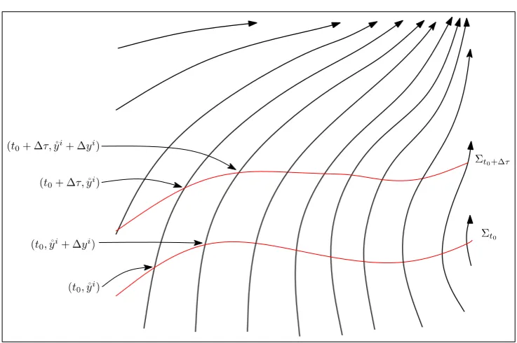
We will work in a comoving coordinate system yµ _{= (}_{t, y}i_{), one in which}

uµ _{= (1}_,₀_,₀_,_{0). Such a coordinate system can be constructed from a general}

coordinate system xµ_{in the following way (see Figure 3.1). Take a spacelike}

hypersurface Σt0 that crosses all the trajectories of fluid under consideration,

be it a small part of the manifold or the whole thing, and place coordinates

yi _{on the hypersurface. The fluid trajectories can then be given by} _xµ ₌

fµ₍_{τ, y}i_{), where} _yi _{is the coordinate on Σ}

(38)

Σt0

Σt0+∆τ

(t0+ ∆τ,˚yi)

(t0,˚yi)

(t0,˚yi+ ∆yi)

[image:38.595.134.503.120.365.2]

(t0+ ∆τ,˚yi+ ∆yi)

Figure 3.1: An illustration showing how one can construct a comoving coordinate system given the fluid trajectories parameterised by proper time,

τ, and then choosing an arbitrary initial foliation Σt0 with coordinates y i_.

proper time along the trajectory relative to the crossing of Σt0 at t = t0.

Therefore, we can recognise yi _{as Lagrangian coordinates. Provided there}

are no trajectory crossings, letting t = τ +t0, the inverse of fµ gives the comoving coordinates yµ _{in terms of the original coordinates} _xµ_.

Such a method gives constant time slices Σt that are dependent on the

choice of the initial constant time slice, Σt0. We can, however, in certain

situations define a unique constant time slicing as one will see in the next sections.

Given that gµνuµuν = −1, we have g00 = −1, so the metric takes the form

ds2 ₌₋_d_t2_{+ 2}_g

(39)

Orthogonal coordinates

When the flow is irrotational, we have the following three equivalent con-ditions [28]:

ωµν = 0, (3.32)

which is the definition of irrotational flow,

u[µ∇γuν]= 0, (3.33)

which is the condition that says uµ _{is hypersurface orthogonal, or}

equiva-lently

uµ=A ∂µB (3.34)

for some functions A and B of xµ. The level surfaces B =constant define the hypersurfaces orthogonal to uµ _and _A ₌ _±₍₋_gµν_∂

µB∂νB)−

1

2 _ensures

uµ_u

µ=−1, where the sign is chosen to make A ∂µB future pointed.

If we take B(yµ_{) =} _t_{, so that the hypersurfaces are those of constant}

time (but not necessarily proper time), then

uµ= (A,0,0,0), (3.35)

where A=−(−g00₎−1₂_{. Hence,}

uµ = (g00u0, g0iu0) (3.36)

= (₋1

A, C

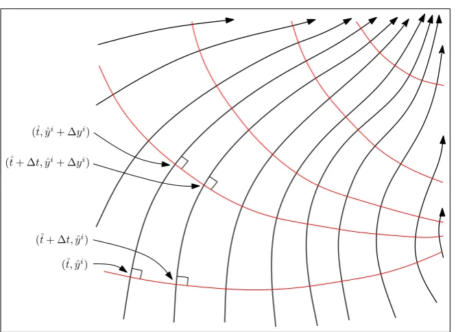
i₎_, _(3.37)

where Ci ₌ ₋_g0i₍₋_g00₎−1₂ _{are functions that will depend on how spatial} coordinates are placed on the hypersurfaces. Given that Ci ₌ dyi

dτ, where

τ is the fluid proper time, if we define the spatial coordinates such that the fluid stays at constant spatial coordinates, then Ci _{= 0. This is an}

orthogonal coordinate system (see Figure 3.2). We note yi _{need not be}

orthogonal to each other but just with the time coordinate, i.e., g0i _{= 0.}

In this coordinate system the metric is block diagonal, g0i ₌ _g

0i = 0,

g00_g

00 = 1, gijgik =δik and

ds2 ₌_g

(40)

(˚t,˚yi₎

(˚t+ ∆t,˚yi₎

(˚t,˚yi_{+ ∆}_yi₎

[image:40.595.154.487.122.364.2]

(˚t+ ∆t,˚yi_{+ ∆}_yi₎

Figure 3.2: An illustration showing how one can construct an orthogonal coordinate system given the fluid trajectories that are irrotational. We note that in 1+1 dimensions, as depicted, fluid flow is always irrotational.

Comoving orthogonal coordinates

When working with orthogonal coordinates, if dt

dτ =−

1

A = 1 then the time

coordinate t is equal to the fluid proper time and the coordinate system is also comoving. Such a choice is not possible in general, but can be made

when aµ _{= 0 in addition to} _ω

µν = 0, as we will now demonstrate. In an

orthogonal coordinate system,

aµ=uν∇νuµ =−A−1∇0uµ (3.39)

=−A−1∂0 −A−1

+ Γ0₀₀ −A−1,Γi₀₀ −A−1 . (3.40) One can show

Γ0₀₀= 1₂g00∂0g00 = ₂1(−A−2)∂0(−A2) = 1

A∂0A (3.41)

and

Γi

00=−12g

ij_∂

(41)

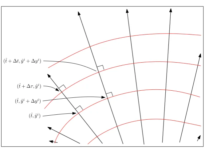
(˚t,˚yi₎

(˚t+ ∆τ,˚yi₎

(˚t,˚yi_{+ ∆}_yi₎

[image:41.595.109.443.118.358.2]

(˚t+ ∆t,˚yi_{+ ∆}_yi₎

Figure 3.3: An illustration showing how one can construct a comoving or-thogonal coordinate system given the fluid trajectories that are irrotational and geodesic. We note that in 1+1 dimensions, as depicted, fluid flow is always irrotational.

so that

aµ= (0, 1 Ag

ij_∂

jA). (3.43)

So, if aµ_{= 0, then}

∂iA= 0 (3.44)

which implies Ais constant with respect to the spatial coordinates, yi_{. We}

are free to define A(t) as we want as it is just a corresponds to a variable scaling of the time coordinate, t. Setting A =−1 we find that _dd_τt = 1 and

we have a comovingand orthogonal coordinate system, orGaussian normal

coordinates (see Figure 3.3). The metric takes the form

ds2 ₌₋_d_t2₊_g

(42)

3.3 Hypersurfaces

Consider an n-dimensional manifold, M, coordinates xµ_{, with metric} _g µν,

and a (n−1)-dimensional submanifold, a hypersurface N with coordinates

yα_{. The hypersurface can be given in}_M_{, either implicitly by the points at}

which a function, F(xµ_{), takes a constant value, or explicitly parametrized}

by the coordinates on N,xµ₌_ψµ₍_yα_{). The unit normal to the surface,} _η µ,

is then given by

ηµ=±

πµ

|gσρ_π σπρ|

1 2

, (3.46)

where

πµ=∂µF or πµ=µν1ν2···νn−1ψ ν1

,1ψν2,2· · ·ψ

νn−1

,n−1. (3.47)

One may then define the hypersurface projection tensor orfirst fundamental form,

Pµ_ν =δµ_ν₋σηµην, (3.48)

where σ =ηµ_η

µ denotes whether the normal is timelike or spacelike. It is

so called because its operation on tensors, denoted by a hat,

b

Aµν···ρσ··· =PµλPνκ· · ·PτσPυρ· · ·Aλκ···τ υ···· · · , (3.49)

can be shown to be orthogonal to the normal vector on every contraction,

b

Aµν···_ρσ_···ηµ=Abµν···ρσ···ην =Abµν···ρσ···ησ =Abµν···ρσ···ηρ =· · ·= 0. (3.50) It can be shown to act as the metric for vectors tangent to the hypersurface,

PµνVµWν =gµνVµWν (3.51)

where Vµ _and _Wν _{are tangent to the hypersurface. It also can be shown}

that it is idempotent,

Pµ_νPν_λ =Pµ_λ, (3.52)

(43)

3.4. The ADM gauge 31

If we have a family of hypersurfaces, as one would for the level sets of a function F(xµ_{), we have a vector field of hypersurface normals. We can}

then define the extrinsic curvature or second fundamental form, Kµν. It

describes how the projection tensor changes as we move along the integral curves of the normal vector field and is defined by

Kµν =−1₂LηPµν. (3.53)

One can then show this is equivalent to

Kµν =−PσµPρν∇(σηρ). (3.54)

Given coordinates on the hypersurface N, yα_{, such that} _xµ ₌ _ψµ₍_yα₎

defines the hypersurface, we can restrict or pullback any tensor in M to N

by

n−1_A

αβ··· =ψµ,αψν,β· · ·nAµν···, (3.55) where the n−1 _{pre-superscript denotes the pulled-back tensor in} _N _{of the} tensor in M denoted by the n _{pre-superscript.}

3.4 The ADM gauge

We will henceforth work in the ADM gauge for a Lorentzian manifold, M,

which is given in coordinates xµ_{= (}_{t, y}i_{). The hypersurfaces, Σ}

t, are those

of constant t, and the coordinates on the hypersurfaces are yi_{. The unit}

normal,mµ_{, which is timelike, is chosen to be future pointing. It is therefore}

given by

mµ = −

∂µt

(₋gσρ_∂ σt∂ρt)

1 2

= (−N,0,0,0), (3.56)

where N ≡ _√1

−g00 is known as the lapse function and

mµ=gµνmν =

1

N(1,−N

(44)

where Ni _≡ _g0i_N2 _{is the shift vector. One can then define the projection} tensor,

pµν =δµν +mµmν, (3.58)

=

"

0 0

Ni _δi j

#

, (3.59)

which projects tensors on to Σt and acts as the metric for tensors in the

hypersurface. One can show by raising an index on equation (3.58) and rearranging with the use of equation (3.57) that

gµν =

"

− 1

N2 N

j

N2 Ni

N2 pij− N

i_Nj

N2

#

. (3.60)

It is then possible, using the fact thatgµν_g

νλ =δµλ, to show that

gµν =

"

−N2₊_Nk_N k Nj

Ni pij

#

(3.61)

and

pijpjk =δik, (3.62)

whereNi =pijNj.

The pullback fromM to Σtis given in terms of∂x

µ

∂yi =δ

µ

i. Thus, equation

(3.55) gives

3_A

ij··· =4Aij···. (3.63)

We can use3_A

ij···and 4Aij···interchangeably but we cannot, however, inter-change tensors when some or all of the indices are raised, e.g.,

3_Ai

j···=3gik3Akj···6=4Aij···=giµAµj···, (3.64) in general. The equality only holds for tensors that are tangent to Σt, the

hypersurface projection tensor for example. When a tensor is only given with Latin indices without a pre-superscript we will henceforth assume that it is the component of the 3-tensor. We have the 3-metric on Σt,

3_g

(45)

Its inverse 3_gij _satisfies 3_gij3_g

jk = δik, so using equations (3.65) and (3.62)

we have

3_gij ₌4_pij ₌4_gij ₊ NiNj

N2 . (3.66)

We will therefore usepij andpij to denote the 3-metric on Σthenceforth. We

define the 3-covariant derivative,Di ≡3∇i, on Σtas the covariant derivative

given by the 3-Christoffel symbols, 3_Γi

jk, e.g., DiXj =∂iXj+3ΓkijXj etc.

The 3-Christoffel symbols are given in terms of the 3-metric, pij,

3_Γk

ij = 12p

kl₍_∂

ipjl+∂jpil−∂lpij). (3.67)

We also have the extrinsic curvature of Σt given by

Kµν =−pσµpρν∇(σmρ). (3.68)

One may show with the use of equations (3.56) and (3.59) that

Kµν =

"

−N Nk_Nl_Γ0

kl −N NkΓ0ik

−N Nk_Γ0

kj −NΓ0ij

#

(3.69)

Evaluating Γ0

ij, we can show

Kij =4Kij =

1

2N (DiNj +DjNi−∂tpij). (3.70)

Evaluating the rest of the Christoffel symbols we obtain all the independent ones,

4_Γ0

ij =−

1

NKij (3.71)

4_Γk

ij =3Γkij +

Nk

N Kij (3.72)

4_Γ0 00=

1

N ∂tN +N

i_D

iN −NiNjKij

(3.73)

4_Γk

00=pki∂tNi+N DkN −NiDkNi

− _N1 Nk∂tN +NkNiDiN

+N

i_Nj_Nk

N2 (2DiNj −N Kij) (3.74) 4_Γ0

i0 = 1

N DiN −N

j_K ij

(3.75)

4_Γk i0 =−

Nk

N DiN +DiN

k₊NkNj

N Kij −N K

k

(46)

We now also note the scalar Gauss equation [30],

4_R_{+ 2}4_R

µνmµmν =3R+K2−KijKij, (3.77)

where 4_R _and 3_R _{are the Ricci scalars of} _g

µν and pij respectively and K =

Ki i.

Comoving coordinates in the ADM gauge

Now if the coordinates are comoving with a fluid, we haveuµ _{= (1}_,₀_,₀_,₀₎

as the fluid 4-velocity andg00 =−N2+NkNk =−1. Using equation (3.61),

we then have

uµ=gµνuν = (−1, Ni), (3.78)

hµ_ν =δµ_ν +uµuν =

"

0 Nj

0 δi j

#

, (3.79)

Zµ_ν =_∇νuµ= Γµν0 (3.80)

and

aµ_≡uν_∇νuµ =Zµνuν = Γ µ

00. (3.81)

Also, one can show

Zij =4Zij =∇jui =DjNi−N Kij =D[jNi]+1₂∂tpij. (3.82)

So ifaµ _{= 0, as is the case for a geodesic dust fluid, then Γ}0

00 and Γk00 are zero. Also equation (3.3) gives

Z_µν⊥ =Zµν. (3.83)

and thus,

θij =4θij =D(jNi)−N Kij = 1₂∂tpij (3.84)

and

(47)

Comoving orthogonal coordinates in the ADM gauge

Now, if we have an irrotational geodesic fluid we can work in comoving orthogonal coordinates as is shown in §3.2. In this case the fluid 4-velocity is the hypersurface normal,

mµ=uµ= (1,0,0,0) andmµ=uµ= (−1,0,0,0). (3.86)

This implies N = 1, Ni _{= 0 and that the transverse projection tensor (3.1)}

and hypersurface projection tensor (3.58) coincide,

pµ_ν =hµ_ν =

"

0 0

0 δi j

#

. (3.87)

Equations (3.71) to (3.76) then give

Γ0_ij =₋Kij, 4Γkij =3Γkij, Γk0i =−Kki, Γ000= Γ0i0 = Γk00 = 0, (3.88) and equation (3.82) gives

Zij =−Kij = 1₂∂tpij. (3.89)

We can then show the rest of the components of Zµν are zero, as well as

θ_≡θµ_µ =θi_i = 1₂pij∂tpij (3.90)

and

σ2 ≡σµνσµν =σijσij = 1₄pijpkl∂tpik∂tpjl− ₁₂1 pij∂tpij

2

. (3.91)

Using (3.88) and (3.89), the covariant derivative along uµ _{can be shown to}

be

˙

Zij ≡uµ∇µZij =∂tZij −2ZikZkj. (3.92)

From equation (3.15) we see that

˙

Zij =−ZiρZρj−Riρjσuρuσ (3.93)

(48)

and, therefore,

∂tZij =ZikZkj−Ri0j0. (3.95)

Using the Ricci tensor for dust (3.21) we can show that the scalar Gauss

equation (3.77), in these coordinates, becomes the energy constraint for

dust,

16πGρ=3R+ 2 3θ

2

(49)

CHAPTER

4

Coarse-graining in general

relativity

4.1 Introduction to coarse-graining tensors

Thus far there exists no natural method for coarse-graining tensors (above rank zero) in a covariant manner. Efforts have been made by Zalaletdinov [31, 32] and others [33], but these generally require the addition of much mathematical structure over and above that provided by general relativ-ity. For a critical review of these approaches see, e.g., reviews of van den Hoogen [34], Ellis [35] and Wiltshire [12]. These methods also are not what we define as coarse-grainingper se; they are methods forsmoothing tensors. Smoothing defines a tensor field over the domain that is some continuous average of the original field, whereas coarse-graining defines a single aver-aged value of the original field. One could, however, choose the smoothed value at some single point as a coarse-grained value of the field.

4.2 Korzy´

nski’s method

Korzy´nski pushes the Newtonian cosmology analogy further by

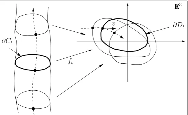
coarse-graining Zµν as was performed to va,b Chapter 2. Consider a finite fluid

(50)

38 Coarse-graining in general relativity

C

hZµνi

uα

∂Ct

Ct

∂C

[image:50.595.212.426.123.374.2]

t =const

Figure 4.1: A four-dimensional cylinder C, generated by the collective tra-jectories of a finite volume of fluid, and its boundary ∂Ct are foliated by

constant time slices. Image courtesy of Korzy´nski [13].

element travelling through spacetime (see Figure 4.1). The fluid element

defines a four-dimensional cylinder C in spacetime and its boundary ∂C

defines a three-dimensional tube. It can be foliated by suitably chosen constant time slices which will give three-dimensional spatial slices of the cylinderCtbounded by a two-dimensional spatial boundary ∂Ct. One may

then attempt to assign a coarse-grained value of Zµν for the domainCt. A

time evolution equation for the coarse-grained value of Zµν could then be

derived and it should have a similar form to (3.15) with additional terms derived from inhomogeneities in the metric and 4-velocity field. The addi-tional terms referred to as backreaction should reduce to zero for the FLRW solution as they did in the Newtonian case (2.73).

There are possibly unlimited ways in which one might assign a coarse-grained value toZµν on a domain, but some conditions should be placed to

(51)

4.2. Korzy´nski’s method 39

coarse-graining procedure should adhere to. The first condition states that if the volume of the fluid element is shrunk towards zero the coarse-grained velocity gradient should tend to the local one. The second condition states that such a procedure should be covariant in the sense that, apart from the choice of the fluid element itself and the 3+1 splitting of spacetime, the

result should not depend on any externally introduced structure, including

the coordinate system.

Korzy´nski does not explicitly state any further conditions. However, we will specify further natural conditions a coarse-graining procedure should

satisfy. When we coarse-grain a n-tensor we coarse grain over some n

-dimensional domain D on a n-dimensional (pseudo-)Riemannian manifold

M. When applied to cosmology, this manifold will usually be some spatial hypersurface as illustrated in Figure 4.1 with n = 3. The conditions are as follows:

1. When one wants to describe a coarse-grained tensor they must give the components of the tensor with respect to some basis or alternatively in some abstract tangent space. This also defines a metric that one can use to raise and lower indices, ¯g say. This basis or tangent space may or may not be related to some basis or tangent space on the manifold M.

If the coarse-grained tensor basis is not related to any basis on the manifold it should naturally have an orthogonal basis. This would mean hTiab···

cd··· should be unique up to orthogonal transformations,

hT_iab···_cd_··· = Λa_a0Λb_b0· · ·Λ−1c 0

cΛ−

1d0

d· · · hTi a0_b0

···

c0_d0_···, (4.1)

where

ηabΛaa0Λb_b0 =η_a0_b0. (4.2)

When averaging over a spatial constant time slice the canonical metric is ηab = diag(1,1,1) and Λaa0 ∈O(3).

(52)

40 Coarse-graining in general relativity

given that basis on the manifold. However one generally has the free-dom of choosing bases on a manifold so the coarse-grained tensor components generally will not be completely unique.

Either way, scalars which do not depend on a basis should be unique. Thus, scalars formed from grained tensors and the coarse-graining of scalars, e.g., _hT_iab···

ab···, hTiab···cd···hSicd···ab···,hUi, should be unique and not depend on the coarse-grained tensor basis.

The procedure should be covariant in the sense that the value of the coarse-grained tensor should not depend on coordinates placed on

M. The coordinates might give the basis and the components of the

coarse-grained tensor with respect to that basis. However, when one chooses different coordinates giving a different basis and components of the coarse-grained tensor, they should both be transformed the same way from the previous ones.

2. In the limit of the volume of the domain shrinking to zero around a point p the coarse-grained value should tend to the local value. In general, the coarse-grained tensor, _hT_iab···

cd···, and the local tensor,

Tαβ···_γδ_···, on the manifold will be given in different bases, so more formally there exists some matrixBa

α ∈GLn such that

hTiab···

cd···→BaαBbβ· · ·B−

1γ

cB−1δd· · ·T αβ···

γδ···|p (4.3)

as the coarse-graining volume is shrunk to zero around p. Moreover, ifTαβ···_γδ_···is given in an orthonormal basis atpandhTiab···

cd···is given in an orthonormal basis, Ba

α should be orthogonal i.e., satisfy (4.2).

(53)

4.2. Korzy´nski’s method 41

4. When coarse-graining a scalar the procedure should just be a plain volume-average over the domain. The 3-dimensional case being the Buchert average defined in _§5.2.

5. The procedure should be linear, that is,

haT +bSiab···

ab··· =ahTiab···ab···+bhSiab···ab··· (4.4) should be true for any tensors T and S and constant scalarsa and b.

The last three conditions we will not demand a coarse-graining procedure satisfy, but they are true in the flat case so one could demand them to possibly narrow down a number of coarse-graing methods that satisfy 1-4.

6. The coarse-grained metric, _hg_iab, should be the metric given by the

basis for the coarse-grained tensors, ¯gab.

7. The coarse-graining procedure should commute with contraction. That is, the following should hold,

hT_iab···_ad_···=_hTαβ···_αδ_···eˆβ· · ·ωˆδ· · ·ib···d···, (4.5)

where ˆeα and ˆωα are the basis vectors and dual vectors respectively

for T onM.

8. When coarse-graining over a domainD, composed of sub-domainsDi,

the coarse-grained tensor overDshould be some volume weighted sum of the coarse-grained tensor over the sub-domains Di. That is,

DhTi ab···

cd··· =

V1

V D1hTi ab···

cd··· ⊕

V2

V D2hTi ab···

cd··· ⊕ · · · , (4.6)

where V is the volume of D and Vi is the volume of Di such that

V = P_iVi. The summing operator ⊕ should reduce to the usual +

Average cosmic evolution in a lumpy universe

PHYS 690 MSc Thesis

The Degree of Master of Science in

Physics

Average cosmic evolution

in a lumpy universe

James A.G.

Duley

Supervisor:

Assoc. Prof. David L.

Wiltshire

Assistant Supervisor:

Dr Teppo

Mattsson

Contents

Acknowledgements

Conventions

CHAPTER

1

Introduction

1.1

Inhomogeneous cosmology

1.2

Thesis outline

CHAPTER

2

Newtonian cosmology

2.1

Introduction

2.2

Governing equations

Solving the system

The homogeneous case

2.3

Averaging of the Newtonian cosmology

CHAPTER

3

Congruences and the splitting

of spacetime

3.1

A kinematical description of spacetime

3.2

The 3+1 split of spacetime

Comoving coordinates

Orthogonal coordinates

Comoving orthogonal coordinates

3.3

Hypersurfaces

3.4

The ADM gauge

Comoving coordinates in the ADM gauge

CHAPTER

4

Coarse-graining in general

relativity

4.1

Introduction to coarse-graining tensors

4.2

Korzy´

nski’s method

_Duley

_Wiltshire