1
Technical Note: Defining prior probabilities for hydrologic
model structures in UK catchments
M. Clements1*, T. Wagener2, G. Coxon3, F. Pianosi2, J. Freer3 and M.J. Booij1
1Department of Civil Engineering, University of Twente, Horst, Enschede, The Netherlands 2Department of Civil Engineering, University of Bristol, Queen ‘s Building, Bristol, UK 3School of Geographical Sciences, University of Bristol, Bristol, UK
*Email for corresponding author: [email protected]
Abstract
Choosing a suitable model structure, i.e. a set of equations that represent the dominant hydrologic processes of interest, is the starting point for any modelling study. This model structure choice is often guided by experience with a particular model. More recently the focus has shifted to flexible modelling frameworks, which allow structures to be chosen based on the specific characteristics of the catchment under study. Little work has been done though on defining prior probabilities for different model structures based on physical catchment characteristics or climatic conditions. Here we combine two soil moisture accounting (SMA) modules used widely in the UK, PDM and Penman, in combination with three different routing modules, linear, parallel and leaky, and apply them to 89 UK catchments to define such prior probabilities. The 6 model structure combinations are applied in a Monte Carlo framework (10,000 parameter samples per structure) to each of the catchments and the fraction of parameter sets that are behavioural is estimated. Parameter sets are considered behavioural if they reach pre-‐defined thresholds regarding Nash-‐Sutcliffe Efficiency and Bias. We make the basic assumption that better model structures produce more behavioural parameter sets. We find that there is a clear distinction between model structures for different catchment types. A subsequent CART analysis quantifies how physical (baseflow index) and climatic (runoff coefficient) characteristics define which model structures are most likely.
We conclude that specific model structures work best for different catchments. We found that there is a certain classification of catchments possible per model structure combination. This classification can be determined by climate, topography, landuse and geology. Geology (BFI) in this case, determines which SMA module to use, while topography (DPSBAR), landuse and climate (Runoff Coefficient) determine which routing module to use.
Keywords: Model structure selection, prior probability
1. Introduction
2
Recent studies suggest that different systems might be best modelled using specific model structures (Clark et al., 2008; 2011). Examples of flexible model structures that have been proposed are the Rainfall-‐Runoff Modelling Toolbox (RRMT) developed by Wagener et al. (2001). This toolbox splits models into soil moisture accounting (SMA) and routing components and therefore makes the assumption that that the rainfall-‐ runoff process can be represented by these two components. Different model structures can then be selected for either of those components. The FUSE modelling framework (proposed by Clark et al., 2008) goes a step further by allowing even more flexibility than RRMT. The framework takes structural elements from several widely used hydrologic models (e.g. Topmodel) and allows the user to select any combination of these components. Different newer versions of this FUSE framework have been proposed such as the FLEX and the SUPERFLEX frameworks (Fenicia et al., 2007; Euser et al., 2013) The choice of the components are chosen by certain selection criteria. In this study we address the simple question: can we use a priori information to choose one or more model structures for a particular catchment?
Here we apply a combination of six different model structures made up of two different soil moisture accounting modules and three different routing modules. We assume that the chosen components are capable of representing the variability in physical characteristics that we expect to encounter within our dataset. We apply these models to 89 UK catchments to understand which model structure works better for different catchments.
In this paper, we first represent the variety in characteristics of the catchments to show that a wide range of catchments is used (chapter 2.1). We then show the different model structure combinations in detail (chapter 2.2). After that we introduce the methodology used for this research (chapter 3). The final results will be represented in figures and their physical interpretation will be discussed in detail (chapter 4). We finally conclude with some overall conclusions (chapter 5).
2. Data and Models
2.1 Catchment data
The used data from the catchments are respectively daily precipitation, potential evapotranspiration and discharge with a time series of 10 years. This data are from 89 catchments in Scotland, Wales and England with a surface area ranging from 0.9 km2 to
9895 km2 and with an average of 209 km2. The catchments have a wide range in
hydrologic characteristics. Some of these characteristics and the ranges of values found within the dataset are shown below:
• a base flow between 18% and 98%
• a runoff coefficient between 0.04 and 0.93
• a maximum elevation between 79 and 979 meters
3
suggesting significant differences in the response of the precipitation that becomes runoff.
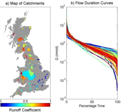
Figure 1; location of catchments used in this research and runoff coefficients(a) and their corresponding flow duration curves (b).
2.2 Hydrologic models structures
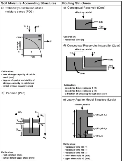
The models used consist of two separate modules: a Soil Moisture Accounting (SMA) module and a Routing module. They are implemented within RRMT discussed in the introduction section. All these modules are lumped, relatively simple (in terms of number of parameters), and of conceptual or hybrid metric-‐conceptual type (Wheater et al., 1993). The SMA module determines the actual moisture in the catchments. This results in an Effective Rainfall (ER). After the ER is calculated, the Routing module computes the amount of moisture that actual becomes runoff. In this study, two SMA modules and two routing modules are used. These will be described below, and an overview of these modules is shown in figure 2.
2.2.1 Soil Moisture Accounting model structures
Here we briefly explain the different model components used in this study. More details can be found in Wagener et al. (2001).
[image:3.595.73.484.109.489.2]
4
the stream. The Pareto Distribution will be used to take account for this response. The principle of this model is as follows: if rainfall is added to the component, the amount of moisture exceeding the critical capacity (cmax) will be the first contribution to the
effective rainfall, u1. This amount will be calculated by the following formula:
𝑢1! =max 𝑟!−(𝑐!"# −𝑐!!!) ,0)
Where:
rk = amount of rainfall
cmax = maximum capacity
ck-‐1 = capacity on time step k-‐1
k = time step
The remaining rainfall will than be added to the soil moisture store and redistributed between the stores based on a Pareto distribution (Wagener et al, 2001):
𝑠! = 𝑠!"# ∗(1− 1− min 𝑐!
𝑐!"# ,1.0
!!!
) Where:
sk= storage on time step k
smax = maximum storage
In this case, cmax, b and c(1) will be calibrated.
The stores that overflow produce the second part of the effective rainfall, u2. This part is computed by the following formula:
𝑢2! =max 𝑟!− 𝑠!−𝑠!!! ,0
5
[2] The ‘Pen model structure’, which is based on an empirical drying curve developed by Penman (1949). This structure is a two-‐store concept. The upper store (Smax) is equal to
the root constant and is calibrated. The other value that is calibrated is the initial deficit for the lower store. Beside these calibrated parameters, there are also parameters that
[image:5.595.72.494.72.626.2]6
are fixed. This is firstly the value of the lower store. This has been fixed to 1000 mm and is recommended by Moore (1992) and Jolley (1995). The reason for this is to make sure that the store doesn’t dry out.
The model structure also has a bypass mechanism. This accounts for the quick response of the catchment. This mechanism is fixed to 0.15 as recommended by Mander and Greenfield (1978, in Jolley 1995) and determines the precipitation that directly becomes runoff. There’s also a parameter that that defines the rate of the depletion after the upper store is emptied. This value is 0.08 (following Penman, 1949, in Jolley, 1995) i.e. the actual evapotranspiration reduces to 1/12 of the potential evapotranspiration. Before the store is emptied, this rate is 1:1.
Thus, this model structure has two calibrated parameters and three fixed parameters. The reason for the three parameters being fixed is that these have been found reasonable for catchments in the UK. A sketch of this structure is shown in figure 2(b).
2.2.2 Routing model structures The routing modules are as follows:
[1] The ‘Cres’ routing module is a single conceptual reservoir. A storage function is involved in the module, which describes the relationship between outflow of the reservoir and the amount of water stored,
𝑆 𝑡 =𝑎∗𝑄(𝑡)
where S(t) is the storage [L] at time t, a is a storage coefficient [L1-‐n * Tn], with n being the
coefficient of non-‐linearity. In this module, the reservoir will be assumed to be linear, so
n=1. Q(t) is the outflow [L/T]. The parameter that will be calibrated is the residence time [T]. This defines how long water is stored in the reservoir. The larger its value, the longer it takes for water to move through the reservoir and the more delay it produces. A sketch of this structure is shown in figure 2(c).
[2] The ‘2par’ routing module is a combination of two conceptual reservoirs as described above, in a parallel manner. The additional calibrating parameter is ‘alpha’ which is the fraction of ER that is going through one store. The remaining part will be the amount of moisture that flows through the other store, and reflects the groundwater of the specific catchment. A sketch of this structure is shown in figure 2(d).
[3] The ‘Leak’ module represents a leaky aquifer. This module is based on Moore (1999) who used a similar structure to model snow. The parameters that are calibrated are the residence times for each type of runoff and a lower threshold for the lower part q2 and
an upper threshold for the upper part q3 of the effective rainfall. The leakage from the
catchment is described by q1. In practice, this model represents catchments with a very
slow water flow component. A sketch of this structure is shown in figure 2(e).
3. Methodology
7
maximum values for each parameter and that the parameters follow a uniform distribution. We checked whether 10000 parameter samples is sufficient by repeating the sampling several. This made it visible whether the results were robust or not. The results were very similar, so an number of 10000 parameter samples is judged sufficiently reliable.
Furthermore, we selected some objective functions as basis for choosing acceptable models (chapter 3.1). With these objective functions we run the model structure combinations and consider the performance per catchment (chapter 3.2). In order to group different catchments we introduced some classifications (chapter 3.3). For a statistical reliable outcome we linked these groups of catchments a corresponding model structure combination with the use of Classification and Regression Tree analysis (chapter 3.4).
3.1 objective functions
We selected two objective functions as basis for choosing acceptable models. The first is the Nash Sutcliffe Efficiency. This metric has been introduced by Nash and Sutcliffe (1970) to allow the comparison of models applied to different catchments and to assess the value of additional or improved model components. Its range is from minus infinity to one, where one is its optimum. This function is defined as:
Where
o observed variable c calculated variable i time step
a) Routing structures
b) Soil Moisture Accounting structures
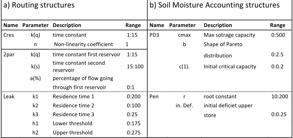
Name Parameter Description Range Name Parameter Description Range
Cres k(q) time constant 1:15 PD3 cmax Max sotrage capacity 0:500 n Non-‐linearity coefficient 1 b Shape of Pareto 2par k(q) time constant first reservoir 1:15
distribution 0:2.5 k(s) time constant second reservoir 15:100 c(1). Initial critical capacity 0:0.2
a(%) percentage of flow going
through first reservoir 0:1
Leak k1 Residence time 1 0:200 Pen r root constant 10:200 k2 Residence time 2 0:100 in. Def. initial deficiet upper k3 Residence time 3 0:25
store
0:0.25 h1 Lower threshold 0:175
h2 Upper threshold 0:275
RRMT User Manual
The following equation conventions are used in the OF equations: o observed variable
c calculated variable i time step
N total number of time steps available parameter set
3.5.1 Nash Sutcliffe Efficiency – OF_1_NSE
The Nash-Sutcliffe Efficiency (NSE) was introduced by Nash and Sutcliffe (1970, Garrick et al., 1978) to allow the comparison of models applied to dif-ferent catchments and to assess the value of additional or improved model components. It ranges from minus infinity to one, which is also the optimum value. A detailed analysis of the measure can be found in Legates and McCabe (1999). It is defined as
N i i N i i i o o c o . NSE 1 2 1 2 0 1
However, all objective functions in the RRMT have their optimum at a mini-mum value. The objective function calculated is therefore
NSE *
NSE 1
From the first equation it can easily be seen that an NSE value of zero indi-cates that the mean of the observed flow is an equally good predictor than the simulated flow sequence.
NSE puts higher emphasis on fitting the peaks of a hydrograph due to the use of squared residuals in its calculation.
3.5.2 Coefficient of Determination – OF_2_R2
The coefficient of determination R2 measures the proportion of the total vari-ance in the observations that can be explained by the model (Legates and McCabe, 1999). The measure has a range between zero and one, with one being the optimum value.
N i i N i i N i i i c c o o c c o o R 1 2 1 2 2 1 2
In order to minimize the value, the following adjustment to the measure is made,
2 1
2* R
R
See Legates and McCabe (1999) for more details on this measure.
3.5.3 Root Mean Squared Error – OF_3_RMSE The Root Mean Squared Error (RMSE) is defined as
45
[image:7.595.69.559.286.517.2]8 N total number of time steps
θ parameter set
In addition to the NSE metric, which is more focused on fitting the output variance, we add the absolute bias metric to account for the water balance fit. This value is at its optimum if it has the value 0. This metric is defined as follows:
We chose that parameter sets for a given model structure are considered acceptable (“behavioural”) if the associated NSE is higher or equal to 0.6, and ABIAS is lower or equal to 0.1. Any parameter set that falls outside these two thresholds is rejected.
3.2 Performance of structure combinations
During the calibration, all parameter sets that satisfied these thresholds are counted per model structure combination for each catchment. We made the basic assumption that per catchment, the structure combination with the largest number of behavioural parameter sets, is most likely to be a suitable representation of that catchment. With this data we achieve a list per catchment with the behavioural parameter sets per model structure combination. It is then easily visible which model structure will be best applicable to for a certain catchment.
3.3 Classification of catchments
In order to determine whether there is a correlation between certain characteristics of the catchments and the best working model structure combinations, certain characteristics of the catchments are chosen. These characteristics with its classes are shown below (Marsh and Hannaford, 2008):
Geology
For the representation of geology, the BFI per catchment is used. This is measuring of the amount of the runoff of the river that derives from stored sources (Gustard et al, 1992). Catchments with high base flow indices are likely to have a slow response, whereas catchments with low base flow indices are likely to have a fast response.
Landuse
The distribution of different use types of land per catchment, divided in: • Percentage of woodland
• Percentage of arable land • Percentage of grassland
Each type of land will have its own behaviour in terms of runoff. Catchments with a high amount of woodland or grassland areas will generally have a slower response of the discharge.
Climate
In order to represent the climate per catchment, firstly the Runoff Coefficient (Q/P) is used. This metric compares the amount of precipitation (P) to the amount of runoff (Q) over a certain period, in this case 10 years. In fact it is an average of how much of the
RRMT User Manual
N i i i c o N RMSE 1 2 1
It has the advantage that its values are in the same units as the data. Again, the use of squared values emphasises the fitting of high flows.
3.5.4 Absolute Bias - OF_4_ABIAS
Brazil (1988, p. 62) defines the absolute bias as follows
N i i N i i i o c o ABIAS 1 1
in this form it is also called volume error (Seibert, 1999, p19). The measure is implemented in OF_3_ABIAS.M in this form.
The measure can also be defined as mean error (Sorooshian et al., 1998) and is then written as
N i i i c o N BIAS 1 1
3.5.5 Heteroscedastic Maximum Likelihood Estimator – OF_5_HMLE
Sorooshian and Dracup (1981) introduced a Heteroscedastic Maximum Likeli-hood Estimator (HMLE) OF to account for the fact that the residuals usually increase with increasing flow values. This violates the assumption of a con-stant variance underlying for example the RMSE. They therefore define a weighted measure based on a Box-Cox transformation (Kottegoda and Rosso, 1997). The measure is calculated as follows
N / N i i N i i i i w c o w N HMLE 1 1 1 2 1
with the weights w being calculated as
1 2
i i f
w
where is the expected true flow value. Sorooshian and Gupta (1995, p.29) suggest to use the observed flow value as the expected true value. However, they warn that this will lead to a biased transformation parameter
i f
. has to be optimised in order to get a constant residual variance.
The following procedure (taken from Sorooshian and Gupta, 1995, p30) to es-timate is developed by Duan (1991):
9
precipitation becomes at the end runoff over the long term. Another way of representing the climate is by the Aridity Index (PE/P). This metric compares the potential evapotranspiration (PE) with the precipitation, and is therefore in fact an average of how much of the precipitation becomes potential evapotranspiration.
Topography
A descriptor of the topography is the mean Drainage Path Slope (DPSBAR). It provides an index of overall catchment steepness. This index is computed using the mean of all inter-‐nodal slopes for the catchment. It is expressed in metres per kilometre. Values of >300 m/km means that it is a mountainous terrain and values of <25 m/km are catchments with the flattest planes.
An overview of specific values per classification for each catchment is shown in appendix A and B.
In order to make sure that these characteristics aren’t strongly correlated, we plotted the values of the characteristics against each other. In these plots, there wasn’t a clear correlation visible between the chosen characteristics and therefore these characteristics are useful for the research. In addition to these plots, also the values of the aforementioned characteristics are plotted per model structure combination. It is than visible for which values per characteristic a certain model structure combination is best applicable. We then selected only the graphs that gave a clear preference for a certain structure combination. This is because the reason of the graphs is just to show that a correlation is visible rather then the physical reason for a specific correlation. In order to determine which graphs represent this distinction best, we plotted all values of all characteristics against each other. After that, we visually selected the graphs with the clearest distinction.
3.4 CART-‐analysis
3.4.1 tree building process
In order to make a more clear and statistical acceptable distinction between the different catchments and their best applicable model structures, we used Classification and Regression Tree (CART) analysis. This is a method that recursively splits the data until ending points, or terminal nodes. This is achieved with pre-‐set criteria. It analyses the explanatory variables and determines which division of the introduced variables best reduces deviance in the response variable (Lawrence and Wright, 2001). In this case it will be used for a classification of catchment characteristics into model structure combinations. For this analysis, firstly the ‘predictors’ or ‘independent outcomes’ are necessary. These are in this case the aforementioned catchments characteristics, such as BFI and Aridity Index. Secondly, the categorical outcomes, or ‘dependent’ variables are necessary. These are the best working model structure combinations. This outcome is associated with a certain weight. This is the third necessary variable and is the number of behavioural parameter sets per combination per catchment. (Lawrence, 2001). An overview of this number is shown in appendix C.
3.4.2 selection of a tree using Input Variable Selection
10
of independent variables (catchment characteristics). In that case, the chance that data points will be misclassified will decrease, at least on the dataset used for the CART calibration. However, the fewer variables are used, the more robust the CART is likely to be over different datasets, and also the clearer its interpretation will be. It is therefore necessary to find its optimal number of variables that should be used. The problem with finding its optimal number is that it is impossible to select this number a priori. For that reason, automatic procedures of Input Variable Selection (IVS) is used. IVS has been used in modelling water resources systems mainly to choose input of hydrological models and thus avoid unnecessary model complexity and enhances model accuracy (Galelli and Casteletti, 2013, Hejazi and Cai, 2009). This is the same principle necessary in our case; the only difference is that it is used for regression rather than classification. For this research, we already selected some characteristics a priori. These are listed on page 8 and 9. However, for the IVS analysis we introduced some more variables in addition to the ones already selected. The reason is that we wanted to be sure that there is a clear distinction between the variables that are superfluous and not. These added characteristics with a short description are listened below (Marsh and Hannaford, 2008).
• BFIHOST (transformation of BFI with soil type considered in percentage)
• Elevation (Height descriptor calculated by 10h percentile of elevation subtracted from 90th percentile of elevation in m)
• Area (the surface of the catchment in km2)
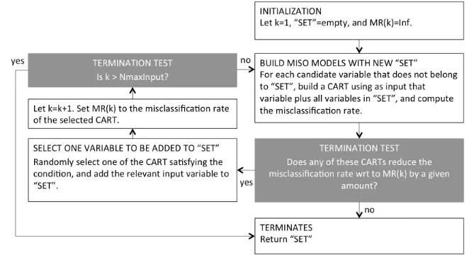
The IVS process works as follows. In the first stage, it builds a CART for each candidate variable. It then takes the variable with the smallest number of misclassified data points (variable 1). It then takes randomly the second variable (variable 2) and
analyses this
combination with CART. After this, it
compares the misclassified data points of this combination with the misclassified data points of variable 1. If the misclassified data points with this combination are decreased, it includes the regarding variable in its ‘best’ set of variables. If the misclassified data points with this combination are increased, it excludes the regarding variable and tries another variable. If there are no variables anymore that give a better performance, the process will be terminated. An overview of this principle is given in figure 5.
3.4.2 the final tree
When the selected variables are implemented, CART software finds the best way of splitting the variables by checking all possibilities. After that, it creates a tree with one of the variables on each node. The branches represent certain criteria for each variable. By
[image:10.595.194.525.371.551.2]11
comparing these criteria to the values of a certain catchment, a certain ‘route’ on the tree can be followed. At the end of this ‘route’ the optimal model structure combination will appear.
3.4.2 advantages and disadvantages of CART
The advantage of CART is that it is inherently non-‐parametric in the first place. It is therefore applicable to a wide variety of analyses. Also, it can be used with many possible predictors. CART has a sophisticated system to deal with enormous numbers of different variables and is therefore also useful for this classification problem. Furthermore, it has clever methods for dealing with missing variables and a relatively little input is required from the analyst. Finally, the trees are relatively simple to interpret. A disadvantage is that it is an automated strategy, which depends on the choices made. However, for this research it has been very helpful and it also compares the classified with the misclassified data points, which makes it therefore a robust approach.
4. Results and Discussion
4.1 Results
In this section, we discuss the main results supported by the figures presented here. Some further details are shown in the appendix and are referred to as appropriate in the text.
4.1.1 Performance of structure combinations
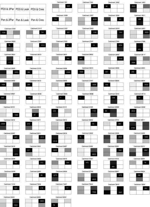
The result of the performance of the structure combinations per catchments is plotted in six squares, each representing a certain model structure combination (figure 6). The darkness of each square represents the number of behavioural parameter sets relatively to the maximum number per catchment (darker colour means larger number). This maximum number is shown in the square of the regarding model structure combination. The station number of each catchment is represented on top of each square plot. This number and its corresponding catchment name are shown in appendix A and B.
In the figure we find that the model structure with the highest number of acceptable parameter sets varies across the catchments, therefore suggesting that model structure selection is important. The lowest number of acceptable parameter sets that defines the chosen model structure is 1, while the highest number is 9321. Furthermore, the structure combination most often chosen is PD3 & Cres, while the least often chosen structure combination is Pen & 2par. Also it is visible that, for the Soil Moisture Accounting structure, the Probability Distribution (PD3) structure is more often selected than the Penman model structure. From the routing model structure, the Leak structure is chosen least and the Cres structure is chosen most often. It is therefore clearly visible that there is a certain difference across the best working model structures.
4.1.2 Classification of catchments
In order to know whether there’s a correlation between certain specific catchments and their best applicable model structure combination, some of the values of the characteristics are plot against each other. This is shown in figure 7.
12
Figure 6; Performance for every model structure combination per catchment. Every square represents such a combination, with its location shown in the square plot on the far top left. The black square represents the best working model structure combination, and the number in it is the number of behavioural parameter sets (out of 10000). The grey colour in the other squares give an indication of the number of behavioural parameter sets of that specific structure combination, relative to the best model structure.
[image:12.595.57.557.50.738.2]13
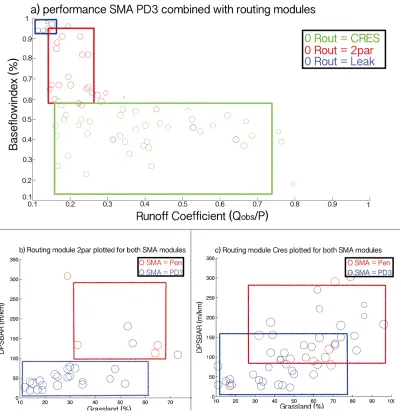
In the figure, every data point in the graph represents a catchment. The colour is determined by the best performing routing or SMA model structure. The size of the data point is proportional to the number of behavioural parameter sets. Fig. 7(a) shows the cases where PD3 is the chosen soil moisture accounting structure.
We find that the Leak routing structure is needed for catchments with a high baseflow index and a low runoff ratio, RR. Reducing the BFI (down to about 0.55) and increasing the RR up to about 1 leads to a patch in which the parallel routing structure is preferred (2par). Reducing the BFI value further leads to Cres being the preferred routing structure. Fig 7(b) shows the case where 2par is the chosen routing module and Pen and PD3 the soil moisture accounting modules. Fig. 7(c) shows the same combination, but
[image:13.595.76.477.171.588.2]14
Cres as the chosen routing module rather then 2par. In both cases we find that the SMA structure PD3 is needed for low values of DPSBAR and percentages of grassland area, while for higher values of these descriptors Pen is the preferred SMA structure.
4.1.3 selection of a tree using Input Variable Selection Table 2 shows the result of the IVS analysis.
For each attempt, the combination of characteristics that gave the best performance are coloured with grey squares. Also, the number of misclassified data points is shown for each attempt.
The variables that led to the least misclassified data points in the tree were attempt 4 and 14. The corresponding combination consists of the following characteristics: the baseflowindex, area of grassland, DPSBAR, area of woodland and the runoff coefficient. This means that to achieve the best balance between the complexity and robustness of the tree, the selection made before the use of CART was a good selection. The only difference is that the aridity index and the surface of arable land were not necessary.
4.1.4 the final tree
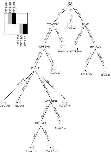
Figure 8 shows the final decision tree that is created with CART analysis. In this tree it is visible that geology, land-‐use, climate and topography are represented.
In the tree, there is also the percentage of classified and misclassified data points is presented. This is done by a bar plot. In this plot the tallest bar is the model structure combination that is chosen by CART. In some cases, some lower bars are plotted in the same graph. These smaller bars represent the number of misclassified data
points relatively to the chosen structure combination. It is now visible how robust the choice for a certain structure combination is.
The baseflow index in this case is mainly responsible for the choice of the type of routing module. In the first stage, BFI splits into three parts with each part leading to a different type of routing module. It is also visible that catchments with a high baseflow index but a low runoff coefficient will best perform if a Leak structure will be used. If there is a higher baseflow index and a high runoff coefficient, routing module 2par will be best applicable. Furthermore, catchments with a lower baseflow index will be best represented with the routing module Cres. This was already visible in figure 7(a), where the baseflow index was plotted against the runoff coefficient.
#"Misclassified Datapoints 1 12 2 9 3 10 4 7 5 12 6 13 7 13 8 13 9 13 10 14 11 9 12 10 13 10 14 7 15 8 16 10 17 10 18 10 19 11 20 13 Ar ab le
Area Arid
ity BF I BF IHO ST DP SBA R El ev ati on G ras sl an d Ru n. "C oe ff . W oo dl an d Atte m pt Results"IVS"analysis"
[image:14.595.308.535.318.582.2]15
Figure 8; The decision tree that is created with the CART analysis. With this tree a decision can be made about the best model structure combination that could be used, depending of the characteristics of a specific catchment. This can be done by following a route by selecting the applicable values of the characteristics of a certain catchment. Also, in the bar plots the reliability of the choice for a certain model structure combination is shown.
Hence it is visible that topography will determine which soil moisture accounting module should be used. In general, catchments with high values of DPSBAR will be best represented with the Penman model structure, while catchments with low values of DPSBAR will work with the Probability function. This was already visible in the 7ures 7(b) and 7(c).
[image:15.595.76.451.66.579.2]16
woodland. Also when the catchment is mainly covered with grassland, the Penman structure will work best.
4.2 Discussion
In this section we discuss why the different modules can be used best. We determined this by the use of the tree in figure 8 and figure 7. However, in this section we only discuss the results of the tree as this is a more extended and robust presentation of figure 8 and it shows in principle the same.
In the first place, it is clearly visible that the baseflow index in combination with the runoff coefficient makes the distinction between which routing module to use.
The reason that the routing module Cres works best for catchments with a low baseflow index is that the response of the precipitation is very much related to the discharge. In order to describe this behaviour, just a conceptual reservoir is necessary as it just computes the residence time that defines how long the water is stored in the reservoir. However, if this response is not that quick, an extra conceptual reservoir component is necessary. This computes two different residence times for each reservoir, where one reservoir is for quick responses whereas the other is for less quick responses. This principle is necessary for catchments with moderate baseflow indices. If there are catchments with a very slow response, even a third component with a third residence time is necessary. In that case, the Leak component will work best. This is the case for catchments with very high baseflow indices, or very low runoff coefficients. In these catchments there is always a discharge in the river, even in the driest periods. In that situation, the water comes from deep flows. The Leak structure also allows for losses, i.e. it allows for some of the precipitation leaving the catchment through subsurface pathways, rather than through the river and the catchment outlet.
In the second place, it is also clearly visible which SMA modules to use. This is mainly determined by the DPSBAR and the different types of landuse.
The Penmen structure allows for different types of vegetation cover (reflected in the size of the upper store) to be represented and to have an impact on the amount of actual evapotranspiration that occurs. It therefore reflects relatively homogeneous areas very well. This is also visible in the tree as Penman is the chosen model structure for high catchments with high values of altitudes (DPSBAR) and high values of different types of landuse. It also has a bypass component that allows for quick contributions to runoff. The PD3 model allows for spatial variability in response within a catchment due to its probability distribution of soil moisture depths. Hence it reflects more heterogeneous catchments better, which is visible in the tree by low values of altitudes and different types of landuse. This is likely more often the case than a homogeneous land use as the PD3 structure is chosen more often.
5 Conclusions
17
However, there are a few subjects that can be considered in further research. Firstly, we only used a selection of structures that are applicable to the UK. In further research, this subject can be extended by the use of more structure combinations. Secondly, the Penmen model structure provided good results less often than expected. Further research could get into more detail why a distribution function works better than a function that basically is adapted to the physical characteristics of catchments. Also, in this research the RRMT user manual is used which allows the choice of different model structure combination. However, in further research this can be extended by the use of the FUSE (with its extensions FLEX and SUPERFLEX) that allows even more flexibility.
Acknowledgements
We thank the Environment Agency of the UK for providing the data used in this study.
18
References
Clark, M., Slater, A., Rupp, D., Woods, R., Vrugt, J., Gupta, H., Wagener, T. and Hay, 2008. Framework for understanding structural errors (FUSE): A modular framework to diagnose differences between hydro-‐ logical models, Water Resources Research, 44, W00B02, doi: 10.1029/ 2007WR006735.
Clark, M., Kavetski, D. and Fenicia, F. 2011a. Pursuing the method of multiple working hypotheses for hydrological modeling, Water Resources Research, 47, W09301, doi:10.1029/2010WR009827.
Euser, T., Winsemius, H. C., Hrachowitz, M., Fenicia, F., Uhlenbrook, S. and Savenije, H. H. G., 2013, A framework to assess the realism of model structures using hydrological signatures, Hydrology Earth System Sciences, 17, 1893-‐1912, doi:10.5194/hess-17-1893-2013
Fenicia, F., Savenije, H. H. G., Matgen, P., and Pfister, L.: A comparison of alternative multiobjective calibration strategies for hydrological modelling, Water Resources Research, 43, W03434, doi:10.1029/2006WR005098, 2007.
Galelli, S. and Catellitti, A.,2013. Tree-‐based iterative input variable selection for hydrological modeling. Water Resources Research, doi: 10.1002/wrcr.20339 Gustard, A., Bullock., A. and Dixon, J.M., 1992. Low flow estimation in the United
Kingdom. Institute of Hydrology, Report No. 108, 20.
Hejazi, M., I. and Cai, X., 2009. Input variable selection for water resources systems using a modified minimum redundancy maximum relevance (mMRMR) alogarithm. Elsevier, 32 (4), 582-‐593.
Jolley, T.J. 1995. Large-‐scale hydrological moddeling -‐ The development and validation of improved land-‐surface parameterisations for meteorological input. Ph.D.
Dissertation, Imperial College of Science, Technology and Medicine. London, U.K., Unpublished.
Lawrence, R. L., Wright, A., 2001. Rule-‐Based Classification Systems Using Classification and Regression Tree (CART) Analysis. Photogrammetric Engineering & Remote Sensing, 67(10), 1137-‐1142
Mander and Greenfield (1978) – see Jolley (1995)
Marsh, T. J. and Hannaford, J. (Eds). 2008. UK Hydrometric Register. Hydrological data UK series. Centre for Ecology & Hydrology. 210 pp.
Mroczkowski, M., Raper, P. and Kuczera, G.,1997. The quest for more powerful validation of conceptual catchment models, Water Resources Research, 33(10), 2325–2335
Moore, R.J. 1992. Hydrological models -‐Nonlinear storage models. International Course for Hydrologists, International institute for Hydraulic and Environmental Engineering, Intstitute of Hydrology, Wallingford, U.K.
Moore, R.J., 1999. Real-‐time flood forecasting systems: Perspectives and prospects. In Casale R. and Margottini C. (eds.). Floods and Landslides: Integrated risk assessment.
Springer-‐Verlag, Berlin, 147-‐189.
Nash, J.E., and Sutcliffe, J.V., 1970. River flow forecasting through conceptual models I. A discussion of principles. J. Hydrol., 10, 282-‐292.
Penman, H.L. 1949. The dependence of transpiration of weather and soil conditions. Soil Science, 1, 74-‐89.
Uhlenbrook, S., Seibert, J., Leibundgut, C. and Rodhe A., 1999. Prediction uncertainty of conceptual rainfall-‐runoff models caused by problems in identifying model parameters and structure, Hydrologic Science Journal, 44(5), 779– 797.
19
Sivakumar, B., 2008. Dominant processes concept, model simplification and
classification framework in catchment hydrology, Stochastic Environmental Research Risk Assess, 22(6), 737–748.
Wagener, T., Lees M. J., Wheater, H. S., 2001. A framework for development and application of hydrological models. Hydrology & Earth System Sciences, 5(1), 13-‐26. Wagener, T., McIntyre, N., Lees, M., Wheater, H. and Gupta, H, 2003. Towards reduced
uncertainty in conceptual rainfall-‐runoff modeling: Dynamic identifiability analysis,
Hydrologic Process, 17(2), 455–476.
Wheater, H.S., Bishop, K.H. and Beck, M.B., 1986. Progress and directions in rainfall-‐ runoff modelling, In: Modeling change in environmental systems (EDS. A.J. Jakeman, M.B. Beck and M.J. McAleer). 101-‐132. Wiley, Chichester, U.K.
20
Appendix A; Physical characteristics of used catchments i.e. river name, station name, area and DPSBAR.
Station number River name Station name Catchment Area (km2) DPSBAR (m/km)
1001 Wick Tarroul 161,9 30 7005 Divie Dunphail 165 77 10002 Ugie Inverugie 325 42 14001 Eden Kemback 307,4 73 15008 Dean Water Cookston 177,1 59 15027 Garry Burn Loakmill 20 111 16004 Earn Forteviot Bridge 782,2 156 18011 Forth Craigforth 1036 (-‐) 21003 Tweed Peebles 694 181 21013 Gala Water Galashiels 207 149 21027 Blackadder Water Mouth Bridge 159 57 23003 North Tyne Reaverhill 1007,5 92 23018 Ouse Burn Woolsington 9 30 25001 Tees Broken Scar 818,4 82 26005 Gypsey Race Boynton 240 51 27007 Ure Westwick Lock 914,6 99 27023 Dearne Barnsley Weir 118,9 74 27047 Snaizeholme Beck Low Houses 10,2 204 27059 Laver Ripon 87,5 65 27088 Calder Mytholmroyd 171,7 144 28001 Derwent Yorkshire Bridge 126 191 28019 Trent Drakelow Park 3072 34 28031 Manifold Ilam 148,5 117 28050 Torne Auckley 135,5 21 28082 Soar Littlethorpe 183,9 26 28117 Derwent Whatstandwell 755 133 30003 Bain Fulsby Lock 197,1 39 31016 North Brook Empingham 36,5 32 32008 Nene/Kislingbury Dodford 107 42 33013 Sapiston Rectory Bridge 205,9 19 33033 Hiz Arlesey 108 36 33051 Cam Chesterford 141 41 34002 Tas Shotesham 146,5 20 34012 Burn Burnham Overy 80 27 36005 Brett Hadleigh 156 30 37007 Wid Writtle 136,3 27 38003 Mimram Panshanger Park 133,9 44
38020 Cobbins Brook Sewardstone Road 38,4 44
21
Station number River name Station name Catchment Area (km2) DPSBAR (m/km)
39007 Blackwater Swallowfield 354,8 32 39030 Gade Croxley Green 184 54 39065 Ewelme Brook Ewelme 13,4 78 39086 Gatwick Stream Gatwick Link 33,6 48 39101 Aldbourne Ramsbury 53,1 89 39114 Pang Frilsham 89,8 56
39131 Brent Costons Lane Greenford 146,2 34 40012 Darent Hawley 191,4 71 41011 Rother Iping Mill 154 75 41025 Loxwood Stream Drungewick 91,6 56 42008 Cheriton Stream Sewards Bridge 75,1 54 43006 Nadder Wilton 220,6 79 43018 Allen Walford Mill 176,5 52 44011 Asker East Bridge Bridport 48,5 138 45012 Creedy Cowley 261,6 111 46005 East Dart Bellever 21,5 95 47013 Withey Brook Bastreet 16,2 81 48011 Fowey Restormel 169,1 113 50007 Taw Taw Bridge 71,4 95 50011 Okement Jacobstowe 82,1 130 52016 Currypool Stream Currypool Farm 15,7 134 53002 Semington Brook Semington 157,7 48 53008 Avon Great Somerford 303 29 54002 Avon Evesham 2210 38 54018 Rea Brook Hookagate 178 90 54041 Tern Eaton On Tern 192 36 54057 Severn Haw Bridge 9895 73 54090 Tanllwyth Tanllwyth Flume 0,9 155 55002 Wye Belmont 1895,9 134 55013 Arrow Titley Mill 126,4 130 55026 Wye Ddol Farm 174 180 55034 Cyff Cyff flume 3,1 183 56019 Ebbw Brynithel 71,7 188 57007 Taff Fiddlers Elbow 194,5 153 57015 Taff Merthyr Tydfil 104,1 157 58005 Ogmore Brynmenyn 74,3 222 60006 Gwili Glangwili 129,5 150 64001 Dyfi Dyfi Bridge 471,3 270