JEEECCS, Volume 6, Issue 22, pages 1-8, 2020
A Decoupled Digital Feedback Control
Architecture for Input-Delay Robotic
Servomechanisms:
Design and Simulation
Loga Nga Fouda Jeanne
Research Laboratory of Computer ScienceEngineering and Automation ENSET, University of Douala
Douala, Cameroon [email protected]
Mbihi Jean
Research Laboratory of Computer Science Engineering and Automation ENSET, University of Douala
Douala, Cameroon [email protected]
Kom Charles Hubert
Research Laboratory of Computer Science Engineering and Automation ENSET, University of Douala
Douala, Cameroon [email protected]
Abstract – This paper presents a decoupled feedback
control architecture, for input-delay robotic
servomechanisms. As a decoupling principle, any servomechanism is modeled by a local input-delay dynamic model. However, the coupling effect from the motion of other servomechanisms, locally acts as an unknown and bounded disturbance to be rejected by a robust digital PIDF (proportional derivative, integral with filer) controller. As a beneficial implication, the proposed digital feedback control architecture, is designed and simulated according to methodologies and tools available in the literature for siso (single-input
single-output) input-delay control servo-systems.
Simulation results obtained from prototyping
servomechanisms are presented and discussed. These results show the high precision and robustness, of the
proposed decoupling digital feedback control
architecture. In future research works, the software code of digital PIDF controllers, will be implemented and uploaded into a DSP (digital signal processing) target, e.g., FPGA chip, for digital control of real input-delay robotic servomechanisms.
Keywords-servomechanisms; decoupled feedback control; bounded disturbance; digital PIDF controller; precision and robustness.
I. INTRODUCTION
The servomechanisms are encountered in a wide variety of application areas, including vehicles, machine tools, motorized conveyors, automated manufacturing, motorized water pumps, maritime and space navigation engines, both agriculture and home automation, and specially fixed and mobile robotics.
In the case of robotic servomechanisms, their increasing popularity is mainly due to low cost, ease of maintenance, interfacing flexibility with DC energy sources (e.g., battery, photovoltaic panel or both), fidelity, better production efficiency, while simultaneously maintain high precision, and a great operational robustness.
In addition, compared to human operators, the robotic servomechanisms can rapidly perform tedious tasks, involving artificial intelligence capabilities. However, they are intrinsically nonlinear, and structurally multivariable dynamic systems. As an implication, the complex nature of robotic systems has been and remains a mayor difficulty for the development of both low cost and reliable feedback control policies.
motion of other servomechanisms. As an implication, independently of the modeling tools (e.g. Euler-equations and Lagrange laws), a rigorous dynamic model of a robot, consists of a set of coupled kinematic and dynamic nonlinear equations [3-5]. Therefore, the design of feedback control schemes from such complex and intricate dynamic models, has been and remains an active research area for both fixed and mobile robotics [6-10].
The main feedback control schemes encountered frequently in robotic control systems, can be classified into three relevant categories as follows:
a) Multivariable nonlinear control scheme: It is based on exact linearizing and decoupling feedback, of the coupled dynamic state model. The related motion equations built in the state space, are linearized and decoupled by appropriate nonlinear feedback. This architectural approach leads to a precise open loop model. However, it involves complex equations, requiring enormous computing power. Therefore, are difficult to materialize in most practical contexts. It also requires powerful digital computing resources for the implementation of the resulting controllers [11-12].
b) Multivariable input-output nonlinear control scheme: It is based on exact transform of the coupled nonlinear dynamic model, into m
equivalent decoupled siso canonical models (one for each degree of freedom). This requires enormous computing resources due to Lie Brackets calculus [13].
c) Decoupling linear control scheme: based on an approximate decomposition into decoupled dynamic servo-systems. In which case the coupling effect due to the motion of other servomechanisms, is treated as disturbance. This is easy to design, however, might become utopic and unrealistic if servo-actuators involve some intrinsic and intricate behaviors, e.g., dead zone, input delay, etc. This approach leads to simplified models, therefore, practical for the implementation of the feedback controller. Here, one no longer needs to apply the complex nonlinear control scheme. Then, the intricate computation of the robot's reverse dynamics is avoided. Although advantageous by its simplified nature, it might create a significant behavior gap, compared to the physical reality of a whole robotic servomechanism. In which case, a simple feedback with low cost implementation, is unable to stabilize, neither a local servo-system nor a whole robotic servomechanism.
Following the previous literature review, the aim of this paper is to design and simulate a decoupled and piecewise linear digital feedback control scheme, for input-delay robotic servomechanisms. In each decoupled input-delay servomechanism, the coupling
effect from the motion of other, is treated as an
unknown disturbance with bounded magnitude. Moreover, a simple digital PIDF controller per each locally decoupled servomechanism, is synthetized and used in order to meet our twin objectives, of tracking any reference output and rejecting any unknown disturbance with bounded magnitude. The advantages of the new control architecture are as follows:
a) The feedback control problem can be systematically solved, according to design methods and tools of robust controllers, for siso (single input and single output) input-delay servo-systems [14-15].
b) The robotic servomechanism is decomposed into M decoupled siso dynamic servo systems, in which M servo actuators now have intrinsic realistic behaviors, such as dead zone and input delay. To this, is added the coupling effect of the motion of other servo systems. This keeps the whole robotic servomechanism model, fairly closed to that of the physical reality.
c) The PIDF controller to be used for each decoupled servo-system, is structurally simple, and can be easily embedded on DSP chips. d) Compared to a standard PID controller, the
proposed PIDF feedback control policy, is highly robust for both disturbances tracking and uncertainties rejection.
The next sections of this paper are organized as follows: In section II, are presented the methodology and tools used to design and simulate the proposed PIDF-based feedback control architecture, for input-delay robotic servomechanisms. In Section III, the simulation results obtained from prototyping servo-systems are presented and discussed. Finally, the conclusion of the paper is provided in section IV.
II. METHODOLOGY AND TOOLS
A. Decoupled Dynamic Model of Input-Delay Robotic Servomechanisms
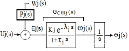
The decoupled dynamic model of input-delay robotic servomechanisms, is presented in Figure 1. The subscript j = {1, 2,…, M} is an index variable of an any servomechanism.
Figure 2. Decoupled model of the feedback control scheme of input-delay servomechanism
The symbols used in figures 1 and 2, are: ▪ λj: time delay;
▪ Kj: static gain; ▪ Τj: time constant;
▪ Uj, Yj: control input and output respectively;
▪ ωj : speed variable ▪ ϴj : position variable
▪ Wj : coupling disturbance(torque or force) ▪ Ej = Uj
+
PjWj : tracking error▪ Pj: transfer function on the disturbance ▪ Gcj(s): Open loop transfer function of the
decoupled dynamic model
A complete list of symbols is provided in the nomenclature, before reference section of this paper. Given these parameters, the open loop transfer function of the decoupled dynamic model presented in figure 1, is given by:
s) s ( )
(1 s
j j j
e Gc s Kj
−
=
+ (1)
The unknown parameters in equation (1), can be experimentally determined, using Strejc identification technique [16], for an input-delay servomechanism, under step response with speed as output.
B. Decoupled Analog Feedback Control Scheme of Input-Delay Robotic Servomechanisms
The decoupled analog feedback control scheme, of the robot with M input-delay servomechanisms, is shown in figure 2, where the transfer function of the PIDF controller is given by (2).
The transfer function of the PIDF controller observed in figure 2, is given by:
E (s) s 1+T s
( ) s
( )
s 1
1+T s
1
j dj
j pj
j fj
K
U s ij K Dc s K
Tdj K pj T s
ij fj = = + = + +
+
(2) where,T , T
K
K pj dj
ij K dj K
ij pj
= = (3)
and Kpj, Tij and Tdj being, of course, being proportional gain, integral time constant, and derivative time constant respectively.
Figure 3. Equivalent digital feedback control scheme
Figure 3 is, of course, an equivalent discrete representation of the same feedback control scheme. According to the control engineering practice, if Gjc(s) and Djc(s) are known, then the analog feedback control system shown in figure 2, could be preliminary designed, and simulated in the analog domain, in order to appreciate the predicted qualities of the closed loop servo-systems. Assuming that, these predicted qualities obtained in the analog domain are satisfactory, then, the next step is to compute the discrete transfer functions Gj(z) and Dj(z) from Gcj(s) in equation (1) and Dcj(s) in equation (2), respectively.
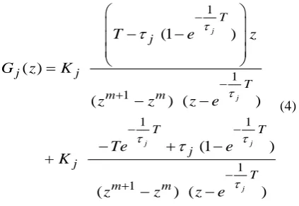
C. Synthesis of Decoupled Discrete Feedback Control Scheme
The transfer discrete function, Gj(z)observed in figure 3,is usually computed from Gjc(s) using the
modified m-order z-transform technique. Therefore,
Gj(z) is given by [14-15]:
1 1 1 1 1 1 1 (1 ) ( ) ( ) ( ) (1 ) + ( ) ( ) j j j j j T j j j T m m T T j j T m m
T e z
G z K
z z z e
Te e
K
z z z e
− − + − − − + − − = − − − + − − −(4) [5.28]
On the other hand, Dj(z), computed from Dcj(s) using
Tustin discretization method, is also given by [19]:
2
0 1 2
2
1 2
( )
( ) pj j j j
j j
b z b z b D z K
z a z a
+ +
=
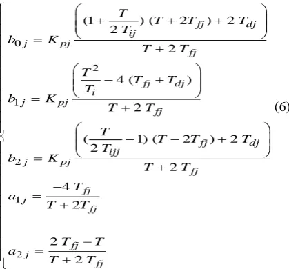
The resulting discrete transfer function of the
PIDF controller, is calculated under a sampling period T with parameters b0j, b1j, b2j, a1j and a2j, given by equation (6).
0 2 1 2 1 2
(1 ) ( 2 ) 2
2
2
4 ( )
2
( 1) ( 2 ) 2
2 2 4 2 2 2 fj dj ij j pj fj fj dj i j pj fj fj dj ijj j pj fj fj j fj fj j fj T
T T T
T b K T T T T T T b K T T T
T T T
T b K T T T a T T T T a T T + + + = + − + = + − − + = + − = + − = + (6)
In equations (4) and (5), however, the sampling Frequency T used for the discretization, should be chosen according to Nyquist sampling theorem [17].
D. Dynamic modelling and simulation tool
The simulation of the analog feedback control scheme given (1) and (2-3), and its equivalent discrete version given in (4) and (5-6), requires an advanced software tool, for the experimental modeling of open loop transfer function for input-delay dynamic models, and for conducting reliable simulations of siso input-delay control system.
In this paper, we resort to our proprietary virtual instrumentation and automation software, “GuiMexServoSys” developed in previous works
conducted in our research laboratory, and published with more deep details, in many references [18-19].It is a high level visual 32/64 Windows application, built form a mix of Matlab/GUI and Matalb/MEX-C++ technologies. Moreover, it is equipped with ready-to-use resources for rapid simulation and monitoring of analog and digital input-delay systems, from transfer functions or state space dynamic models, as it will be seen in the next section.
III. RESULTS AND DISCUSSIONS
A. Parameters of Prototyping Servomechanisms
For prototyping systems, it is assumed, without loss of generality, that the servomechanisms have the same following parameters:
▪ λ = λ1 = λ2 = . . ., λj, …, λn: time delay; ▪ K = K1 = K2 = . . ., Kj, …, Kn: static gain; ▪ τ = τ1 = τ2, . . ., τj, …, τn : time constant; ▪ P = P1, p2, …, Pj, …, Pn: for disturbances Given these notations, the experimental step response of a prototyping servo-mechanism, has been conducted, using the speed ω(t) as output, followed by the determination of unknown parameters λ; K and τ from Strejc identification method.
Other relevant parameters values retained for the simulations are:
▪ λ = 0.35 s (time delay; ▪ K = 1.18 (static gain); ▪ τ = 0.93 s (time constant); ▪ T = 31 ms (sampling period);
▪ m= 8 (order of the modified z-transform) in (4);
▪ N = 380 (default number of sample); ▪ W = 0 (default value of disturbance
magnitude);
▪ ϴ0 = 3 rad (offset for a sine desired position).
B. Useful Transfer Functions
The related relevant transfer function, with known parameters, to be used for simulation purpose are given by (7-11)
0.35 s
( ) 1.8
s) ( ) (1 0.93
( )
c s e
U s
s
G
=
= −+ (7)
0.35 s
( ) 1.8
( ) (1 0.9 s3 )
( )
es
U s s
Y s
Gc
−
= =
+ (8)
2
0.5019 s+ 0.005
s 0.49 s
( )
)
( ) (1 0.38
( )
Dc s
E s s
U s
+= =
+ (9)
0.000629 0.0005963 ( )
8 2
( ) ( -1.967 0.96727)
( )
zG z
E z z z z
U z
+= =
+ (10)
2 2
2.478
1.922 z + 0.9216 z+ 1.219
1.259 z
( )
( )
z
( )
D z
E z
U z
−−
=
=
(11)As shown in figure 4, Equation (7), results from the dynamic model identification process from a sample of the experimental step responde, with speed
ω as output. Therefore, the dynamic model of a prototyping input-delay servomechanism is realistic and reliable. On the other hand, the parameters of PID
terms in equation (9) have been identified, given the knowledge of (8), by Ziegler and Nichols methods for servosystems [14-15]. The parameter Tf = 0.38 s (in the Filtering term in (9)), is choosen in simulating time, for the sake of realizability and improvement of PID weaknesses.
C. Relevant Results and Discussions
Figure 5 shows the simulated graphs of the open loop behavior using “GuiMexSysServo” tool. In figure 5a, the speed is an output according to equation (7), and the position ϴ is the output in figure 5b. In both cases:
• the coupling effect or disturbance, is Wj = 0
• the step control voltage is U = 1.2 V.
• the continuous and discrete step responses are piecewise identical.
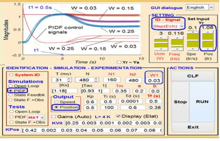
Figure 6 shows the screen view of
“GuiMexServoSys” tool, used to produce simulation
disturbance to be rejected by a robust PIDF feedback controller.
Figure 4. Experimental step response (with speed as output) and dynamic model identification from Strejc method
Figure 5. Graphs of an open loop input-delay servomechanism
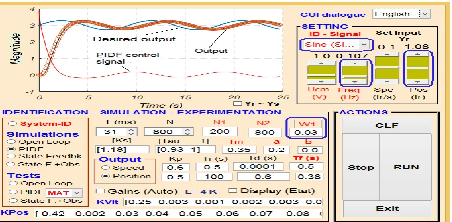
Figure 6. Step response simulation of PIDF-based feedback control servomechanisms
Figure 7. Simulation of precision and robustness of the PIDF-based control servo-system (step response)
Figure 6 shows the following conditions:
• No coupling effects (W = 0.0);
• The step control voltage is U = 1.2 V;
• In the absence of coupling effects, the robust PIDF feedback corrector is stable and follows the output reference.
In Figure 7, when the coupling effects intensify (W> 3% of the desired reference), the PIDF feedback controller loses robustness, and the dynamic input delay servo-system tends to move away from the desired output position. However, with a bounded amplitude of coupling effects (W<= 3% of the desired reference), the proposed PIDF controller remains very
reliable for its expected performance criteria, i.e., stability, fast response, zero static error, and robustness.
It is worth noting here that, in automatic control practice, a feedback controller with unbounded robustness margin is an utopic whish. What is important, however for the designer, is to be able to outline its robustness bounds for appropriate use.
Figure 8. Simulation of precision and robustness of the PIDF-based control servo-system (sine response)
In figure 8, the amplitude of the coupling effects is always at the limit value (W = 3% of the desired reference), and a sinusoidal waveform of adjustable frequency and amplitude, given by equation (12), is now applied as control signal on the testing platform.
ϴ(t) = ϴ0 + ϴm sin(2 πfpos t) (12) The results obtained when testing the precision and robustness of PIDF-based control servo-systems, are visualized in figure 8, where ϴ0 = 3 rad is a default offset term, ϴm being the magnitude to be adjusted from the scrolling bar Pos (position).
A relevant finding arising from figure 7 and figure 8, is that, under any disturbance W(t) with magnitude less than 3% of the desired reference, the proposed PIDF feedback control system for an input-delay robotic servomechanism, reaches the reference sine input at less than four seconds. In addition, during the whole steady operating regime, even permanent disturbances, it continuously offers very good precision and robustness qualities. It is possible to improve these qualities in the future version of “GuiServoSys” tool, equipped with embedded design strategies of optimal PIDF controllers.
CONCLUSION
This paper has presented original strategy and tools, for rapid modeling and simulation, of digital feedback
control of coupled input-delay servo-mechanisms. The simulation results emerging from prototyping coupled and uncertain servomechanisms, under digital PID controller, are very satisfactory. The error tracking and disturbance rejections levels, arising from simulation results, are reliable indicators of high precision and robustness, of the proposed digital PIDF-based feedback controller for input-delay robotic servo-mechanisms. In future research works, it will be fruitful to resort to optimal versions of digital PIDF controllers. Finally, the real time programming and embedding of the digital PIDF controller into a target
DSP chip, e.g. FPGA or SOC, will be very helpful, for real time testing the proposed decoupled PIDF-based feedback control architecture, on a real robotic system. CONTRIBUTION OF AUTHORS
Kom Charles Hubert, Associate Professor contributed to the revisions of the French version of the paper, provided by the main author. He also contributed to improve the literature review, and to translate the original French paper into English version paper. He formatted the final version of the paper to be submitted for reviewing, and then, continued to work as the corresponding author. He also evaluated and completed also revisions requested by the main author. Finally, he formatted and submitted for publication, the final expedited paper received from the supervisor of the research work, i.e., last co-author of the paper.
Mbihi Jean, Full Professor, contributed to the development of update of “GuiMexServoSys” tool, used to produce simulating results presented in this paper. He provided relevant guidelines for the synthesis of exact discrete model of input-delay transfer functions from their analog versions, using the m-order z-transform theory. He advised also the main author to use more beneficial PIDF controllers, compared to standard PID control strategies. He provided additional relevant answers, for a few relevant and valuable requests of two anonymous JEEECCS reviewers. In addition to the organization, supervision and revisions of common research works, he prepared and sent the last expertized and revised version of the paper, to the corresponding author, who was responsible to complete reformatting tasks, and to send the publishable version to JEEECCS.
Nomenclature
PIDF Proportional, derivative, integral with filter
SISO Single-input single-output
DSP Digital signal processing
FPGA Field Programmable Gate Array
e.g For example
DC Direct Current
i.e That is to say
MIMO Multiple-Input Multiple-Output
GUIMEX Servosyst
GUIde Matlab EXecutable Servo-systèm
Matlab GUI Matlab GUIde
SOC System On Chip
j Index variable
λj Time delay
Kj Static gain
τj Time constant
Uj, Yj Control input and output
respectively
ωj speed variable
ϴj Position variable
ϴ0 Default offset term for a sine
desired position
ϴm Magnitude of a sine desired
position can be adjusted
Wj Coupling disturbance (torque or
force)
Ej Tracking error
Pj Transfer function on the
disturbance
m Order of the modified
z-transform
N Default number of samples
Gωcj(s) Transfer function of the open loop decoupled dynamic model, with ω as output
Gcj(s) Transfer function of the open loop decoupled dynamic model, with ϴj as output
Dcj(s) Transfer function of the PIDF controller
Kpj Proportional gain
Kij Integral gain
Kdj Derivative gain
Tij Integral time constant
Tdj Derivative time constant
Tfj Filtered derivative time constant
Gj(z) Discrete transfer function of the decoupled dynamic model
Dj(z) Discrete transfer function of the PIDF controller
b0j, b1j , b2j , a0j and a1j
Variables resulting discrete transfer function of the PIDF controller calculated from Tustin method with a sampling period T
REFERENCES
[1] Y. Korem, “La robotique pour ingénieurss“, McGraw-Hiil edition, 342p., Newyork, 1986.
[2] C. Vibet, “Robotique – Principes et contrôle“, Ellipses Editions, 207 p., Prais, 1987.
[3] M. W. Spong, M. Vidyasagar, «Robot dynamic and control», John Wiley and sons, 336 p., Newyork.
[4] J. J. Crig, “Introduction to robotics – Mechanichs and control”, 2nd Edition, Addison Wesley Edition, 450 p. Newyorkk, 1989.
[5] B. Adrèa-Novel, “Commande no linéaire des robots“, Hermes editions, 312 p., Paris, 1989.
[6] S. Madanzadeh, A. Abedini, A. Radan, et J.-S. Ro, “Application of quadratic linearization state feedback control with hysteresis reference reformer to improve the dynamic response of interior permanent magnet synchronous motors“ , ISA Trans., sept. 2019.
[7] S. S. Ahmad et G. Narayanan, “Linearized Modeling of Switched Reluctance Motor for Closed-Loop Current Control“, IEEE Trans. Ind. Appl., vol. 52, no 4, p. 3146‑3158, juill. 2016.
[8] Y. Yan, J. Yang, Z. Sun, S. Li, et H. Yu, “Non-linear-disturbance-observer-enhanced MPC for motion control systems with multiple disturbances“, IET Control Theory Amp Appl., vol. 14, no 1, p. 63‑72, sept. 2019.
[9] G. Cheng, “Combined linear and non-linear controller design for motor position regulation“, Electron. Lett., vol. 54, no 5, p. 288‑289, janv. 2018.
[10] M. A. Asker, K. S. Gaeid, N. N. Tawfeeq, H. K. Zain, A. I. Kauther, et T. Q. Abdullah, “Design and Analysis of Robot PID Controller Using Digital Signal Processing Techniques“ , Int. J. Eng. Technol., vol. 7, no 4.37, p. 103–109, 2018. [11] M. S. Zaky, “A self-tuning PI controller for the speed control
of electrical motor drives“ , Electr. Power Syst. Res., vol. 119, p. 293‑303, févr. 2015.
[13] A. A. El-samahy et M. A. Shamseldin, “Brushless DC motor tracking control using self-tuning fuzzy PID control and model reference adaptive control“, Ain Shams Eng. J., vol. 9, no 3, p. 341‑352, sept. 2018.
[14] J. Mbihi, “Automatique analogique et techniques de commande et de régulation numérique”, ISTE Editions, 244 p., London, 2018.
[15] J. Mbihi, . “Analog Automation and digital feedback control techniques“, John Wiley and Sons Co-Edition, Newy Jersy, 2018.
[16] J. Mbihi, “A flexible multimedia workbench for digital control of input-delay servo systems“, J. Comput. Sci. Control Syst., vol. 8, no 2, p. 35, 2015.
[17] I. Klimo, P. Drahoš, et M. Kocúr, « PI controller implementation based on FPGA », in 2018 Cybernetics Informatics (K I), 2018, p. 1‑6.
[18] J. Mbihi, “Tchniques avancées et technologie de commande et régulation assistée par ordinateur”, ISTE Editions, 248 p. London, 2018.