Knots and Electromagnetism

a.j.j.m. d e k l e r k

K N O T S A N D E L E C T R O M A G N E T I S M

b a c h e l o r’s t h e s i s

s u p e r v i s e d b y

dr. R.I. van der Veen, dr. J.W. Dalhuisen, and prof. dr. D. Bouwmeester

2 5 j u n e 2 0 1 6

Mathematical Institute Leiden Institute of Physics

C O N T E N T S

1 i n t r o d u c t i o n 1

2 m i n k o w s k i s pa c e 3

2.1 The geometry of Minkowski space . . . 3

2.2 The Hodge star operator . . . 6

2.3 The Laplace-Beltrami operator . . . 11

3 e l e c t r o m a g n e t i s m 15 3.1 Maxwell’s equations . . . 15

3.2 Gauge freedom . . . 17

3.3 Self-duality . . . 19

3.4 The Bateman construction . . . 22

3.5 Superpotential theory . . . 23

4 k n o t s i n e l e c t r o m a g n e t i s m 25 4.1 Solenoidal vector fields . . . 25

4.2 The Hopf field . . . 27

4.3 Algebraic links . . . 29

4.4 Linked optical vortices . . . 35

5 c o n c l u s i o n 41

b i b l i o g r a p h y 43

1

Over the past decades, the interaction between knot theory and phys-ics has been of great interest. Both integral curves and zero sets that form knots, as well as invariants from knot theory, have arisen in physical theories. Particularly interesting is the occurrence of the Hopf fibration in many different areas of physics [22]. In

electromag-netism, the Hopf fibration arises as the field line structure of an elec-tromagnetic field, which we will refer to as the Hopf field. Its math-ematical elegance, and its physical relevance in relation to plasma physics were the main motivation for our research.

One of our initial goals was to derive the Hopf field in a way not relying on the topological model of electromagnetism by Ranada [17, 18], or the ad hoc choice of Bateman variables in [12]. Employing a

construction by Synge [21] allowed us to achieve this goal and gave

rise to Bateman variables for the Hopf field. Then, during a study of generalisations of the Hopf field proposed by Kedia et al. in [12],

we discovered a way of constructing electromagnetic fields such that the intersection of their zero set with an arbitrary spacelike slice in Minkowski space is a given algebraic link. These linked zero sets of electromagnetic fields in spacelike slices, also called optical vortices in physics, have already been studied both experimentally and theoretic-ally in [5,7,13]. The main difference between this previous work and

our result lies in the fact that our construction yields exact solutions to the Maxwell equations, while this prior work concerns paraxial fields. We should note that an exception is a paper by Bialynicki-Birula [6],

upon which we build.

This thesis starts with a study of Minkowski space and operators in-duced by its pseudo-Riemannian metric in chapter 2. Then we go on to formulate electromagnetism in terms of differential forms in chapter 3. Chapter 2 and 3 show how many well known and some less well known results from physics arise naturally from this math-ematical formalism. Furthermore, these chapters provide the neces-sary background for our treatment of the main results in chapter 4. In this chapter, we show how the Hopf field can be derived from a solution of the scalar wave equation. Finally, after a short digression on algebraic links, we show how self-dual electromagnetic fields can be derived such that its optical vortices are a given algebraic link.

2

In the absence of gravitational effects, Minkowski space is the appro-priate mathematical description of spacetime. It combines the spatial dimensions and time into a single four-dimensional whole with a non-Euclidian geometry. This geometry contains information about important physical concepts as we will see in section2.1. Apart from the study of Minkowski space itself, we will also study operators on Minkowski space in section2.2and section2.3. These operators will allow us to formulate electromagnetism in the formalism of differen-tial forms in chapter3.

2.1 t h e g e o m e t r y o f m i n k o w s k i s pa c e

An understanding of Minkowski space can help us understand elec-tromagnetism or any other theory of physics compatible with the special theory of relativity. Therefore we devote this section to a dis-cussion of the geometry of Minkowski space and its phyiscal inter-pretation.

d e f i n i t i o n 2.1.1: LetVbe ann-dimensional real vector space and

let gbe a bilinear form onV. Thengis said to be

• symmetric ifg(v,w) =g(w,v)for all v,w∈V.

• non-degenerateif g(v,w) =0 for all w∈ Vimplies thatv =0.

A symmetric non-degenerate bilinear form on a real vector space V is called a pseudo-Riemannian metric onV.

Note that a pseudo-Riemannian metric is very similar to a metric, only it need not be non-negative or satisfy the triangle inequality.

t h e o r e m 2.1.2: Let V be an n-dimensional real vector space and

let g be a pseudo-Riemannian metric onV. Then there exists a basis {e1, . . . ,en} for V such that g(ei,ej) = ±δij; such a basis is called orthonormal. Furthermore, the number of elements ej in different or-thonormal bases that satisfyg(ej,ej) =1 is the same.

Proof. See, for example, theorem1.1.1in [16].

The final property in theorem2.1.2allows us to unambiguously define the following property of pseudo-Riemannian metrics.

d e f i n i t i o n 2.1.3: Let V be ann-dimensional real vector space, let g be a pseudo-Riemannian metric on V, and let {e1, . . . ,en} be an orthonormal basis forV. Then the signature of gis a doublet of num-bers (p,q) where p and q are equal to the number of elements of {e1, . . . ,en}such thatg(ei,ei)is−1 and 1 respectively.

d e f i n i t i o n 2.1.4: Minkowski space M is a four-dimensional real

vector space endowed with a pseudo-Riemannian metric η of signa-ture (1, 3). An element v ∈ M is said to be timelike if η(v,v) < 0, lightlike ifη(v,v) =0, and spacelike ifη(v,v)>0.

To see how the geometrical structure of Minkowski space is consistent with our every day experience of three-dimensional space and time as seperate entities, we investigate special subspaces of Minkowski space.

d e f i n i t i o n 2.1.5: A linear subspace T ⊂ M is timelike if it is

spanned by a timelike vector t ∈ M. Furthermore, a linear subspace S ⊂ M is spacelike if it is the orthogonal complement of a timelike subspace.

Since the pseudo-Riemannian metric on Minkowski space restricted to a timelike subspace T of M is non-degenerate, we can conclude from proposition 8.18 in [20] that M = T⊕T⊥. Now, since _η has

signature (1, 3), we can conclude that T⊥ is spanned by three space-like vectors, so that the restriction of η to this subspace is Euclidian. Therefore, we would like to identify a spacelike subspace with our spatial dimensions, but there are infinitely many spacelike subspaces. This multitude of choices for a spatial dimension will turn out to be the mathematical equivalent of the principle of relativity. However, despite suggestive nomenclature, it remains unclear how the evolu-tion of time is incorporated in the geometry of Minkowski space. To this end we will consider more general subsets ofM.

d e f i n i t i o n 2.1.6: An affine subspace∑ofM is said to be a

space-like slice if it can be written as _∑ = t+S, where t ∈ M is timelike, andS=hti⊥is a spacelike subspace ofM.

Thus, given a fixed t ∈ M that is timelike, we get an orthogonal spacelike subspace S=hti⊥and we can write

M= G

λ∈R

λt+S

2.1 t h e g e o m e t r y o f m i n k o w s k i s pa c e 5

of this form remains. We will resolve this issue after studying the geometry of Minkowski space with respect to charts.

d e f i n i t i o n 2.1.7: A frame of reference is a chart (M,h,R4),

in-duced by a choice of basis {e0, . . . ,e3}forM, wherehis given by

h :M →R4, xµ_{eµ 7→(x}0_{, . . . ,x}3₎

Furthermore, we note thatxµ_e

µis supposed to denote the summation of xµ_{eµ over}

µfrom zero to three. The omission of summation signs is common practice in physics and is called the Einstein summation convention. It states that if an index appears both in an upper and a lower position, it should be summed over.

Note that theorem2.1.2implies that there exists an orthonormal basis {e0, . . . ,e3} for M, which we order such that η(e0,e0) = −1. Then,

any v,w ∈ M can be written asv = vµ_e

µ and w= wνeν andη(v,w) is given by

η(v,w) =−v0w0+v1w1+v2w2+v3w3

With respect to such a basis the matrix representation ofηis diagonal withη00=−1 andηii=1 for 1≤ i≤3. Thus, using the Einstein sum-mation convention, we may write η(v,w) = vµηµνwν. As is common in physcis textbooks, we will use greek letters to denote summation over all four coordinates of Minkowski space, and latin letters to de-note summation over x1,x2,x3.

d e f i n i t i o n 2.1.8: An inertial frame of reference is a chart on M

induced by an ordered orthonormal basis such that the first element of the basis e0 satisfiesη(e0,e0) =−1.

Note that choosing an ordered orthonormal basis (e0, . . . ,e3) such

that η(e0,e0) =−1, induces a splitting of Minkowski space by taking

the spacelike subspace to be spanned by e1,e2, and e3 and by taking

e0 as the timelike element in the splitting. Conversely, a splitting of

spacetime gives an orthonormal basis. To see this, note that we can take the timelike element of M in the splitting of spacetime to bee0,

and obtain three orthonormal basis vectors from the corresponding spacelike subspace Susing the Gram-Schmidt procedure.

d e f i n i t i o n 2.1.9: Let V be an n-dimensional real vector space

en-dowed with a pseudo-Riemannian metric g. Then a diffeomorphism f :V → V is called an isometry if g(f(v),f(w)) = g(v,w)holds for allv,w∈V.

p r o p o s i t i o n 2.1.1 0: Let V be an n-dimensional real vector space

endowed with a pseudo-Riemannian metric gand let f :V →V be a linear map. Then f is an isometry if and only if f maps orthonormal bases to orthonormal bases.

Proof. Let{e1, . . . ,en} be an orthonormal basis, and suppose f maps orthonormal bases to orthonormal bases. Then it follows that

g(f(ei), f(ej)) =g(e0i,e0j) =δij

Since f is linear andg is bilinear we can conclude from this that f is an isometry. Conversely, suppose that f is an isometry. Then we have

g(f(ei), f(ej)) =g(ei,ej) =δij

This shows that{f(e1), . . . ,f(en)}is orthonormal.

Thus different inertial frames and hence different splittings of Minkow-ski space, are related to each other by isometries. Choosing an iner-tial frame for Minkowski space is thought of in physics as putting an observer with a clock and a set of rulers somewhere in space. Differ-ent observers with consistDiffer-ently oriDiffer-ented directions of space and time are related to each other by Lorentz transformations that are posit-ive definite on the first component of any inertial frame and preserve the orientation on Minkowski space. The group of such transforma-tions is a subgroup of the Lorentz group called the restricted Lorentz group. In their classical form, the laws of physics are stated in terms of derivatives with respect to time and space as measured by such observers. However, we just discussed the ambiguity there is in this description. This problem is resolved by demanding that the laws of physics have the same ’form’ in different inertial frames, i.e. that the laws of physics are symmetric under the restricted Lorentz group. In the formalism of differential forms which we will employ throughout this thesis, this comes down to the following: if F is a solution of a physical law, and f : M → Mis an element of the restricted Lorentz group, then f∗(F)also has to be a solution of the equation. Often the laws of physics have more symmetry than required by this discussion, but we will not go into this deeply. For example, we will not determ-ine the most general groups under which an equation is symmetric, but if it is just as easy to prove that an equation is symmetric under the entire Lorentz group instead of just the restricted Lorentz group, we will show this instead.

2.2 t h e h o d g e s ta r o p e r at o r

2.2 t h e h o d g e s ta r o p e r at o r 7

operator. This operator will be necessary to formulate the wave equa-tion and Maxwell’s equaequa-tions in terms of differential forms.

p r o p o s i t i o n 2.2.1: Let V be an n-dimensional real vector space

and let g be a pseudo-Riemannian metric on V. Then the map T : V →V∗, v7→g(v, .)is an isomorphism.

Proof. BecauseV is finite dimensional we know that dimV =dimV∗ so that it is sufficient to show thatTis linear and injective. Letv,w∈ V andλ,µ∈R, then by bilinearity ofgwe have that

T(λv+µw) =g(λv+µw, .) =λg(v, .) +µg(w, .)

This shows thatTis linear. Now letv ∈Vand suppose thatT(v) =0, then it must hold for everyw ∈V that g(v,w) =0 which is the case if and only if v= 0 by the non-degeneracy ofg. This shows thatT is injective and concludes the proof.

This isomorphism betweenVandV∗induced by the pseudo-Riemannian metricgonV, induces a pseudo-Riemannian metric onΩ1(V). To see this, note that

h·|·i:Ω1(V)×Ω1(V)7→R, (ω,τ)7→ g(T−1(ω),T−1(τ)) satisfies the required properties. It can be shown that this induces a pseudo-Riemannian metric onΩk(V)by using the universal property of Λk(V∗) =Ωk(V).

l e m m a 2.2.2: Let V be an n-dimensional real vector space and let g be a pseudo-Riemannian metric on V. Then there is a pseudo-Riemannian metrich·|·ik_onΩk_{(V), such that for one-forms}

ω1, . . . ,ωk, τ1, . . . ,τk ∈ Ω1(V)we have

hω1∧ · · · ∧ωk|τ1∧ · · · ∧τkik =det[hωi,τji]

Proof. See, for example, lemma9.14as well as the remarks preceeding

and following it in [14].

t h e o r e m 2.2.3: Let V be an n-dimensional real vector space, let g

be a pseudo-Riemannian metric on V, and fix an orientation Vol ∈ Ωn_{(V). Then there is a unique linear map ? : Ω}k_{(V) → Ω}n−k_(V), called the Hodge star operator, such that for any ω,τ ∈ Ωk(V) it satisfies

ω∧?τ=hω,τik·Vol

Proof. See, for example, theorem9.22in [14].

concrete expression for the Hodge star operator. The following pro-position shows that for orthonormal bases such an explicit descrip-tion is particularly simple. Since we will only consider orthonormal bases, we will not require a more general explicit description.

p r o p o s i t i o n 2.2.4: LetVbe ann-dimensional real vector space

en-dowed with a pseudo-Riemannian metricgonVwith signature(p,q), and fix an orientation Vol∈Ωn_{(V). Furthermore, let(e}

1, . . . ,en)be an ordered orthonormal basis that is positively oriented, let (e1, . . . ,en)

be a corresponding ordered dual basis, and let{i1, . . . ,ik}and{ik+1, . . . ,in} be disjoint subsets of{1, . . . ,n}. Then we have

?(ei1 _{∧ · · · ∧e}ik_{) =±(−1)}p_eik+1_{∧ · · · ∧e}in

where we take the plus sign if ei1∧ · · · ∧_eik∧_eik+1 ∧ · · · ∧_ein _{is equal}

to the orientation onV, and the minus sign otherwise.

Proof. See, for example, proposition9.23in [14].

Proposition2.2.4allows us to easily see how the Hodge star operator acts on Minkowski space, and spacelike subspaces thereof.

e x a m p l e 2.2.5: First we choose an inertial frame and agree to

de-note the coordinate functions corresponding to our choice of ordered orthonormal basis (e0,e1,e2,e3)by(t,x,y,z). Then the natural

orient-ation onV corresponding to this choice of basis, is dt∧dx∧dy∧dz. Now we can apply proposition 2.2.4 to determine explicitly how the Hodge star acts on the basis for the differential forms induced by the coordinate functions. For the bases of the one-forms and three-forms induced by the chosen coordinate functions we get

?dt=−dx∧dy∧dz ?dx=−dy∧dz∧dt ?dy=−dz∧dx∧dt ?dz=−dx∧dy∧dt

?(dx∧dy∧dz) =−dt

?(dx∧dy∧dt) =−dz

?(dz∧dx∧dt) =−dy

?(dy∧dz∧dt) =−dx

Furthermore, the natural basis for the two-forms induced by our choice of coordinate functions satisfies

?(dx∧dt) =dy∧dz

?(dy∧dt) =dz∧dx

?(dz∧dt) =dx∧dy

?(dx∧dy) =−dz∧dt

?(dz∧dx) =−dy∧dt

?(dy∧dz) =−dx∧dt

Finally, the natural bases for the zero-forms and the four-forms satisfy

?1=−dt∧dx∧dy∧dz and ?(dt∧dx∧dy∧dz) =1

The spacelike subspaceSofMinduced by this choice of orthonormal basis is spanned by e1,e2, and e3. This subspace is naturally enowed

2.2 t h e h o d g e s ta r o p e r at o r 9

orientation to be dx∧dy∧dz. These choices induce a Hodge star operator onSwhich we will denote by?_S. This restricted Hodge star operator acts on the bases of one-forms and two-forms onSinduced by the coordinate functions as

?_Sdx=dy∧dz ?_Sdy=dz∧dx ?_Sdz=dx∧dy

?_S(dx∧dy) =dz ?_S(dz∧dx) =dy ?_S(dy∧dz) =dx

Finally, we have that

?S1=dx∧dy∧dz and ?_S(dx∧dy∧dz) =1

Furthermore, since Scan be viewed as a three-dimensional Euclidian space in its own right, there is an exterior derivative operator for forms on S which we will denote by dS. Since we will be working exclusively in Minkowski spacetime, this example allows us to com-pute the Hodge star of any differential form we will be interested in without having to refer to the abstract definitions.

In example2.2.5, we see that applying the Hodge star operator twice either gives the identity on Ωk(V) or the identity multiplied by a minus sign. This result turns out to be true in general, and whether we get a this extra minus sign or not, is determined by the signature of the metric as well as what type of form we start with.

p r o p o s i t i o n 2.2.6: Let V be an n-dimensional real vector space,

and let g be a pseudo-Riemannian metric onV with signature (p,q). Then for anyω∈ Ωk(V)it holds that

?2ω = (−1)p+k(n−k)ω

Proof. See, for example, proposition9.25in [14].

In particular, proposition 2.2.6 implies that the Hodge star operator is an isomorphism with inverse given by

?−1: Ωk(V)→Ωn−k(V), ω7→ (−1)p+k(n−k)?ω

It turns out that isometries not only play a special role with respect to the pseudo-Riemannian metric gthat Vis endowed with, but also with respect to the Hodge star operator through its dependence ong.

p r o p o s i t i o n 2.2.7: LetVbe ann-dimensional real vector space, let gbe a pseudo-Riemannian metric, and let f :V → Vbe an isometry. Then for anyω∈ Ωk(V)we have

f∗(?ω) =?f∗(ω) or f∗(?ω) =−? f∗(ω)

Proof. Let (e1, . . . ,en) be a positively oriented orthonormal basis for V with corresponding ordered dual basis(e1, . . . ,en). Then a basis of the forms is given by {ei1 ∧ · · · ∧_eik}_{if we let i}

1 through ik take on all possible values in{1, . . . ,n}. Therefore, it is sufficient to prove the proposition for forms of this type. Let f :V →Vbe an isometry, then it maps (e1, . . . ,en) to another orthonormal basis (f(e1), . . . ,f(en)) as shown in proposition 2.1.10. This new basis (f(e₁), . . . ,f(e_n)) is positively oriented if f is orientation preserving and negatively ori-ented otherwise. First we suppose that f is orientation preserving. Let{i1, . . . ,ik}and{ik+1, . . . ,in}be disjoint subsets of{1, . . . ,n}, then proposition2.2.4tells us that

f∗(?(ei1_{∧ · · · ∧e}ik_{)) = f}∗_(±(−1)p_eik+1∧ · · · ∧_ein₎

=±(−1)pf∗(eik+1_{)∧ · · · ∧ f}∗_(ein₎

=?(f∗(ei1_{)∧ · · · ∧ f}∗_(eik₎₎

=?f∗(ei1_{∧ · · · ∧e}ik₎

Herepdenotes the first component of the signature(p,q)ofg. Noting that we get an extra minus sign if f is orientation reversing because of the definition of the±1 in proposition2.2.4concludes the proof.

Having introduced the Hodge star operator, we are ready to formu-late the theory of electromagnetism in chapter3. However, as is often the case, things will simplify if we make the right definitions. There-fore we will first introduce two more operators, the codifferential op-erator in this section and the Laplace-Beltrami opop-erator in section2.3.

d e f i n i t i o n 2.2.8: LetVbe ann-dimensional real vector space and

let g be a pseudo-Riemannian metric on V. Then the codifferential operator is defined to be

δ :Ωk(V)→Ωk−1(V), ω 7→(−1)k?−1d?ω

Here the seemingly arbitrary factor of (−1)k is introduced so that δ is the adjoint of the induced pseudo-Riemannian metric we have on the space ofk-forms by proposition2.2.2.

p r o p o s i t i o n 2.2.9: LetVbe ann-dimensional real vector space, let gbe a pseudo-Riemannian metric, and let f :V →V be an isometry. Then for anyω∈ Ωk(V)we have f∗(δω) =δf∗(ω).

2.3 t h e l a p l a c e-b e lt r a m i o p e r at o r 11

time we interchange the pullback with respect to fand the Hodge star operator. Since the codifferential contains the Hodge star operator twice, these minus signs cancel.

As mentioned, we will formulate electromagnetism in terms of differ-ential forms in chapter3. However, we will do so in terms of complex-valued differential forms onMinstead of the real-valued differential forms discussed here. Therefore we note that in such cases we take the linear extension of the Hodge star operator to Ωk(M,C), i.e. the space of complex-valued differential k-forms. Furthermore, we note that all the results from this section are also valid for this linear ex-tension.

2.3 t h e l a p l a c e-b e lt r a m i o p e r at o r

In the previous section, we introduced the Hodge star operator and showed how it gave rise to the codifferential operator. There is a cer-tain combination of the codifferential operator and the exterior deriv-ative that we will encounter in this thesis. Therefore, we devote this section the study of this new operator called the Laplace-Beltrami op-erator, which on Minkowski spacetime acts as a generalisation of the wave equation for differential forms.

d e f i n i t i o n 2.3.1: LetVbe ann-dimensional real vector space and

let g be a pseudo-Riemannian metric. Then the Laplace-Beltrami op-erator is a linear map∆:Ωk_(V,C)→Ωk_{(V,C)given by∆=dδ+δd.} Before continuing, we will show that for zero-forms on Minkowski space the Laplace-Beltrami operator gives rise to the wave equation we are familiar with. LetW ∈ C∞(M,C), then we get

∆W = (dδ+δd)W = δdW = (−1)4?−1d?dW

because ?W is a four-form, and taking the exterior derivative gives a five-form which is zero on Minkowski space showing that δW = 0. Also, since?−1 is an isomorphism, it follows that∆W =0 if and only if d?dW=0. Calculatingd?dW explicitly gives

d?dW=d?(∂xWdx+∂yWdy+∂zWdz+∂tWdt)

=d(∂xWdy∧dz∧dt+∂yWdz∧dx∧dt

+∂zWdx∧dy∧dt+∂tWdx∧dy∧dz)

= (∂2_x+∂2_y+∂2_z−∂2_t)Wdx∧dy∧dz∧dt

e x a m p l e 2.3.2: Let ˜W :M →Cbe given by

˜

W(t,x,y,z) = (r2−t2)−1

where r2 = x2+y2+z2. Then we can check thatW is a solution of the wave equation, but it will have singularities. Therefore we shift the time variable by a constant imaginary factor, which we choose to be−i, givingW :M →Cgiven by

W(t,x,y,z) = (r2−(t−i)2)−1

Here the denominator is given by

r2−(t−i)2 =r2−t2+1−2it

Thus the imaginary part is zero if and only ift = 0, but in this case the real part reads r2+1 which is never zero, showing that W has no singularities. Now let us check that W is a solution to the wave equation. The first derivatives ofW are given by

∂tW =2(t−i)(r2−(t−i)2)−2 ∂xiW =−2xi(r

2_−(t−i)2₎−2

Here xi denotes x,y or z. The second derivatives can be found with the chain rule giving

∂2_tW =2(r2−(t−i)2)−2+8(t−i)2(r2−(t−i)2)−3

= (2r2+6(t−i)2)(r2−(t−i)2)−3

∂2_xiW =−2(r2−(t−i)2)−2+8x_i2(r2−(t−i)2)−3

= (−2(r2−(t−i)2) +8x2_i)

So we see that

∂2_xW+∂2_yW+∂2_zW = (−6(r2−(t−i)2) +8r2)(r2−(t−i)2)−3

= (2r2+6(t−i)2)(r2−(t−i)2)−3=∂2_tW

This shows thatW is indeed a solution of the wave equation.

Now let us return to our general discussion of the Laplace-Beltrami operator. Due to the symmetry in its definition, it behaves nicely with respect to the exterior derivative and the Hodge star operator as shown in the next proposition.

p r o p o s i t i o n 2.3.3: Let _ω ∈ Ωk(V,C), then the Laplace-Beltrami

operator satisfies∆dω= d∆ωand?∆ω =∆?ω.

Proof. Letω ∈ Ωk(V), where the symmetric non-degenerate bilinear form onVhas signature (p,q)and dimensionn, Then we have

∆dω = (dδ+δd)dω =dδdω

2.3 t h e l a p l a c e-b e lt r a m i o p e r at o r 13

becaused2_=0=δ2_{. Now we note that}

?δdω =?(−1)k+1?−1d?dω

= (−1)k+1+n−k+p+(k+1)(n−k−1)d(−1)n−k?−1d? ?−1ω

= (−1)k+1+n−k+p+(k+1)(n−k−1)dδ?−1ω

= (−1)k+1+n−k+p+(k+1)(n−k−1)+p+k(n−k)dδ?ω

=dδ?ω

Similarly we can prove that ?dδω = δd?ω. Combining these facts gives

?∆ω =?(dδ+δd)ω

=δd?ω+dδ?ω

=∆?ω This concludes the proof.

The final property of the Laplace-Beltrami operator we will need is the following.

p r o p o s i t i o n 2.3.4: Let A∈ Ω1(M,C)then we have that∆A=0 if

and only if the components of Awith respect to some basis satisfy the wave equation, i.e. if A= Aµdxµ _then∆_{A=0 if and only if}∆_Aµ=0 for all µ∈ {0, 1, 2, 3}.

3

In this chapter, we will formulate electromagnetism in the language of differential forms. Since we will be interested in electromagnetic fields in vacuum, we will not incorporate source terms in our treat-ment. Furthermore, we will not take into account any curvature of spacetime due to the energy density of the electromagnetic field as predicted by the general theory of relativity. Instead, we will assume that spacetime is modelled by Minkowski space as described in chapter 2. Finally, we note that parts of section3.1,3.2, and3.3 are based on [2] and exercises therein.

3.1 m a x w e l l’s e q uat i o n s

In electromagnetism, the objects of study are electric and magnetic fields, which were classically viewed as distinct time-dependent vec-tor fields onR3. However, it turned out that this description was less adequate in the context of special relativity because the electric and magnetic fields change according to the inertial frame of reference we choose. This observation indicated that the electric and magnetic fields are part of the same phenomenon called the electromagnetic field, which we will describe by smooth complex-valued two-forms on Minkowski space.

d e f i n i t i o n 3.1.1: A complex-valued two-form F ∈ Ω2(M,C) is

called an electromagnetic field if

dF=0 and δF=0

These equations are called the first and second Maxwell equation re-spectively. After choosing an inertial frame of reference for M, we can write

F= 1

2Fµνdx

µ_∧dxν _=E∧dt+B

provided that we define E = (Fi0−F0i)dxi and B = 1₂Fijdxi∧dxj. Furthermore, we defineEkandBkto be the complex-valued functions on M such that E = Ekdxk and ?SB = Bkdxk for any k ∈ {1, 2, 3}. From this we see that the real parts of E and B can be identified with vector fields on R3_{, which we will refer to as the electric and}

magnetic field respectively. We will denote the electric field by~Eand the magnetic field by~B.

With the choice forEand Bas in definition3.1.1, we can write down four equations forEandBequivalent to Maxwell’s equations. To find the first two of these equations, we plug F = E∧dt+B into the first Maxwell equations giving

0=dF=d(E∧dt+B) =dSE∧dt+∂tB∧dt+dSB

Thus we see that the first Maxwell equation corresponds to

dSE+∂tB=0 and dSB=0

Noting that δF = 0 is equivalent to d?F = 0 because ?−1 is an isomorphism, we plug F = E∧dt+Bintod?F. With example2.2.5, this can be seen to give

0=d(?_SE−?_SB∧dt)

=dS?SE+∂t?SE∧dt−dS(?SB)∧dt

Thus the second Maxwell equation corresponds to

∂t?SE−dS?SB=0 and dS?SE=0

These four equations for E and B to which Maxwell’s equations as defined in 3.1.1 are equivalent, are closer to the form in which one usually first encounters Maxwell’s equations. However, one of the several disadvantages of this formulation is that symmetry of Max-well’s equations under the restricted Lorentz group is not manifest.

p r o p o s i t i o n 3.1.2: Maxwell’s equations are symmetric under the

Lorentz group.

Proof. Let f : M → M be a diffeomorphism and let F ∈ Ω2_(M,C)

be an electromagnetic field. Then f∗(F)also solves the first Maxwell equation because the pullback commutes with the exterior derivative giving

d(f∗F) = f∗(dF) = f∗(0) =0

However, the second Maxwell equation is not invariant under general diffeomorphisms. Therefore we now assume f to be an isometry, in which case proposition2.2.9implies that

δf∗(F) = f∗(δF) = f∗(0) =0

This concludes the proof.

d e f i n i t i o n 3.1.3: Let F be an electromagnetic field and choose a

frame of reference givingEandBas in definition3.1.1. Then the field lines of the electromagnetic field are the integral curves of the vector fields corresponding to the real parts ofEandBinR3 at a fixed time.

3.2 g au g e f r e e d o m 17

r e m a r k 3.1.4: The first Maxwell equation states that an

electromag-netic field is in particular a closed complex-valued two-form. Since Minkowski space is a vector space, it follows that Hk(M,C) = 0 for any k ∈ _Z≥1. Therefore, there exists an A ∈ Ω1(M,C) such that

F=dA for any electromagnetic fieldF.

d e f i n i t i o n 3.1.5: Let F ∈ Ω2(M,C) be an electromagnetic field

and let A ∈ Ω1_{(M,C) be such that F = dA. Then A is called a}

potential forF.

It turns out that all the information of an electromagnetic field F is contained in a potential for F, and that we can write down an equa-tion for complex-valued one-forms that is equivalent to Maxwell’s equations.

p r o p o s i t i o n 3.1.6: LetF∈ Ω2(M,C), and letA∈ Ω1(M,C)such

that F=dA. ThenFis an electromagnetic field if and only ifδdA=0. If A∈Ω1_{(M,C)satisfiesδdA=0 we call it a potential.}

Proof. Suppose we have an electromagnetic field F ∈ Ω2_(M,C)and

let A∈ _Ω1_{(M,C)be a potential forF. PluggingF=dAin Maxwell’s}

equations gives

ddA=0 and δdA=0

This shows the implication from left to right. Conversely, let A ∈ Ω1_{(M,C)such thatδdA=0 and take F=dA. Then we get}

dF=ddA=0 and δF=δdA=0

This concludes the proof.

3.2 g au g e f r e e d o m

It turns out that an electromagnetic field does not correspond to a unique potential. This freedom in the choice of potential is called gauge freedom and can be used to make a potential satisfy additional conditions. When sufficient conditions have been imposed to remove any freedom in the choice of the potential, we say that the gauge has been fixed.

p r o p o s i t i o n 3.2.1: Let F ∈ Ω2(M,C)be an electromagnetic field,

let A ∈ _Ω1_{(M,C) be a potential for F, and let C ∈ Ω}1_(M,C).

Then A+C is a potential for F if and only if C = dc for some c∈ C∞(M,C).

Proof. LetF∈ Ω2_{(M,C)be an electromagnetic field, letA∈ Ω}1_(M,C)

be a potential for F, let C ∈ Ω1_{(M,C), and suppose A+C is also a}

potential forF. Then it must hold that

implying thatdC =0. SinceH1_{(M,C) =0, there exists ac∈C}∞_(M,C)

such that C = dc proving the implication from left to right. Con-versely, letc∈ C∞(M,C)and let A∈Ω1_{(M,C)be a potential for an}

electromagnetic field F∈ _Ω2_{(M,C). Then A+dc is a potential forF}

because we have

d(A+dc) =dA+ddc=dA= F

This concludes the proof.

Thus a potential for an electromagnetic field is only determined up to the addition of a closed complex-valued one-form. There are many additional conditions one can impose, but we will only make use of the Lorentz gauge which is defined as follows.

d e f i n i t i o n 3.2.2: Let A ∈ Ω1(M,C)then it is is said to be in the

Lorentz gauge ifδA=0.

In general, when a gauge is chosen in one inertial frame, it need not necessarily be satisfied in another. This is the case if the gauge con-dition is not symmetric under the restricted Lorentz group. However, the Lorentz gauge does have this property.

p r o p o s i t i o n 3.2.3: The Lorentz gauge condition is symmetric

un-der the Lorentz group.

Proof. Let f : M → M be an isometry, and let A ∈ _Ω1_{(M,C) be a}

potential in the Lorentz gauge. Then f∗(F)satisfies the Lorentz gauge because proposition2.2.9implies that

δf∗(A) = f∗(δA) = f∗(0) =0

This concludes the proof.

Even though a potential in the Lorentz gauge satisfies an additional condition, it does not fix the gauge entirely, i.e. there is still some freedom in the choice of potential. To see this, let A ∈ Ω1_{(M,C) be}

a potential in the Lorentz gauge and let c ∈ C∞(M,C) be a func-tion satisfying ∆c = 0. Then A+dc also satisfies the Lorentz gauge condition because of the remark following definition2.3.1we have

δ(A+dc) =δA+∆c=0=∆c=0

Thus A+dcand Acorrespond to the same electromagnetic field.

r e m a r k 3.2.4: Let A ∈ Ω1(M,C) and suppose that it satisfies the

Lorentz gauge condition. Then we know from proposition 3.1.6 that Ais a potential if and only if

δdA=0= (δd+dδ)A=∆A=0

3.3 s e l f-d ua l i t y 19

3.3 s e l f-d ua l i t y

In dimension four the Hodge star operator has the special property that it maps two-forms to two-forms. Furthermore, we know by pro-position 2.2.6 that for any F ∈ Ω2(M,C) we have that ?2F = −F. Thus as a linear operator on Ω2(M,C) the Hodge star operator has ±ias its eigenvalues.

d e f i n i t i o n 3.3.1: Let F ∈ Ω2(M,C)then it is is called self-dual if ?F=iFand anti-self-dual if?F= −iF.

Since we are ultimately interested in electromagnetic fields, we will use the conventions established in section3.1even though the complex-valued two-forms we consider in this section need not be electromag-netic fields unless stated otherwise. Thus we write anyF∈ Ω2_(M,C)

as F = E∧dt+B where E and B are defined as in 3.1.1. Now the Hodge dual of F is given by ?F = ?_SE−?_SB∧dt. Thus we see that F is self-dual if and only if?_SB = −iE and anti-self-dual if and only if ?_SB = iE. More explicitly, F is self-dual if and only if Bk = −iEk and anti-self-dual if and only if B_k = iE_k for allk ∈ {1, 2, 3}. Further-more, we note that if F ∈ Ω2_{(M,C) is a self-dual or anti-self-dual}

complex-valued two-form that solves the first Maxwell equation, it also automatically satisfies the second Maxwell equation.

p r o p o s i t i o n 3.3.2: Let F ∈ Ω2(M,C), then we can write F as a

sum of self-dual and anti-self-dual two-forms F+ andF− respectively.

Proof. LetF ∈Ω2_{(M,C)and define}

F−= 1

2(F+i?F) and F+= 1

2(F−i?F)

Note that

?F+= 1

2(?F+iF) = i

2(F−i?F) =iF+ as well as

?F−= 1

2(?F−iF) =− i

2(F+i?F) =−iF−

This shows that F+ is self-dual and F− is anti-self-dual. Noting that

F= F++F−concludes the proof.

Proposition 3.3.2 implies that, in principle, it is sufficient to consider self-dual and anti-self-dual electromagnetic fields since any solution can be written as a sum of such fields.

p r o p o s i t i o n 3.3.3: Let F ∈ Ω2(M,C)and consider the parity

in-version map P : M → M, (t,x,y,z) 7→ (t,−x,−y,−z). Then P∗(F)

Proof. Note that pullback by a parity transformation leaves differen-tial forms of the form dxi ∧dxj unchanged, and flips the sign of differential forms of the form dxi ∧dx0. Therefore, the the compon-ents of E gain a minus sign with respect to the components of B after pullback by a parity transformation. This observation, combined with the proof below definition3.3.1that F is self-dual if and only if B_k = iE_k and anti-self-dual if and only if B_k = −iE_k, proves the pro-position.

The dimension of Ω2(M,C) is six, and by the previous proposition we know thatP∗ maps from self-dual elements of Ω2(M,C)to anti-self-dual elements ofΩ2(M,C). Furthermore, we know that

id_Ω2_(M,C) = (P◦P)∗ =P∗◦P∗

showing that P∗ is a bijection. This observation, combined with the result from proposition 3.3.2 that any element of Ω2(M,C) can be written as a sum of self-dual and anti-self-dual two-forms, shows that the dimension of the subspace of self-dual two-forms in Minkowski spacetime is three just like the dimension of the subspace of anti-self-dual two-forms.

For the remainder of this thesis we will only consider self-dual forms because we can obtain the corresponding anti-self-dual two-form by pullback with the parity inversion map. Furthermore, all the results we derive for self-dual electromagnetic fields in this section, also hold for anti-self-dual fields with similar proofs.

d e f i n i t i o n 3.3.4: Let F ∈ Ω2(M,C) be an electromagnetic field,

then the invariants of Fare?(F∧F)and?(F∧?F).

Taking an orthonormal basis for M and writing F = E∧dt+B as introduced in definition 3.1.1 allows us to rewrite the fundamental invariants of Fin terms of the components ofEandB. Then?(F∧F)

is given by

?(F∧F) =−2(ExBx+EyBy+EzBz)

and?(F∧?F)is given by

?(F∧?F) =−(E2_x+E2_y+E2_z−B2_x−B2_y−B_z2)

Furthermore, it turns out that

?(?F∧?F) =?(F∧F)

3.3 s e l f-d ua l i t y 21

pullback with respect to such a map commutes with the Hodge star operator, so that we get

f∗(?(F∧F)) =?[f∗(F∧F)] =?[(f∗F)∧(f∗F)]

as well as

f∗(?[F∧?F]) =?[f∗(F∧?F)] =?[(f∗F)∧(f∗?F)]

It turns out that the invariants of an electromagnetic field Fvanish if Fis self-dual.

p r o p o s i t i o n 3.3.5: Let F ∈ Ω2(M,C) be a self-dual

electromag-netic field then the fundamental invariants ofF vanish.

Proof. LetF∈_Ω2_{(M,C)be a self-dual electromagnetic field, then we}

have

?(F∧F) =?(?F∧?F) =?(iF∧iF) =−?(F∧F)

This shows that?(F∧F) =0, but we also have

?(F∧?F) =i?(F∧F) =0

Thus both the fundamental invariants of a self-dual electromagnetic field are zero.

As a consequence, the electric and magnetic field corresponding to self-dual electromagnetic fields are orthogonal. To see this, note that

?(F∧?F) =Re[Ex]2−Im[Ex]2+2iRe[Ex]Im[Ex] +. . .

Here we did not write down the similar terms we get for the y and z components of Eand the components of B. Due to self-duality we know that for anyk∈ {x,y,z}we haveBk =−iEkwhich implies that

Im[E_k] =Re[B_k]

Combining this with the fact that?(F∧?F) =0 gives

Re[Ex]Re[Bx] +Re[Ey]Re[By] +Re[Ez]Re[Bz] =0

i.e. ~E·~_{B = 0. We know that} ~_{E and} ~_{B depend on the inertial frame} chosen. However, we only used the Lorentz-invariant expression?(F∧ ?F) =0, and the self-duality condition to show that~E·~B =0. There-fore we can conclude that this holds regardless of the inertial frame we choose. As a consequence of this, [10] implies that a self-dual

3.4 t h e b at e m a n c o n s t r u c t i o n

In this section we will discuss a method of constructing self-dual elec-tromagnetic fields that is commonly referred to as the Bateman con-struction since it is originally due to Bateman [4]. This construction

will be essential to our method of constructing self-dual electromag-netic fields with linked optical vortices.

Let α,β : M → C be two smooth complex functions on Minkowski space, then F :=dα∧dβis a closed two-form onM. Hence it solves the first Maxwell equation. Note that F also solves the second Max-well equation if F is self-dual. Writing out the self-duality condition ?F = iFfor F = dα∧dβ gives that the self-duality condition is equi-valent to the Bateman condition forαandβ:

∇α× ∇β=i(∂tα∇β−∂tβ∇α)

Though this construction gives a different way of obtaining electro-magnetic fields, we must admit that to use it we still have to solve a difficult equation. However, once we have found solutions to these equations, we have the freedom to construct a whole family of other self-dual solutions as explained in the next proposition.

p r o p o s i t i o n 3.4.1: Let _α,_β: M → Cbe smooth functions

satisfy-ing the Bateman condition and let f,g :C2 →Cbe arbitrary smooth functions. ThenF =d f(α,β)∧dg(α,β)is a self-dual electromagnetic field.

Proof. Let α,β ∈ C∞(M,C) such that dα∧dβ is a self-dual electro-magnetic field, and let f,g : C2 _{→ C be smooth. Then d f(α,β)∧}

dg(α,β)is a closed two-form on Mthat can be written as

d f(α,β)∧dg(α,β) = (∂αf dα+∂βf dβ)∧(∂αgdα+∂βgdβ)

=∂αf∂βgdα∧dβ+∂βf∂αgdβ∧dα

= (∂αf∂βg−∂βf∂αg)dα∧dβ

Sincedα∧dβis self-dual we also know that

?d f(α,β)∧dg(α,β) =?(∂αf∂βg−∂βf∂αg)dα∧dβ

= (∂αf∂βg−∂βf∂αg)?(dα∧dβ)

= (∂αf∂βg−∂βf∂αg)idα∧dβ

=id f(α,β)∧dg(α,β)

Thusd f(α,β)∧dg(α,β)is also a self-dual electromagnetic field.

3.5 s u p e r p o t e n t i a l t h e o r y 23

t h e o r e m 3.4.2: Let F ∈ Ω2(M,C) be a self-dual electromagnetic

field, then there are α,β : M → Csatisfying the Bateman condition such that F=dα∧dβholds.

Proof. This result is due to Hogan who showed it, albeit using a dif-ferent formalism, in [9].

3.5 s u p e r p o t e n t i a l t h e o r y

It turns out that one can obtain solutions to the Maxwell equations by combining solutions to the wave equation with constant two-forms. Our treatment of this method in this section is based on the approach taken by Synge in section 13of chapter 9of [21], although he uses a

different formalism.

p r o p o s i t i o n 3.5.1: LetK∈Ω2(M,C)be a constant two-form and

let W ∈ _C∞(M,_C) be a solution of the wave equation. Then A =

?(dW∧K)is a potential, i.e.F=dAis an electromagnetic field.

Proof. First note that Ais in the Lorentz gauge because

δA=δ?(dW∧K) =?−1d? ?(dW∧K) =?−1dd(WK) =0

by proposition 2.2.6 and the fact that d2 = 0. Now we know from section3.2that Ais a potential if and only if∆A=0.

∆A=∆?d(WK) =?d∆(WK)

Here we could swap ∆with das well as?by proposition2.3.3. Now note that ∆(WK) = 0 if and only if the components of WK satisfy the wave equation by proposition2.3.4. This condition is satisfied be-cause W satisfies the wave equation andK has constant components concluding the proof.

Because of the special properties of self-dual electromagnetic fields, we would like to know when the electromagnetic fields correspond-ing to potentials as constructed in3.5.1are self-dual. It turns out that if we write out?d?(dW∧K) =id?(dW∧K)respectively?d?(dW∧ K) =−id?(dW∧K), we find thatKhas to satisfy

Kxy =−iKzt, Kzx=−iKyt, Kyz= iKxt

in the self-dual case and

Kxy =iKzt, Kzx=iKyt, Kyz=−iKxt

4

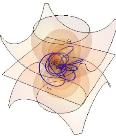
The purpose of this chapter is to derive the Hopf field, and to show how knot theory can be implemented in electromagnetism. To this end, we will first review the main result from the bachelor thesis of Ruud van Asseldonk [1] in section 4.1. We will then use the results from this section to show how the Hopf field can be obtained from the construction discussed in section 3.5. Finally, after a digression on algebraic links, we will arrive at the main result of this thesis in section4.4. Here, we will give a constructive proof that self-dual elec-tromagnetic fields exist with the special property that the intersection of their zero set with an arbitrary spacelike slice in Minkowski space is a given algebraic link.

4.1 s o l e n o i d a l v e c t o r f i e l d s

In this section we will discuss a method of constructing solenoidal vector fields onR3, i.e. vector fields~B:R3→R3_{that satisfy∇ ·~B=}

0. Furthermore, we will show how this construction can be used to derive a vector field with the property that its integral curves are all linked circles. However, as we did throughout this thesis, we will work with differential forms instead of vector fields. Therefore we note that solenoidal vector fields correspond to two-forms B ∈ Ω2_(R3_{) that satisfy dB = 0, or one-forms E ∈ Ω}1_(R3_{) that satisfy}

d?_SE = 0. The treatment we present in this section is based on sec-tion4.3of [1], the bachelor thesis of Ruud van Asseldonk.

r e m a r k 4.1.1: From the discussion following definition 3.1.1, we know that a magnetic field is a solenoidal vector field, but to get a solution to Maxwell’s equations we also need a solenoidal electric field that is coupled to the magnetic field in the correct way. Since the construction we will discuss in this section gives only one solenoidal field, it is not a method of constructing electromagnetic fields. The reason we decided to include this section is that it does give a good handle on the structure of the field lines, which will prove useful in section4.2.

r e m a r k 4.1.2: Let Nbe a two-dimensional manifold, then any_ω∈

Ω2_{(N)is closed. Now let f :R}3 _{→Nbe a smooth map, then f}∗₍

ω)is

a closed form onR3_{, because the pullback and the exterior derivative}

commute, i.e.

d f∗(ω) = f∗(dω) = f∗(0) =0

Thus this gives a method of constructing closed two-forms on R3_.

This remark in itself is rather trivial, but it turns out to be interesting because the fibre structure of f is closely related to the structure of the field lines as shown by theorem4.1.3.

t h e o r e m 4.1.3: Let N be a two-dimensional smooth manifold, let ω∈ Ω2(N), and let f :R3 → Nbe a smooth map. Then the fibres of f coincide with the field lines of f∗(ω)where the latter is non-zero.

Proof. Let N be a two-dimensional manifold, let f : R3 _{→ N be a}

smooth map, and letω∈ Ω2(N). Let(U,h,R2)be some chart, where h:U→R2_{is given by p7→(q}1_,q2_{). Then we can write}

ω|U = ωU·dq1∧dq2

for some ωU ∈ C∞(U). Now, on f−1(U), which is open because f is smooth, so in particular continuous, f∗(ω)is given by

f∗(ω|U) = (ωU◦f)·d f1∧d f2

The vector field on V corresponding to this form on V is given by

(ωU ◦ f)∇f1× ∇f2. Unless this vector field is zero at some point, which corresponds to f∗(ω)being zero on this point, the vector field is orthogonal to the integral curves of f. To see this, note that the gradients of f1 _{and f}2 _{are orthogonal to the level curves of f, so the}

outer product of these gradients at a point will be a tangent vector of the level curve of f through this point provided that this outer product is non-zero. Thus the integral curves of the vector field cor-responding to the form f∗(ω) correspond to the level curves of f where the former is non-zero.

There are many possibilities for the two-manifold N and the map f : R3 → N in theorem4.1.3. However, we will restrict our attention to the specific case whereN =S2_{, and the map f :R}3 _→S2_{is derived}

from a map called the Hopf map. The Hopf map is the restriction of ˜

H:C2→P1_{(C), (z}

1,z2)7→ (z1 :z2)

to S3 viewed as the subset of C2 of unit norm. Since we can identify

P1_{(C)with S}2_{, we can view this as a map fromS}3 _toS2_{. Composing}

the Hopf map with the inverse stereographic projection from R3 to

S2_{, gives the map}

φ:R3 →S2,     x y z     7→      

4(y(x2_+z2_{−1)−2xz+y}3₎

(x2_+y2_+z2₊₁₎2

−4(z(x2+y2−1)+2xy+z3)

(x2_+y2_+z2₊₁₎2 8(x2+1)

(x2_+y2_+z2₊₁₎2 − 8

x2_+y2_+z2₊₁+1

4.2 t h e h o p f f i e l d 27

The fibres of this map are circles which are all linked with each other. We will formally introduce linking in definition 4.3.4, the intuitive notion of linking should suffice for now. However, there is also one fibre that is not a circle, but a straight line. For more details on this map and its fibre structure see chapter3of [1]. Note that forms onS2

can be viewed as forms on R3. If we do this, one of the orientation forms onS2_{is given by}

ω= xdy∧dz+ydz∧dx+zdx∧dy

Taking the pullback ofω withφgives

φ∗(ω) =− 32(xz+y)

(x2_+y2_+z2₊₁₎3dx∧dy

− 32(xy−z)

(x2_+y2_+z2₊₁₎3dz∧dx

− 16 x

2_−y2_−z2₊₁

(x2_+y2_+z2₊₁₎3 dy∧dz

Though we have taken the same approach as in [1], we end up with a

form that differs by a minus sign and a transformationx 7→ −x. This difference is due to the choice we made in identifyingR4 _withC2_.

4.2 t h e h o p f f i e l d

The Hopf field is a self-dual electromagnetic field such that at t = 0 the field lines of both the electric and the magnetic field have the structure of the Hopf fibration, and are mutually orthogonal. In this section, we will show a new way of constructing the Hopf field using the method discussed in section3.5.

To obtain an electromagnetic field from the construction in section 3.5, we need a solution to the wave equation. We take this to be the solution without singularities found in example2.3.2, i.e.

W(t,x,y,z) = (x2+y2+z2−(t−i)2)−1

The construction also requires aK ∈ _Ω2_{(M,C) with constant}

coeffi-cients, which we choose to be

K =−dz∧dx−i·dy∧dz−dx∧dt+i·dy∧dt

Fur-thermore, proposition 3.5.1 guarantees that A = ?(dW∧K)is a po-tential, which is given by

A= −2(y+ix)

(x2_+y2_+z2_−(t−i)2₎2dz+

2(y+ix)

(x2_+y2_+z2_−(t−i)2₎2dt

+ −2it+2iz−2

(x2_+y2_+z2_−(t−i)2₎2dx+

−2t+2z+2i

(x2_+y2_+z2_−(t−i)2₎2dy

Now the electromagnetic field corresponding to Ais

F= 4(t−x+iy−z−i)(t+x−i(y+1)−z)

(x2_+y2_+z2_−(t−i)2₎3 dy∧dz

−4i(t−ix−y−z−i)(t+ix+y−z−i)

(x2_+y2_+z2_−(t−i)2₎3 dz∧dx

− 8i(t−z−i)(y+ix)

(x2_+y2_+z2_−(t−i)2₎3dx∧dy+. . .

Here we did not write down the terms determining the electric field, because they are fixed by self-duality when the terms determining the magnetic field are given. Note that at t = 0 we have 4Re[B] =

φ∗(ω), where φ∗(ω) is the two-form we determined in section 4.1. This shows that the field lines of the magnetic field have the same structure as the field lines of the vector field corresponding toφ∗(ω), which is that of the Hopf fibration. The same holds for the electric field by self-duality, which also implies that the field line structure is preserved in time due to the final result of section3.3. We would now like to determine Bateman variables for this electromagnetic field, i.e. maps ˜α, ˜β : M → C such that F = dα˜ ∧dβ˜. Note that for such a field, a potential is given by A = αd˜ β˜ = −βd˜ α˜, so we might hope to obtain Bateman variables for the Hopf field from the potential. If we compare the components of the potential, we see that two of them differ by a minus sign, and the other two differ by a factor of i. Thus, this gives us two natural choices to take for ˜α, ˜β, but these can never be Bateman variables for the field since it would give a field with a factor (r2_−(t−i)2₎−4_{. Therefore, we take the components without}

the square in the denominator, i.e.

˜

α(t,x,y,z) = 2i−2t+2z

r2_−(t−i)2 and β˜(t,x,y,z) =

2(ix+y)

r2_−(t−i)2

It turns out that these do, indeed, function as Bateman variables for the Hopf field, but we have some freedom here. We can take a factor ofifrom ˜αto ˜βand add 1 toiα˜ without changing the field. This gives new Bateman variables given by

α(t,x,y,z) = r

2_−t2_−1+2iz

r2_−(t−i)2 and β(t,x,y,z) =

2(x−iy)

r2_−(t−i)2

These are the form of Bateman variables used in [12], and will form

4.3 a l g e b r a i c l i n k s 29

4.3 a l g e b r a i c l i n k s

In this section, we will give a short exposition on algebraic link the-ory. We will only cover parts of the theory that are relevant for our construction in section4.4. More information can be found in the ref-erences used to write this section, which are [3,8,15,19,23].

d e f i n i t i o n 4.3.1: A link is a pair (X,L), where X is an oriented

manifold diffeomorphic toR3_{, andLis an one-dimensional}

submani-fold of Xdiffeomorphic to tn

i=1S1for somen∈Z≥1 with the

orienta-tion induced by the standard orientaorienta-tion onS1. Ifn=1, a link is said to be a knot.

We should note that whenever we refer to the main result of section 4.4, we identify links with one-dimensional manifolds diffeomorphic to tn

i=1S1 for somen∈ Z≥1. This is done for brevity, but in all

theor-ems, propositions, and proofs we will use the precise definition of a link stated above.

d e f i n i t i o n 4.3.2: Two links(X,L)and(X0,L0)are said to be

equi-valent if there exists an orientation preserving diffeomorphism ϕ : X→Xsuch that ϕ(L) =L0, and such thatϕ∗(ω) =ω0, whereω and ω0 are the orientations onLand L0 respectively. Two equivalent links are denoted by(X,L)∼= (X0,L0).

In section 4.2, we encountered the concept of linking in our brief description of the Hopf fibration. Even though, intuitively, it is clear what is meant by this, we will now formally define the notion of linking. To do so, we need the notion of a Seifert surface.

t h e o r e m 4.3.3: Let (X,K) be a knot, then there is a compact,

two-dimensional orientable submanfold S of X, such that ∂S = K. We take S to have the orientation induced by the orientation on K. Such a surfaceSis called a Seifert surface for the knot (X,K).

Proof. See chapter5in [19]

Even though there can be multiple Seifert surfaces for a given knot, it can be used to unambiguously define the linking number of two knots as we will now show.

d e f i n i t i o n 4.3.4: Let (X,K) and (X,K0) be knots such that K0∩ K = ∅, and let S be a Seifert surface for K. We may assume that S intersects K0 transversely in finitely many points, because if it does not we can deform its interior until it does. Let ϕ : X → R3 be a diffeomorphism betweenXandR3, and letωbe the orientation onX induced by the standard orientation on R3. Now, let p ∈ K0∩S, and take v1,v2 ∈ TpSsuch that ϕ∗(v1), andϕ∗(v2)are right-handed with

that ω0(w)>0 for the orientationω onS1. Finally, we defineσ(p)to be equal to one if ω(v1,v2,w) > 0, and to be equal to −1 otherwise.

Then the linking number of the knots is defined to be

L(K,K0) =

∑

p∈K0_∩S

σ(p)

Note that this definition is independent of the chosen Seifert surface for K. To see this, let S0 be another Seifert surface for K, and reverse the orientation on S0. Then S∪S0 is a closed surface in X, and hence for any p ∈ K0∩(S∪S0) such that σ(p) = 1, there is another p0 ∈ K0∩(S∪S0)such thatσ(p0) =−1.

In section 4.4, we will show how we can implement a certain class of links in electromagnetism. Therefore we will restrict our attention to this subclass, called the algebraic links. However, before being able to say what makes a link algebraic, we need the notion of a plane curve.

d e f i n i t i o n 4.3.5: A complex plane curve is the zero set of a

poly-nomial h ∈ C[v,w] viewed as a map h : C2 → C, (v,w) 7→ h(v,w)

that satisfies h(0, 0) = 0 and has an isolated singularity or a simple point in the origin. We will always work inC2_{, so we will simply refer}

to such a zero set as a plane curve.

Note thatC[v,w]is a unique factorisation domain, i.e. anyh∈ C[v,w]

can be written as a product of irreducible elements and a unit in

C[v,w]. Furthermore, this factorisation is unique up to ordering of the irreducible factors and multiplication of the irreducible factors by unit elements.

d e f i n i t i o n 4.3.6: LetCbe a plane curve associated to ah∈ C[v,w],

then a branch ofCis the zero set of an irreducible factor ofh.

Now we are ready to define algebraic links, but before we do so, we should say that we will denote the three-sphere of normeinC2byS3_e. Furthermore, we note that for anyp ∈S3_{the stereographic projection}

gives a diffeomorphism betweenS3_e\{p}andR3.

d e f i n i t i o n 4.3.7: A link(X,L)is said to be algebraic if there exists

a plane curveC, ane∈R>0, and ap∈S3e\Csuch that

(X,L)∼= (S_e3\{p},C∩S3_e)

r e m a r k 4.3.8: Instead of describing an algebraic link as the

inter-section of a plane curve C with a sphereS3

e, it can also be described by the intersection of a plane curve with

∂(D2(e)×D2(δ)) ={(v,w)∈C2||v|=e,|w| ≤δ or|v| ≤e,|w|=δ} Here e and δ can be chosen such that the square sphere intersects withCin a solid torus, where |x|=e. This alternative description of algebraic links was proposed by Kähler in [11] and will prove useful

4.3 a l g e b r a i c l i n k s 31

It turns out that every polynomialh ∈_C[v,w]that satisfiesh(0, 0) =0 and has an isolated singularity or a simple point in the origin gives rise to a link.

p r o p o s i t i o n 4.3.9: Let h ∈ C[v,w]such that h(0, 0) =0 and such

that h has an isolated singularity or a simple point in the origin and let C denote the plane curve corresponding to h. Then there is an e∈R>0and a p∈S3e such that(S

3

e\{p},C∩S

3

e)is a link. Such a link is algebraic by construction.

Proof. See lemma5.2.1and the remarks following it in [23].

Theein the definition of an algebraic link is necessary because there may be other singularities in the plane. The idea is to choose esmall enough such that S3_e does not enclose any singularity outside of the origin. However, this still leaves a range of choices for e, but we will now see that all values in this range give equivalent links.

l e m m a 4.3.1 0: Let C be a plane curve, then for _e,_e0 ∈ R_>0 small

enough, there are p∈S3

e andp

0 _∈S3

e0 such that

(S3_e\{p},C∩_S3

e)∼= (S

3

e0\{p

0_},C∩S3

e0) Proof. See, for example, lemma5.2.2in [23].

Having discussed how algebraic links arise from zero sets of polyno-mials, we will now elaborate on how a polynomial determines the topology of the algebraic link it induces.

p r o p o s i t i o n 4.3.1 1: Let (X,L) be an algebraic link induced by a

plane curve C corresponding to a polynomial h ∈ C[v,w]. Then the number of connected components ofLis equal to the number of irre-ducible factors into whichhcan be decomposed.

Proof. See the paragraph following lemma5.2.1in [23].

It turns out that every component of an algebraic link is completely determined by a corresponding irreducible factor of the polynomial that induces it; see section 2.3 in [23]. Therefore, we will restrict our

treatment to knots corresponding to irreducible polynomials. To say more about the topology of the knot that an irreducible polynomial h ∈ _C[v,w] induces, we will solve h(v,w) = 0 for w in terms of v. That such a solution can be obtained is a result due to Newton, and convergence of the solution forwwas later shown by Puiseux’.

t h e o r e m 4.3.1 2: Let h ∈ C[v,w] such that h(0, 0) = 0, then the

Proof. See, for example, theorem2.2.1and section2.2in [23].

The proof to theorem4.3.12gives successive approximations forwin terms of vof the form

w0= a0v

p0

q0

w1= v

p0

q0_(a 0+a1v

p1

q1₎

.. .

Such an expression for w in terms of fractional powers of v will be reffered to as a Newton expansion. The corresponding Puiseux’ ex-pansion is then obtained by takingv=tnand substituting it into the expansion for w. Herenis chosen to be equal ton=q0·q1· · · which

is finite as shown in the proof. Thus, such a solution is characterised by the exponents, determined by (pi,qi)in the successive approxim-ations. We can take these pairs to be coprime, and we will refer to them as the Newton pairs.

We will now give a description of the topology of a knot based on the Newton pairs and remark 4.3.8. Before doing so, we note that a knot (X,K) is equivalent to the embedding ιK : K → X of K in X. This description of a knot is better suited to describe the topology of a knot, so we will use it for now. First consider the simplest case, where there is only one Newton pair (p,q), where we take p and q to be coprime as noted before. Then the corresponding Newton expansion isw=vp/q_{, and substitutingv=ee}iθq_givesw=

ep/qeiθp/q. With these choices forv andw, we have a parametrisation (v,w) of the knot that lies on a torus. As v goes around the circle of radius eonce,v goes p/qtimes around the circle of radius ep/q. The curve

(eeiθq_,

ep/qeiθp/q) describing the knot, closes after v has gone around the toroidal direction of the torus ptimes, andwhas gone around the toroidal direction of the torus q times. Such a knot is called a (p,q)

torus knot. To deal with the more general situation with more than one Newton pair, we need the concept of a cable knot.

d e f i n i t i o n 4.3.1 3: Let (X,K) be a knot with corresponding

em-bedding ιK. Then a tubular neighbourhood ofιK is an embedding of the solid torus τ : S1×D2 → X in X such that τ(t, 0) = ι(t) for all t∈S1_.

It turns out that such a tubular neighbourhood always exists, but it is not unique. To see this, note that given a tubular neighbourhoodτof a knotιK, we can obtain another as follows. Define

ϕt :S1×D2→S1×D2, (s,d)7→(s,std)