AN M DWARF COMPANION TO AN F-TYPE STAR IN A YOUNG MAIN-SEQUENCE BINARY
Ph. Eigmüller1,2, J. Eislöffel2, Sz. Csizmadia1, H. Lehmann2, A. Erikson1, M. Fridlund1,3,4, M. Hartmann2, A. Hatzes2, Th. Pasternacki1, H. Rauer1,5, A. Tkachenko6,8, and H. Voss7
1
Institute of Planetary Research, German Aerospace Center Rutherfordstr. 2, D-12489 Berlin, Germany;[email protected]
2
Thüringer Landessternwarte Tautenburg Sternwarte 5, D-07778 Tautenburg, Germany 3
Leiden Observatory, University of Leiden P.O. Box 9513, 2300 RA, Leiden, The Netherlands 4
Department of Earth and Space Sciences, Chalmers University of Technology, Onsala Space Observatory, SE-439 92, Onsala, Sweden 5
Department of Astronomy and Astrophysics, Berlin University of Technology, Hardenbergstr. 36, D-10623, Berlin, Germany 6
Instituut voor Sterrenkunde, KU Leuven Celestijnenlaan 200D, 3001 Leuven, Belgium 7
Universitat de Barcelona, Department of Astronomy and Meteorology Martí i Franquès, 1, E-08028 Barcelona, Spain
Received 2015 May 18; accepted 2016 January 26; published 2016 February 29
ABSTRACT
Only a few well characterized very low-mass M dwarfs are known today. Our understanding of M dwarfs is vital as these are the most common stars in our solar neighborhood. We aim to characterize the properties of a rare F+dM stellar system for a better understanding of the low-mass end of the Hertzsprung–Russel diagram. We used photometric light curves and radial velocity follow-up measurements to study the binary. Spectroscopic analysis was used in combination with isochronefitting to characterize the primary star. The primary star is an early F-type main-sequence star with a mass of(1.493±0.073)Meand a radius of(1.474±0.040)Re. The companion is an M dwarf with a mass of (0.188±0.014)Me and a radius of (0.234±0.009)Re. The orbital period is
(1.35121±0.00001)days. The secondary star is among the lowest-mass M dwarfs known to date. The binary has not reached a 1:1 spin–orbit synchronization. This indicates a young main-sequence binary with an age below
∼250 Myr. The mass–radius relation of both components are in agreement with thisfinding.
Key words:binaries: close –binaries: eclipsing– stars: evolution–stars: low-mass
1. INTRODUCTION
Understanding stellar evolution requires a knowledge, to high precision, of the fundamental parameters of stars in different stages of their evolution. The study of detached eclipsing binaries (DEBs) offers us a unique method of determining the bulk parameters of stars and to compare these measurements to the predictions from stellar models. Stellar models succeed in predicting the mass–radius relation to an accuracy of a few percent for main-sequence stars with
M<M<5M (e.g., Andersen 1991). Systematic discre-pancies between model and observation in the mass–radius relation for a given age have been associated with the amount of convective core overshoot by Clausen et al.(2010), but these are below 1%. Low-mass stars with M <M are the most common stars in the solar neighborhood, but only a very limited number of these are well-characterized (Torres 2013). For these stars, stellar models also show systematic discre-pancies in the observed mass–radius relations, but on a larger scale. Over 30 eclipsing very low-mass stars (VLMSs) with masses below 0.3Meand radii known to better than 10% have been observed so far (e.g., Parsons et al. 2012; Pyrzas et al.
2012; Nefs et al.2013; Gómez Maqueo Chew et al.2014; Zhou et al. 2014; Kraus et al. 2015; David et al. 2016). However, only eight have radii known to a precision better than 2%. Additionally, a few VLMSs have been characterized by interferometric observations (Lane et al. 2001; Ségransan et al.2003; Berger et al.2006; Demory et al.2009; van Belle & von Braun2009; Boyajian et al.2012)with accuracies up to a few percent.
When evaluating DEBs and single star observations, the highest discrepancies between models and observations have
been found for stars with masses between
M M M
0.3 < <1 which are not fully convective (e.g., Ribas 2006; López-Morales 2007; Boyajian et al. 2015). For VLMSs with masses below 0.3Me, which have a fully convective interior, current models seem to systematically underestimate the radii by up to 5% percent compared to observations of detached binaries (e.g., Torres et al. 2010; Boyajian et al. 2012; Spada et al. 2013; Mann et al. 2015). Interferometric radius determinations of single VLMSs show even larger discrepancies to the models for some stars
(Boyajian et al.2012; Spada et al.2013), but in general agree with the above findings. Currently there is no satisfying explanation for the discrepancy between models and observed radius estimates. Mann et al.(2015)characterized a large set of low-mass stars using spectrometric observations. They found similar discrepancies to the stellar similar to what was seen in the sample of characterized DEBs. Using data from over 180 stars they confirmed that stellar models tend to underestimate stellar radii by∼5% and overestimate effective temperatures by
∼2.2%. Although a large influence of metallicity on theR–Teff correlation was found, neither this correlation nor any other could explain the observed discrepancies to current stellar models.
All state-of-the-art stellar evolution models (e.g., Baraffe et al. 1998; Dotter et al. 2008; Bressan et al. 2012) give comparable mass–radius relations for stars with masses below 0.7Me and older than a few hundred Myr. The differences among various stellar evolution models are well below a few percent.
On the other hand, for young main-sequence VLMSs with ages well below 250 Myr, the differences between the models are much larger. Older low-mass stars require a precision better than 2% in the bulk parameters in order to test stellar evolution models(Torres2013), but with young systems it is sufficient to
© 2016. The American Astronomical Society. All rights reserved.
8
characterize these with a much lower precision. This makes young main-sequence objects ideal for testing stellar evolution models. Unfortunately the number of known young main-sequence low-mass stars is very limited. Recently two such young systems with ages below∼10 Myr have been character-ized(Kraus et al.2015; David et al.2016).
Ages of main-sequence stars are estimated by different methods. Besides using stellar evolution models which correlate basic observables (e.g., mass, radius, luminosity, and temperature) with the age of the star, gyrochronology allows one to correlate the rotational period and color index with the stellar age of cool stars(e.g., Barnes2010). For close binaries this method is limited by dynamical interactions that might have influenced the rotational period of the stars. For stars with uninterrupted high precision photometric observa-tions we can use asteroseismology to determine the age of a star (e.g., Aerts et al. 2010). The accuracy of the age determination with gyrochronology is ∼10% (Delorme et al.
2011). The ages determined with different stellar model can deviate by∼10% for young stars and from 50% up to 100% for older stars (Lebreton et al. 2014a). Only asteroseismology in combination with stellar evolution models can provide the age of main-sequence stars with an accuracy better than 10%
(Lebreton et al. 2014b). If the observed system is a cluster member, the age of the star can also be inferred from the age of the cluster. For close binary stars whose orbits are not yet synchronized, the upper limit of the age of the system might also be given by the time scale of synchronization(e.g., Drake et al.1998).
We present a possibly young F+dM SB1 binary system with a short orbital period and a low eccentricity. We characterize the system and both components using photometric and spectroscopic data. To characterize the primary star we use spectral analysis and compare the results to stellar evolution models. We model the light curve of the primary eclipse and in combination with the radial velocity (RV) measurements determine the mass–radius relation of the low mass companion. This enables us us to estimate an upper limit for the age of the unsynchronized system.
2. OBSERVATIONS
2.1. Photometric Observations
Photometric observations were taken during surveys for transiting planets with the Berlin Exoplanet Search Telescope
(BEST; Rauer et al. 2004) and the Tautenburg Exoplanet Search Telescope (TEST; Eigmüller & Eislöffel 2009). With both telescopes the same circumpolarfield close to the galactic
plane was observed for several years. Technical details on the surveys are given in Table 1. For both surveys typically between a few tens of thousands up to a hundred thousand stars have been observed simultaneously within thefield of view. In Table2the observing hours per year for thisfield are listed.
The eclipsing binary presented in our work was detected in both surveys (Voss 2006; Eigmüller 2012) as planetary candidate. The object was published as an uncharacterized Algol type binary in Pasternacki et al.(2011)with the identifier BEST F2_06375 after its planetary status was excluded. First estimates of the mass–radius relation gave hints on a possibly inflated very low mass star, which led to further follow-up observations.
The observations with the BEST were taken between 2001 and 2006, with a relocation of the BEST in 2003/2004 from the Thüringer Landessternwarte Tautenburg (TLS) in mid-Germany to the Observatoire de Haute Provence (OHP) in southern France. The survey with the TEST was carried out between 2008 and 2011 at TLS. Over 250 hr of photometric data were gathered between 2001 and 2011 in nearly 100 nights with these two surveys (cf. Table 2). The standard deviation of the unbinned light curve is typically better than 10 mmag.
The data gathered with both telescopes were reduced and analyzed with the pipelines designed for the respective instruments. The pipeline used for the TEST data is described in Eigmüller & Eislöffel(2009). The methods used to analyze the BEST data set have been applied to various published BEST data sets(e.g., Fruth et al.2012,2013; Klagyivik et al.
2013). The data reduction included standard bias and dark subtraction as well as aflatfield correction. The detrending for both data sets was done using the sysrem algorithm (Tamuz et al.2005). Effects present in only a few thousands of stars have been corrected. A detrending of the individual light curves was not performed.
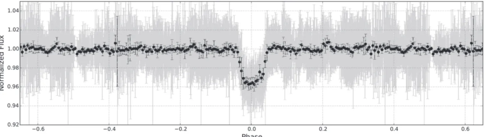
For our study we combined both data sets giving us a light curve with over 6800 data points (TEST:∼6000, BEST:∼800). For the phase folded light curve we measure a standard deviation below 2 mmag in the out-of-transit region using values binned by up 10 minutes. The whole phase folded light curve is shown in Figure1.
2.2. Spectroscopic Observations
Spectroscopic follow-up observations were performed with the Tautenburg 2 m telescope using the Coudé-Echelle spectrograph with an entrance slit that projected to 2″ on the sky. The observed wavelength range covered 4700 and 7400Å with a resolving power(λ/Δλ)of 32,000. For the wavelength Table 1
Technical Parameters of the BEST and TEST Surveys
BEST Survey TEST Survey
Site TLS(2001–2003) TLS
OHP(2005–2006)
Aperture 200 mm 300 mm
Camera AP 10 AP16E
Focal ratio f/2.7 f/3.2
Pixel scale 5.5 arcsec pixel−1 1.9 arcsec pixel−1 Field of view 3°. 1×3°. 1 2°. 2×2°. 2
Readout Time ∼90 s ∼30 s
Exposure Time 240 s 120 s
No. of frames on target 800 6000
Table 2
List of the Photometric Observations of the Eclipsing Binary
BEST TEST
Year Nights Observing Year Nights Observing
[#] (hr) [#] (hr)
2001 3 3.8 2008 7 18.7
2002 10 18.6 2009 31 95.9
2005 4 10.0 2010 3 6.3
2006 6 11.0 2011 34 88.1
calibration, spectra of a Thorium–Argon lamp were taken directly before and after the observations. Stellar spectra were taken with exposure times of 1800 s which resulted in a typical signal-to-noise ratio (S/N)of 20–35. In 2010 a few spectra of the binary system were taken between January and September to get an initial characterization of the transiting system. In 2012 November/December additional spectra were obtained primarily for RV measurements needed to constrain the orbital motion. For the data reduction, standard tools from IRAF were used including bias subtraction, flat-field correction, and wavelength calibration. The RV was determined using the IRAFrvmodule.
3. SYSTEM PARAMETERS
The catalog information of the system is given in Table3.
3.1. Modeling of the Photometric and Radial Velocity Data
A simultaneous fit of the RV and photometric data was performed. The out-of-eclipse part of the light curve did not show any sign of ellipsoidal variation at the level of precision of our observations(Figure1). Therefore we decided to use the spherical model of Mandel & Agol(2002)for the light curve modeling. The expected signal of the secondary transit would have an amplitude of ∼0.1 mmag which would be undetected given our red noise error of 2 mmag. To optimize the fit, we used a genetic algorithm (Geem et al. 2001) to search for the best match between the observed and the modeled light curve. One thousand individuals were used in the population and 300 generations were produced. The bestfit found by this procedure was further refined using a simulated annealing chain(Kallrath & Milone 2009). The error was estimated using 104 random models with values within c2+1s of our best solution. Figure 2 shows 1σ error bars (for details of the code and implementation of the algorithms see Csizmadia et al. 2011). For the light curve modeling we used the unbinned data. The effect of the exposure time was taken into account by using a 4-point Simpson-integration (e.g., Kipping2010).
Free parameters were the scaled semimajor axis ratio a/Rs,
the inclination i, the radius ratio of the two stars R2/R1, the
epoch, the period, theγ-velocity, the semi amplitude of the RV
K, the eccentricity e, the argument of periastron ω, and the combinationu+=ua+ub, whereuaandubare the linear and
the quadratic limb darkening coefficients of the quadratic limb darkening law. The parameteru-=ua -ub was fixed at the
value found by interpolation of the R-band values of Claret & Bloemen (2011). When we performed a fit using free limb darkening combinations as a check, we got
u−=+0.08±0.17, compatible with the previous theoretical value. The other parameters were also within the error bars. The results of thefit are presented in Table4. Figure2shows the phase-folded light curve over-plotted by thefit along with the residuals. Although the noise in single photometric measurements is large, the combined data allow us to reach a Figure 1.The phase-folded light curve. Black points denote data binned to 10 minutes in phase, while the gray points show the original data. Vertical lines show the uncertainties for single measurements.
Table 3
Catalog Information of the Eclipsing Binary Investigated here
Parameter Value
Position 02 40 51. 5h m s +52 45 07d m s
UCAC4 IDa UCAC4 714–021661
2MASS IDb 02405152+5245066
Bmag(UCAC4) 12.287±0.02
Vmag(UCAC4) 11.769±0.02
Jmag(2MASS) 10.771±0.028
Hmag(2MASS) 10.618±0.032
Kmag(2MASS) 10.564±0.026
pmRA(UCAC4) −1.7±0.8 mas yr−1 pmDE(UCAC4) −5.6±1.0 mas yr−1
Notes.Vmag as Given in UCAC4 Catalog(Zacharias et al.2013). a
Zacharias et al.(2013). b
Skrutskie et al.(2006).
precision of ∼2 mmag in 10 minutes bins in the phase folded light curve. The RV data with the bestfit are shown in Figure3.
3.2. Stellar Parameters
To determine the atmospheric parameters of the primary component we created a high quality spectrum by adding all the single observations after applying an RV shift to account for the orbital motion. This resulted in a co-added spectrum with S/N over 90. The analysis was performed over the wavelength range 4740–6400Å. Using the GSSP program
(Grid search in Stellar Parameters; Lehmann et al. 2011; Tkachenko et al.2012).
The normalization of the observed spectra during the reduction is difficult and the results strongly depend on the accuracy of the derived local continuum. We used the comparison of the co-added spectrum with the synthetic ones for an additional continuum correction. The analysis was done in three ways:(a)without any correction,(b)by multiplying the observed spectrum by a factor calculated from a least squares
fit between observed and synthetic spectrum, and c)with a re-normalization applied on smaller scales to get a betterfit to the wings of the Balmer lines (mainly Hβ) and with regions excluded for which the analysis showed distinct deviations of the continuum from the calculated continua. Most of the atmospheric parameters obtained with the three different approaches agreed to within 1σ. However, approach (c)gave a significantly higher value of the effective temperature,
Teff=7350±80 K, which differed by almost 2σ from the
results of the other two methods. This demonstrates the sensitivity ofTeffcaused by small changes in theHβwings.
The parametersTeff, logg,vturb,[Fe/H], andvsin(i)and their
errors were derived using a grid. Thus, the errors include all interdependencies between the parameters. All other metal abundances and their errors were determined separately,fixing all atmospheric parameters to their best fitting values. The formal 1σ error on Teff (80 K) based on error statistics is
probably too small due to systematic errors stemming from the continuum normalization. We use a larger error that includes the systematic error introduced by this normalization.
As determining the stellar parameters is crucial and a possible source of systematic errors in the characterization of the companion, the results have been verified using another method described in Fridlund et al.(2010). Stellar parameters of both methods are in agreement with each other. Only forTeff
we found a larger uncertainty of±200 K. This error agrees with our previousfinding that the normalization of the spectrum can result in an underestimate in the error of the effective temperature and thus the spectral classification. In Table 5
the results for the different approaches are given. For the estimates of mass and radius of the primary star we used the results from the GSSP approach with the small-scale re-normalization(c). For the error estimate ofTeffwe used 250 K
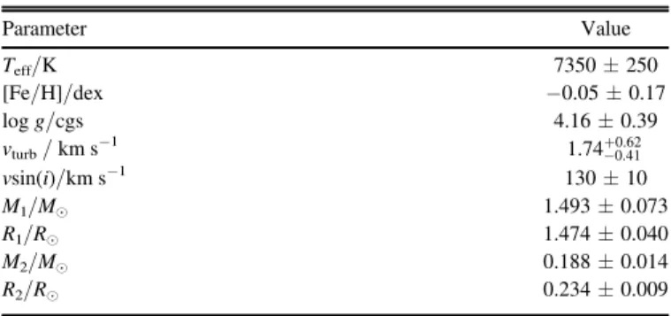
which corresponds to∼3σuncertainty in approach(c). For the primary star we found an effective temperature
Teff=(7350 K±250)K, asurface gravity of logg=(4.16±
0.39)cgs, and a metalicity of[Fe/H]=(−0.05±0.17)dex. The mass of the primary star M1 was derived using
PARSEC1.2S isochrones (Bressan et al. 2012; Chen et al.2014, 2015; Tang et al. 2014) in combination with the stellar parameters and 2MASS color information (Cutri et al.
2003). The radius of the primary is given by its mass and surface gravity. From the mass function f(m) we derived the mass of the secondary object as M2=(0.188±0.014)Me. The radius of the secondary was calculated using the radius of the primary and the ratioR2/R1that comes from the light curve
modeling R2=(0.234±0.009)Re. The resulting system
mass (M1+M2), radius of the primary (R1), semimajor axis a/R1, and orbital period were tested for satisfying Kepler’s
third law.
We compared our results using the PARSEC1.2S model with those using the Y2 stellar models (Yi et al. 2001; Demarque et al.2004)and the Dartmouth model(Dotter et al.
2008). All three models are in agreement and give us the similar results(within 1σ)for the mass and radius of the binary components. The Dartmouth model results in binary compo-nents that are a bit smaller and less massive, whereas the Y2 model suggests larger and more massive stars.
The atmospheric and bulk parameters of both stars are listed in Table6.
Table 4
Modeling Parameters
Parameter Value
a/R1 4.12±0.06
b 0.45±0.03
i 84°. 1±0°. 3
R2/R1 0.1601±0.0017
u+ 1.05±0.07
u− −0.02(fixed)
e 0.070±0.063
ω 227°±13°
P 1.35121 days±1×10⁻⁵days
Epoch 2452196.1196±0.0032 HJD
γ-velocity (30.50±0.50)km s−1
K (26.10±0.76)km s−1
Note.The given errors correspond to the 1σuncertainties.a/R1; the impact parameterb(bwas calculated viab a e 1 sin i sin v
e v 1 1 cos
2 2
0 2
0 ·
·( ) ·
= - *
-+ where
v0=90 -w+qthe mean anomaly at the mid-transit moment, see Gimenez & Garcia-Pelayo(1983)); the inclinationiof the system; the radius ratioR2/R1; the limb darkening coefficientsu+andu−; the eccentricityeof the system; the periodP; the epoch of the system and the radial velocity semi amplitudeK.
3.3. Synchronization of the System
In order to assess whether the system is synchronized we computed the synchronization factor comparing the rotational period of the star with the orbital period. If a 1:1 spin–orbit synchronization and alignment has taken place the rotation period of the primary star is equal to the orbital period of the system. We assume the orbital inclination to be nearly the same as the rotational inclination. The rotational velocity of the primary star derived from the spectral line broadening is
vsini=(130±10)km s−1. We know the inclination of the orbital plane to be i=84°. 1±0°. 3 from the light curve modeling. With the radius of the primary star and its real rotational velocityV v i
i
rot sin sin
= we derive the rotational period
Prot=2* p*R V1 rot=(0.580.06 days) . This gives the synchronization factor of Prot/Porb=0.43±0.05.
The system is clearly not in a 1:1 synchronization, but the rotational period of the primary star and the orbital period are close to a 2:1 commensurability. Even if the orbital inclination would not be the same as the rotational inclination our conclusion would still stand as the synchronization factor would only decrease for smaller inclinations.
Normally, we expect close binary stars to evolve into a 1:1 spin–orbit resonance if the eccentricity is close to 0. As shown by Celletti et al. (2007), Celletti & Chierchia (2008) for examples of the solar system the 2:1 resonances are very unlikely for objects in low eccentricity orbits. Our light curve and RV modeling suggest an eccentricity close to 0. This makes it unlikely for the system to be in a dynamically stable 2:1 resonance. The observed commensurability is likely not to
be a stable resonance, but a mere coincidence. As shown in the analysis by Béky et al. (2014), the assumption that every commensurability is due to stable dynamical resonances is implausible.
If the binary is not yet synchronized this can only mean that it is younger than the time scale of synchronization. This time scale for the system,átsyncñ, was computed according to Zahn
(1977)and Hilditch(2001). Using the stellar models grids by Claret(2004), we determined the radius of gyrotation and the tidal torque constant of the primary star. For this system the time scale of synchronization lies in the range between 120 and 250 Myr. If no third body is preventing the system from synchronization, this system looks younger than 250 Myr.
For the age of the primary star we get no conclusive result, but Parsec1.2S isochrones suggest ages below 1.4 Gyr. In Figure4the mass and radius of the primary star is plotted along with various isochrones.
4. DISCUSSION
The mass–radius relations given by the stellar evolution models of Baraffe et al. (1998) and Bressan et al. (2012), Table 5
Results of Stellar Analysis with the GSSP Program and the Method describe in Fridlund et al.(2010)
Parameter GSSP Method 2
Parameter (a) (b) (c)
Teff/K 7150±80 7130±80 7350±80 7300±200
[Fe/H]/dex −0.02±0.15 −0.2±0.2 −0.15±0.17 0.0±0.2
logg/cgs 3.98±0.38 3.96±0.34 4.16±0.39 4.1±0.3
vsin(i)/km s−1 127±9 126±10 130±10 125±10
Note.For the former analysis three different normalizations of the spectrum were tested:(a)without any correction,(b)by multiplying the observed spectrum by a factor calculated from a least squaresfit between observed and synthetic spectrum, and(c)with a re-normalization applied on smaller scales.
Table 6
Bulk Parameters for both Stars
Parameter Value
Teff/K 7350±250
[Fe/H]/dex −0.05±0.17
logg/cgs 4.16±0.39
vturb/km s−1 1.74-+0.410.62
vsin(i)/km s−1 130±10
M1/Me 1.493±0.073
R1/Re 1.474±0.040
M2/Me 0.188±0.014
R2/Re 0.234±0.009
Note.Teff, Fe/H, and logg were determined using a grid search. For the parameters derived from spectral analysis the 1σerror is given. ForTeffa 3σ error is listed. Masses and radii including their errors, were determined using the according isochrones, the results from light curve modeling, and thefitted radial velocity measurements.
indicate that the low mass companion has an inflated radius. The empirical mass–radius relations of Mann et al.(2015)and Boyajian et al. (2012) suggests that stellar evolution models systematically underestimate the stellar radius of very low-mass stars by∼5%. For VLMSs with masses below 0.3Methe data presented in Mann et al.(2015)also shows discrepancy in the mass by∼4% compared to the Dartmouth model. However, Mann et al. (2015)suggest that the model inferred masses are more reliable than the empirically derived ones. It thus is more suited to compare our results with model isochrones that are corrected for the underestimated radius. These corrected isochrones show that the M dwarf is slightly inflated. Such an anomalous radius could be explained by the youth of the star.
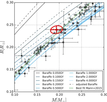
Figure 5 shows our M dwarf in relation to other known systems with masses and radii below 0.3Me and 0.3Re, respectively. Crosses represent eclipsing binaries and single stars studied with interferometry. Circles represent spectro-scopically characterized VLMSs. The lines show isochrones by Baraffe et al.(1998)with metallicity[M/H]=0.0 of different ages. The dashed lines show the isochrones corrected for a radius underestimated by 5%. The green dashed line shows a polynomialfit of third order to the mass–radius relation for the data presented in Mann et al. (2015). Discrepancies between the empirical data from Mann et al. (2015) and the adjusted isochrones are due to the underestimate in masses for VLMSs. The empirical mass–radius relation for low-mass stars is based on objects typically of several Gyr in age. Due to the limited
number of young VLMSs it is not clear whether stellar models also underestimate the radius by 5% for young stars. Never-theless, taking into account the underestimate in the radius by the stellar models as it is known for older stars, the mass–radius relation of the M dwarf agrees best with the isochrones for ages between 100 and 200 Myr.
Comparison of the stellar parameters for the primary star with isochrones do not allow us to constrain further the age of the system, but our results hint toward a young system. Isochrones from different stellar models all suggest an age below 1 Gyr. Furthermore, the system is not in a 1:1 spin–orbit resonance, which we would expect for such binary system with an eccentricity close to 0.
The stellar rotation of the primary star is close to a 2:1 commensurability with the orbital period. Similar commensur-abilities were found in some exoplanetary systems (see Béky et al. 2014) and in the brown dwarf system CoRoT-33
(Csizmadia et al. 2015), but have not yet been reported for binary systems.
It is unlikely that these 2:1 resonant systems of low eccentricities are dynamically stable (Celletti & Chierchia 2008). As pointed out in the study by Béky et al.
(2014)there are good reasons to believe that such commensur-abilities are a statistical phenomena and not a stable resonance. We see two possibilities why this system is not tidally locked. Either the system is younger than the time scale of synchronization, which is below 250 Myr, or a third body is present that perturbs the system. However, wefind no evidence for this third body in the photometric or RV data. Long-term high precision RV monitoring, or AO imaging of this star may reveal a third body. At the present time, all the available evidence from the dynamical analysis of of the system combined with the mass–radius relationship of both compo-nents point to a system that is younger than 250 Myr.
In contrast to M dwarfs older than 500 Myr, where the differences between stellar evolution models are small compared to observational errors, isochrones of ages below 250 Myr differ significantly between models. Given the uncertainties in the stellar parameters it is not yet possible to distinguish between different stellar models for this M dwarf. But with the expected age of the system below the time scale of synchronization, which is in agreement with the mass–radius relation of the low mass companion, this system is a unique test object for stellar evolution models. It is one of the youngest studied M dwarfs in an eclipsing binary. Better values of the stellar parameters, particularly the stellar age of the primary star, will allow to test different stellar evolution models. Additionally this system can serve as an interesting test object for rotational evolution of low-mass stars in presence of a close companion and possibly strong stellar wind(c.f. Ferraz-Mello et al.2015).
5. CONCLUSION
We characterized a DEB system with un-equal mass components comprised of a very low-mass M dwarf orbiting an early F-type main-sequence star. The system was investi-gated combining photometric data and RV measurements. Using stellar evolution models we determined the bulk properties of the primary star. Using different stellar models for the characterization of the primary star did not lead to significant changes in the mass–radius relation of either of the stars.
Figure 5. Mass radius relation of very low-mass stars. Plotted are stars in eclipsing binaries(gray circles) (Ségransan et al.2003; Bouchy et al.2005; Pont et al.2005,2006; Hebb et al.2006; Beatty et al.2007; Maxted et al.2007; Blake et al.2008; Fernandez et al.2009; Morales et al.2009; Vida et al.2009; Dimitrov & Kjurkchieva2010; Parsons et al.2010,2012; Hartman et al.2011; Carter et al.2011; Irwin et al.2011; Pyrzas et al.2012; Nefs et al.2013; Tal-Or et al. 2013; Gómez Maqueo Chew et al. 2014; Zhou et al. 2014) and spectroscopic characterized single low mass stars(gray triangles) (Mann et al.
The orbital period is 1.35121±0.00001 days. The mass of the M dwarf is M2=0.188±0.014Me. With a radius of
R2=0.234±0.009Rethe M dwarf is slightly inflated even
when taking into account that current stellar models under-estimate the radii of low-mass stars by∼5%.
The low density of the M dwarf star could be explained by an age of the system between 100 and 250 Myr. The spectral characterization of the primary star does not allow us to further constrain the age of the system. However, the system has not yet reached the 1:1 spin–orbit resonance, which we would expect for such a close binary with a nearly circular orbit. This supports the conclusion that the age of the system is below 250 Myr.
The M dwarf thus is one of the youngest characterized main-sequence M dwarfs in an eclipsing binary system. Additionally, it is one of the very few VLMSs which allows us to estimate the age estimate without isochrone fitting. It might play a crucial role in further understanding of the mass–radius relation for young very low mass objects. The system is also of high interest with regard to the dynamical interactions in such close binaries.
Part of this work was supported by the Deutsche Forschungsgemeinschaft DFG under projects Ei409/14-1,-2. SzCs acknowledges the support under the Hungarian OTKA Grant K113117. IRAF is distributed by the National Optical Astronomy Observatory, which is operated by the Association of Universities for Research in Astronomy (AURA) under cooperative agreement with the National Science Foundation. PyRAF and PyFITS were used for this work and are products of the Space Telescope Science Institute, which is operated by AURA for NASA. This work is based in part on observations obtained with the 2 m Alfred Jensch Telescope of the Thüringer Landessternwarte Tautenburg. We thank the referee for the detailed comments which have improved this paper.
Facility: TLS(2 m Coude, TEST).
REFERENCES
Aerts, C., Christensen-Dalsgaard, J., & Kurtz, D. W. 2010, Asteroseismology
(Berlin: Springer)
Andersen, J. 1991,A&ARv,3, 91
Baraffe, I., Chabrier, G., Allard, F., & Hauschildt, P. H. 1998, A&A,337, 403
Barnes, S. A. 2010,ApJ,722, 222
Beatty, T. G., Fernández, J. M., Latham, D. W., et al. 2007,ApJ,663, 573
Béky, B., Holman, M. J., Kipping, D. M., & Noyes, R. W. 2014,ApJ,788, 1
Berger, D. H., Gies, D. R., McAlister, H. A., et al. 2006,ApJ,644, 475
Blake, C. H., Torres, G., Bloom, J. S., & Gaudi, B. S. 2008,ApJ,684, 635
Bouchy, F., Pont, F., Melo, C., et al. 2005,A&A,431, 1105
Boyajian, T., von Braun, K., Feiden, G. A., et al. 2015,MNRAS,447, 846
Boyajian, T. S., von Braun, K., van Belle, G., et al. 2012,ApJ,757, 112
Bressan, A., Marigo, P., Girardi, L., et al. 2012,MNRAS,427, 127
Carter, J. A., Fabrycky, D. C., Ragozzine, D., et al. 2011,Sci,331, 562
Celletti, A., & Chierchia, L. 2008,CeMDA,101, 159
Celletti, A., Froeschlé, C., & Lega, E. 2007,P&SS,55, 889
Chen, Y., Bressan, A., Girardi, L., et al. 2015,MNRAS,452, 1068
Chen, Y., Girardi, L., Bressan, A., et al. 2014,MNRAS,444, 2525
Claret, A. 2004,A&A,424, 919
Claret, A., & Bloemen, S. 2011,A&A,529, A75
Clausen, J. V., Frandsen, S., Bruntt, H., et al. 2010,A&A,516, A42
Csizmadia, Sz., Hatzes, A., Gandolfi, D., et al. 2015,A&A,584, A13
Csizmadia, Sz., Moutou, C., Deleuil, M., et al. 2011,A&A,531, A41
Cutri, R. M., Skrutskie, M. F., van Dyk, S., et al. 2003, 2MASS All Sky Catalog of Point Sources,http://irsa.ipac.caltech.edu/applications/Gator
David, T. J., Hillenbrand, L. A., Cody, A. M., Carpenter, J. M., & Howard, A. W. 2016,ApJ,816, 21
Delorme, P., Collier Cameron, A., Hebb, L., et al. 2011,MNRAS,413, 2218
Demarque, P., Woo, J.-H., Kim, Y.-C., & Yi, S. K. 2004,ApJS,155, 667
Demory, B.-O., Ségransan, D., Forveille, T., et al. 2009,A&A,505, 205
Dimitrov, D. P., & Kjurkchieva, D. P. 2010,MNRAS,406, 2559
Dotter, A., Chaboyer, B., Jevremović, D., et al. 2008,ApJS,178, 89
Drake, S. A., Pravdo, S. H., Angelini, L., & Stern, R. A. 1998,AJ,115, 2122
Eigmüller, P. 2012, PhD thesis, Friedrich-Schiller-Universität Jena
Eigmüller, P., & Eislöffel, J. 2009, in IAU Symp. 253, Transiting Planets, ed. F. Pont, D. Sasselov, & M. J. Holman, 340
Fernandez, J. M., Latham, D. W., Torres, G., et al. 2009,ApJ,701, 764
Ferraz-Mello, S., Tadeu dos Santos, M., Folonier, H., et al. 2015,ApJ,807, 78
Fridlund, M., Hébrard, G., Alonso, R., et al. 2010,A&A,512, A14
Fruth, T., Cabrera, J., Chini, R., et al. 2013,AJ,146, 136
Fruth, T., Kabath, P., Cabrera, J., et al. 2012,AJ,143, 140
Geem, Z. W., Kim, J. H., & Loganathan, G. 2001,Simul, 76, 60 Gimenez, A., & Garcia-Pelayo, J. M. 1983,Ap&SS,92, 203
Gómez Maqueo Chew, Y., Morales, J. C., Faedi, F., et al. 2014, A&A,
572, A50
Hartman, J. D., Bakos, G. Á., Noyes, R. W., et al. 2011,AJ,141, 166
Hebb, L., Wyse, R. F. G., Gilmore, G., & Holtzman, J. 2006,AJ,131, 555
Hilditch, R. W. 2001, An Introduction to Close Binary Stars (Cambridge: Cambridge Univ. Press)
Irwin, J. M., Quinn, S. N., Berta, Z. K., et al. 2011,ApJ,742, 123
Kallrath, J., & Milone, E. F. 2009, Eclipsing Binary Stars: Modeling and Analysis(New York: Springer-Verlag)
Kipping, D. M. 2010,MNRAS,408, 1758
Klagyivik, P., Csizmadia, Sz., Pasternacki, T., et al. 2013,ApJ,773, 54
Kraus, A. L., Cody, A. M., Covey, K. R., et al. 2015,ApJ,807, 3
Lane, B. F., Boden, A. F., & Kulkarni, S. R. 2001,ApJL,551, L81
Lebreton, Y., Goupil, M. J., & Montalbán, J. 2014a, in EAS Publications Series 65, How Accurate are Stellar Ages Based on Stellar Models? I. The Impact of Stellar Models(Les Ulis, France: EDP Sciences), 99
Lebreton, Y., Goupil, M. J., & Montalbán, J. 2014b, in EAS Publications Series 65, How Accurate are Stellar Ages Based on Stellar Models? II. The Impact of Asteroseismology(Les Ulis, France: EDP Sciences), 177 Lehmann, H., Tkachenko, A., Semaan, T., et al. 2011,A&A,526, A124
López-Morales, M. 2007,ApJ,660, 732
Mandel, K., & Agol, E. 2002,ApJL,580, L171
Mann, A. W., Feiden, G. A., Gaidos, E., Boyajian, T., & von Braun, K. 2015,
ApJ,804, 64
Maxted, P. F. L., O’Donoghue, D., Morales-Rueda, L., Napiwotzki, R., & Smalley, B. 2007,MNRAS,376, 919
Morales, J. C., Ribas, I., Jordi, C., et al. 2009,ApJ,691, 1400
Nefs, S. V., Birkby, J. L., Snellen, I. A. G., et al. 2013,MNRAS,431, 3240
Parsons, S. G., Gänsicke, B. T., Marsh, T. R., et al. 2012,MNRAS,426, 1950
Parsons, S. G., Marsh, T. R., Copperwheat, C. M., et al. 2010, MNRAS,
402, 2591
Pasternacki, T., Csizmadia, Sz., Cabrera, J., et al. 2011,AJ,142, 114
Pont, F., Melo, C. H. F., Bouchy, F., et al. 2005,A&A,433, L21
Pont, F., Moutou, C., Bouchy, F., et al. 2006,A&A,447, 1035
Pyrzas, S., Gänsicke, B. T., Brady, S., et al. 2012,MNRAS,419, 817
Rauer, H., Eislöffel, J., Erikson, A., et al. 2004,PASP,116, 38
Ribas, I. 2006,Ap&SS,304, 89
Ségransan, D., Kervella, P., Forveille, T., & Queloz, D. 2003,A&A,397, L5
Skrutskie, M. F., Cutri, R. M., Stiening, R., et al. 2006,AJ,131, 1163
Spada, F., Demarque, P., Kim, Y.-C., & Sills, A. 2013,ApJ,776, 87
Tal-Or, L., Mazeh, T., Alonso, R., et al. 2013,A&A,553, A30
Tamuz, O., Mazeh, T., & Zucker, S. 2005,MNRAS,356, 1466
Tang, J., Bressan, A., Rosenfield, P., et al. 2014,MNRAS,445, 4287
Tkachenko, A., Lehmann, H., Smalley, B., Debosscher, J., & Aerts, C. 2012,
MNRAS,422, 2960
Torres, G. 2013, AN,334, 4
Torres, G., Andersen, J., & Giménez, A. 2010,A&ARv,18, 67
van Belle, G. T., & von Braun, K. 2009,ApJ,694, 1085
Vida, K., Oláh, K., Kővári, Z., et al. 2009,A&A,504, 1021
Voss, H. 2006, PhD thesis, Technische Universität Berlin Yi, S., Demarque, P., Kim, Y.-C., et al. 2001,ApJS,136, 417
Zacharias, N., Finch, C. T., Girard, T. M., et al. 2013,AJ,145, 44
Zahn, J.-P. 1977, A&A,57, 383