McBride_unc_0153D_16019.pdf

(1)

STAR FORMATION HISTORIES OF SOUTHERN COMPACT GROUPS

JoEllen McBride

A dissertation submitted to the faculty at the University of North Carolina at Chapel Hill in partial fulfillment of the requirements for the degree of Doctor of Philosophy in the Department of Physics.

Chapel Hill 2016

Approved by:

Gerald Cecil

Chris Clemens

Fabian Heitsch

Christian Iliades

(2)

(3)

ABSTRACT

JoEllen McBride: Star Formation Histories of Southern Compact Groups (Under the direction of Gerald Cecil)

(4)

ACKNOWLEDGEMENTS

(5)

TABLE OF CONTENTS

LIST OF TABLES . . . vii

LIST OF FIGURES . . . viii

LIST OF ABBREVIATIONS AND SYMBOLS . . . ix

1: Introduction . . . 1

1.1 Motivation . . . 1

1.2 Compact Groups . . . 4

1.2.1 Hickson Compact Groups . . . 5

1.2.2 Recent Compact Group Surveys . . . 8

1.2.3 Southern Compact Groups . . . 9

1.3 Multi-object Spectroscopy . . . 11

1.4 Integral Field Spectroscopy . . . 11

1.5 Dissertation Outline . . . 14

2: Dissertation Design . . . 15

2.1 Science Questions . . . 15

2.2 Extra-galactic Stellar Populations . . . 16

2.2.1 History of Stellar Population Analysis . . . 16

2.2.2 Compact Group Stellar Populations . . . 20

2.2.3 STARLIGHT . . . 21

2.3 Emission Line Fitting . . . 29

2.3.1 History of Emission Line Measurements . . . 29

2.3.2 Compact Group Emission Line Results . . . 32

(6)

2.4 CINDERS Experiment Design . . . 33

2.4.1 Observing set-up . . . 33

2.4.2 Sensitivity Analysis/Simulations . . . 34

2.4.3 Target Selection . . . 39

2.5 MOS Procedure . . . 43

3: Instrumentation Results . . . 45

3.1 CINDERS . . . 45

3.1.1 CINDERS Design . . . 45

3.1.2 CINDERS Construction . . . 48

3.1.3 CINDERS Commissioning . . . 52

3.1.4 CINDERS Status . . . 55

3.2 MOS . . . 55

3.2.1 MOS Design and Construction . . . 55

3.2.2 MOS Commissioning and Status . . . 56

4: Data and Results . . . 58

4.1 Data . . . 58

4.2 Reduction and Processing . . . 60

4.3 Analysis . . . 63

4.3.1 Examples of Spectra . . . 68

4.3.2 SCG08 . . . 78

4.3.3 SCG13 . . . 89

4.3.4 SCG68 . . . 102

4.3.5 SCG72 . . . 114

(7)

4.3.9 SCG106 . . . 161

4.3.10 SCG62 . . . 172

4.3.11 SCG07 . . . 184

4.3.12 All Galaxies . . . 195

5: Summary and Future Work . . . 201

A: STARLIGHT Analysis Results. . . 208

A.1 Age and Z Single Population Bracket Analysis . . . 208

A.1.1 Young Age Bracket Analysis . . . 208

A.1.2 Intermediate Age Bracket Analysis . . . 209

A.1.3 Old Age Bracket Analysis . . . 209

A.1.4 Low Z Bracket Analysis . . . 209

A.1.5 Mid Z Bracket Analysis . . . 210

A.1.6 High Z Bracket Analysis . . . 210

A.2 Single and Mixed Population Analysis . . . 211

A.2.1 Single Population All Age and Z Residuals . . . 211

A.2.2 Two Population All Age and Z Residuals . . . 212

A.2.3 Three Population All Age and Z Residuals . . . 213

A.3 Number of Base Templates Analysis . . . 214

A.3.1 Age Residuals . . . 214

A.3.2 Z Residuals . . . 215

B: CINDERS Observations . . . 217

(8)

LIST OF TABLES

1.1 Prior IFU Survey Properties . . . 12

1.2 Current and Future IFS systems . . . 13

2.1 Templates used for analysis. . . 26

2.2 Total templates fit and not fit by intermediate populations. . . 27

2.3 Fraction of light due to young, intermediate and old template components. . . 28

2.4 Emission lines potentially present in my spectra. . . 33

2.5 Observation set-up . . . 34

2.6 Atmospheric Extinction over Mauna Kea . . . 37

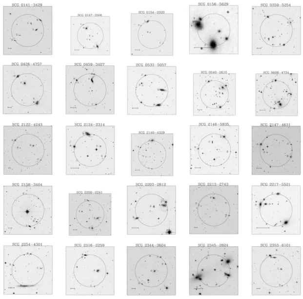
2.7 Images of SCGs where all group members are observable. . . 40

4.1 SCG observations. Observations with ∗ were not used in this analysis. . . 59

4.2 Table of spectrophotometric standard observations. . . 60

4.3 Derived redshift differences for group SCG08. . . 78

4.4 Stellar population and activity analysis summary for SCG08. I abbreviate the age and metallicity designations as young (Y), intermediate (I), old (O), low (L), mid (M) and high (H), and the region designations as central (c), middle (m), and all (a). . . 89

4.6 Stellar population and activity analysis summary for SCG13. Same codes as in Table 4.4 . . . . 102

(9)

4.23 Interaction code for each galaxy. . . 200

A.1 Age residuals for young age brackets. Values are in dex. . . 208

A.2 Age residuals for intermediate age brackets. Values are in dex. . . 209

A.3 Age residuals for old age bracket. Values are in Gyrs. . . 209

A.4 Z residuals for low Z brackets. Values are in [M/H]. . . 209

A.5 Z residuals for mid Z brackets. Values are in [M/H]. . . 210

A.6 Z residuals for high Z bracket. Values are in [M/H]. . . 210

A.7 Residuals for single populations. Ages are reported asLog(t), Z is in [M/H]. . . 211

A.8 Residuals for two populations. Ages are reported asLog(t), Z is in [M/H]. . . 212

A.9 Residuals for three populations. Ages are reported asLog(t), Z is in [M/H]. . . 213

A.10 Residuals for all young populations. Ages are reported asLog(t). . . 214

A.11 Residuals for all intermediate populations. Ages are reported asLog(t). . . 214

A.12 Residuals for all old populations. Ages are reported asLog(t). . . 215

A.13 Residuals for all low Z populations. Zs are in [M/H]. . . 215

A.14 Residuals for all mid Z populations. Zs are in [M/H]. . . 216

A.15 Residuals for all high Z populations. Zs are in [M/H]. . . 216

B.1 First pass of observations . . . 217

B.2 Second pass of observations . . . 218

(10)

LIST OF FIGURES

1.1 The relationship between surface mass density (µ∗) (left) and concentration index (C=R90/R50) (right) and stellar mass for galaxies in density bins of 0-1 neighbor (cyan), 2-3 neighbors (green), 4-6 neighbors (blue), 7-11 neighbors (black), 12-16 neighbors (red), >17 neighbors (magenta). Neighbors are defined within a 2 Mpc projected radius and±500 km/s velocity difference of a target galaxy. The solid curves are the median values of surface mass density and concentration index for each mass bin and the dotted lines denote the 10th and 90th percentiles.[8] . . . 2 1.2 The relationship between the median values of Dn(4000) (top left) and SF R/M∗ (top right)

and stellar mass for galaxies in previously defined density bins. Plots of the median value of

Dn(4000) and surface mass density (bottom left) and concentration index (bottom right) are also shown. [8] . . . 2 1.3 Relation between star formation history propertiesSF R/M∗,Dn(4000) andHδA. Solid circles

are the median values, open and solid triangles are the 25th and 75th percentile and open and solid squares are the 10th and 90th percentiles respectively. [8] . . . 3 1.4 Left plot is of galaxies containing strong AGN with respect to stellar mass in three different

density bins; 0-1 neighbor (cyan), 7-11 neighbors (black) and >12 neighbors (red). The right plot shows the distribution of [OIII] luminous AGNs in low and high density environments. [8] . 3

2.1 Color versus age for three types of metallicity[106]. Higher V −I values correspond to redder colors. . . 16 2.2 Theoretical HR diagrams from [107]. Tracks follow how the luminosity and temperature of a

star at a given mass changes throughout its lifetime. The plot on the left is for low mass stars and the plot on the right is for intermediate mass and massive stars. Stars in both plots have compositionY = 0.230 andZ= 0.0001. The mass of each star is indicated in solar masses next to each curve. . . 17 2.3 Isochrones derived from theoretical HR diagrams by [107]. Ages span fromlog(age/yr) = 6.8−

10.2 in intervals of 0.2. . . 18 2.4 Table 1 from [123] which lists the properties of the most commonly used stellar templates. . . . 20 2.5 MILES metallicity properties plotted over the Padova isochrones. MILES covers the lower main

sequence and RGB phases at both metallicities.[139] . . . 22 2.6 Examples of MILES template spectra with normalized flux. The plot on the left shows spectra for

different ages with solar metallicity. The plot on the right shows spectra for different metallicities at 1.0 Gyrs. Spectra are offset by a constant flux so spectral features can be seen. . . 22 2.7 Age vs Lick indice for 294 MILES templates. . . 23 2.8 Age vs Lick indice plots showing young (blue squares), intermediate (green x) and old (red circle)

(11)

2.11 Diagnostic Lines . . . 34

2.12 Color vs Age for SSPs with different metallicities. . . 35

2.13 SOAR throughput. . . 37

2.14 Environmental parameters. . . 41

2.15 Group luminosity and color parameters. . . 42

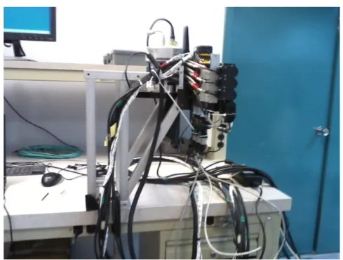
3.1 CINDERS positioning on the Goodman apparatus. 1) shows the CINDERS probes placed in front of the slit mask assembly. The region to the right off the image is where the light input from the primary telescope mirror is fed. 2) shows ourf /5 collimator attached to the end of the current Goodman collimator. The protruding cylinder is where the output ends of the bundles are placed. Our collimator is fed through the grating, blue filter wheel and on into the camera, which is located to the left of the image. . . 46

3.2 Left image: SolidWorks rendering of the x, y and z motion apparatus. The ANDOR camera and its field mirror are shown behind the rail positioner. Right image: Zoomed in on the z motion probe. . . 47

3.3 SolidWorks rendering of the slit block attached to the collimator. . . 48

3.4 Left image: Front view of CINDERS. Right image: Front view of probes with prisms and lenses installed. . . 49

3.5 Side view of CINDERS to show ANDOR camera and field mirror. . . 49

3.6 Left image: Slit block assemble that attaches to collimator. Right image: Showing glass block alignment. . . 50

3.7 Left image: Top end of silk sheath with bundles. Right image: Sheath and bundles inside incompressible tube. . . 50

3.8 Left image: Glass block ends of fibers epoxied to increase strength and help prevent break-age. Right image: Bundle support for routing bundle and incompressible tube over gantry and collimator. . . 51

3.9 Left image: Image of probe control GUI. Right image: Output of CINDERS Field Viewer. . . . 52

3.10 Solid Works rendering of attachment to reliably hold probe onto y-motion assembly. . . 53

3.11 Probe entrance indicated on back of circuit board with white out. . . 54

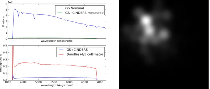
3.12 Left image: Throughtput for Bundle 3 on standard star HR3454. Right image: Reconstructed image of Bundle 3. . . 55

3.13 Screenshot of MOS Slit Designer tool. . . 56

(12)

4.1 The top two plots are of theχ2values for our fits as a function of S/N in the blue and red regions of the observed spectrum. The bottom two plots show the percent deviation of the fitted model

|Oλ−Mλ|

Mλ as a function of S/N. The percent deviations are level starting at around a S/N of 15. . 64

4.2 Flowchart for determining SP properties. . . 65

4.3 Emission spectrum and fit for SCG08 Galaxy A. The black line is the observation and the red line is the fit. The bottom plot shows the residuals of the fit, note vertical scale change. . . 66

4.4 Region color coding. . . 67

4.5 Central extractions for SCG88 B. . . 68

4.6 Outer extractions for SCG88 B. . . 69

4.7 Central extractions for SCG68 A. . . 69

4.8 Outer extractions for SCG68 A. . . 70

4.9 Central extractions for SCG08 A. . . 71

4.10 Outer extractions for SCG08 A. . . 72

4.11 Central extractions for SCG13 B. . . 73

4.12 Outer extractions for SCG13 B. . . 74

4.13 Central extractions for SCG08 C. . . 75

4.14 Outer extractions for SCG08 C. . . 76

4.15 Central extractions for SCG62 D. . . 77

4.16 Outer extractions for SCG62 D. . . 77

4.17 Group SCG08. . . 78

4.18 Galaxy distribution for SCG08. . . 79

4.19 Age and metallicity plots for the extracted spectra of galaxies in SCG08. . . 80

4.20 Age and metallicity plots for the 10” bin spectra of galaxies in SCG08. . . 81

(13)

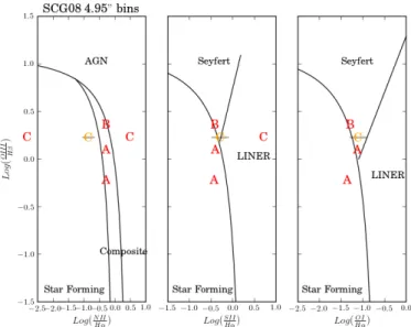
4.27 BPT diagrams for the 3” bin spectra of galaxies in SCG08. . . 86

4.28 BPT diagrams for the 1” bin spectra of galaxies in SCG08. . . 87

4.29 Stellar population results for the 5” and 3” bins and activity information for the 1” bins for SCG08. 88 4.30 Group SCG13. . . 90

4.37 Activity plots for the extracted spectra of galaxies in SCG13. . . 97

4.38 Activity plots for the 10” bin spectra of galaxies in SCG13. . . 97

4.42 Stellar population results for the 5” and 3” bins and activity information for the 1” bins for SCG13.101 4.43 Group SCG68. . . 103

(14)

4.54 Group SCG72. . . 115

(15)

(16)

4.114 Stellar population results for the 5” and 3” bins and activity information for the 1” bins for SCG106. . . 171

4.115 Group SCG62. . . 173

4.116 Group SCG62. . . 174

4.126 Group SCG07. . . 185

4.127 Group SCG07. . . 186

(17)

4.138 Age and metallicity plots for all galaxies in a group. . . 196

4.139 BPT diagrams for all galaxies in a group. . . 197

4.140 SP properties for all SF galaxies in a group. . . 198

4.141 SP properties for all active galaxies other than SF in a group. . . 199

5.1 Summaries for group members. I abbreviate the age and metallicity designations as young (Y), intermediate (I), old (O), low (L), mid (M) and high (H), and the region designations as central (c), middle (m), and all (a). . . 203

5.2 Summaries for group members continued. . . 204

(18)

LIST OF ABBREVIATIONS AND SYMBOLS

2MASS Two Micron All Sky Survey

a All regions

AAT Australia Astronomical Telescope ADC Atmospheric Dispersion Corrector AGN Active Galactic Nuclei

AMIGA Analysis of the interstellar Medium of Isolated GAlaxies APO Apache Point Observatory

BPT Baldwin, Phillips & Terlevich

c Central region

cm Central + Middle region

CALIFAS Calar Alto Legacy Integral Field Area Survey CCD Charged Coupled Device

CIG Catalog of Isolated Galaxies

CINDERS Circularized IFUs Nearly Deployed using Economical Robots on SOAR

DM Disturbed morphology

e Edge region

FITS Flexiable Image Transport System

FLAMES Fibre Large Array Multi Element Spectrograph

FOV Field of View

FWHM Full Width at Half Maximum GAMA Galaxy And Mass Assembly

H High metallicity

HCG Hickson Compact Group

(19)

IDS Image Dissector Scanner IFS Integral Field Spectroscopy IFU Integral Field Unit

IMF Initial Mass Function

L Low metallicity

LLAGN Low Luminosity Active Galactic Nuclei LINERS Low-Ionization Nuclear Emission-line Regions

LR Low Resolution

M Mid metallicity

m Middle region

me Middle+Edge region

MANGA Mapping Nearby Galaxies at APO

MILES Medium resolution Isaac Newton Telescope Library of Empirical Spectra MOS Multi-Object Spectroscopy

NGC Nearby Galaxies Catalog

O Old Age

POSS Palomar Observatory Sky Survey

PPAK Pmas fiber PAcK

PROMPT Panchromatic Robotic Optical Monitoring and Polarimetry Telescopes RSCG Redshift Selected Compact Group

SAM SOAR Adaptive optics Module

SAMI Sydney-AAO Multi-object Integral field

SAURON Spectrographic Areal Unit for Research on Optical Nebulae

SB Starburst

(20)

SF Star Formation

SFH Star Formation History SFR Star Formation Rate S/N Signal-to-Noise

SOAR SOuthern Astrophysical Research SP Stellar Population

SSP Simple Stellar Populations

UKST United Kingdom Schmidt Telescope VENGA VIRUS-P Exploration of Nearby Galaxies VLT Very Large Telescope

Y Young age

” Arcsecond

’ Arcminute

˚

A Angstrom

[_{F e}α] Mass fraction of heavy elements (C...) compared to that of Fe

Bj 3200−5500˚A filter of POSS plates used in Iovino, 2002. C=R90/R50 Concentration index

dm Incremental mass element

∆magcomp Bj magnitude difference between the faintest and brightest group member.

∆magisol Bj magnitude difference between the brightest galaxy in the isolation ring (Risol) and the

brightest group member

∆µgr Difference between the mean surface brightness within the isolation ring (µisol) and the group

(µgr) Dn(4000) 4000˚A break

(21)

Hβ Hydrogenβ line at 486nm rest wavelength

Hγ Hydrogenγline at 434nm rest wavelength

Hδ Hydrogenδline at 410nm rest wavelength

HδA Hydrogenδline equivalent width

j Emission line intensity

LF IR

Lopt Far infrared luminosity over optical luminosity

λ Wavelength

<logt∗>L Light weighted average age <logt∗>M Mass weighted average age

m Mass of stars born

MB Bolometric absolute magnitude Mc Neighbor galaxiesδz <150 km/s

Mn Neighbor galaxies with 150< δz <3000 km/s

M Solar mass

M g2 Magnesium absorption line

[M g/F e] Ratio of Type II supernova to Type Ia

mbrightest Magnitude of the brightest galaxy in the group measured in the POSSBj-band m_{f aintest} Magnitude of the faintest galaxy in group measured in the POSSBj-band µG Compact group surface brightness

µgr Mean surface brightness within a circle of radiusRgr µisol Mean surface brightness within circle of radiusRisol µj Mass weighted contribution

µlimit Limiting surface brightness µ∗ Surface mass density

[N II] Singly ionized Nitrogen at 648 and 683 nm rest wavelength

N∗ SSP templates

(22)

[OIII] Doubly ionized Oxygen at 496 and 501 nm rest wavelength R50 Radius containing 50% of galaxy light

R90 Radius containing 90% of galaxy light

Rgr Group radius

Risol Distances from the center of the group to the nearest nonmember within 0.35 magnitudes of

the faintest group member

SF R/M∗ Specific star formation rate

SPc Same SPs for neighbor galaxies withδz <150 km/s SPn Same SPs for neighbor galaxies with 150< δz <300 km/s

SPyng Young SPs

σ Velocity dispersion

σe Emission errors

σm Model errors

σo Observation errors

[SII] Singly ionized Sulfur at 672 and 673 nm rest wavelength

t/T Age

θG smallest circle on sky containing the centers of all group members θ_N Angular diameter of the largest circle on sky that contains no galaxies

xj Light weighted contribution

z Redshift

Z Metallicity

< Z >L Light weighted average metallicity < Z >M Mass weighted average metallicity

(23)

1: Introduction

1.1: Motivation

The most notable observed property of galaxies is the dependence of morphology on environment. In hierarchical models, two mechanisms influence the formation of galaxies: the baryonic processes that occur within each galaxy’s dark matter halo and the inevitable interactions and mergers between galaxies within a common dark matter halo. How these two processes produce the morphology-environment dependence seen today is one of the bigger questions in Astronomy.

Interactions and mergers have long been thought to influence star formation (SF) and the output of supermassive black holes at the centers of galaxies. As galaxies interact within their combined dark matter haloes, stellar orbits and gas are perturbed and often stripped from the parent galaxy. Gas can then be pulled into the center of the more massive galaxy to trigger a burst of circumnuclear star formation and often feed the central supermassive black hole to activate the nucleus of the galaxy [1, 2]. There have been numerous studies of the central regions of interacting galaxies with interesting results. Observations reveal two populations of active galaxies, those with enhanced nuclear activity and quiet outer regions and those with their outer regions showing activity enhancement compared to the center, implying a time scale to star formation and active nuclei (AGN) induced by interactions [3, 4].

(24)

(25)

The sample size of the SDSS allowed researchers to establish how theserelationsdepend on environment[8]. The dependence on stellar mass of structural parameters (concentration and stellar mass surface density) does not vary significantly with environment (Figure 1.1), whereas that on environmental parameters does (Figure 1.2). Both a galaxy’s stellar mass and the mass of the dark matter halo it resides in influences the amount of star formation that the galaxy will undergo. AGN do not show much dependence on environment except that the most powerful are found in the most massive galaxies (Figure 1.4).

Figure 1.3: Relation between star formation history propertiesSF R/M∗, Dn(4000) andHδA. Solid circles

are the median values, open and solid triangles are the 25th and 75th percentile and open and solid squares are the 10th and 90th percentiles respectively. [8]

(26)

Two mechanisms create elliptical galaxies according to these findings: 1) mergers cause stars to form rapidly, which depletes the cold gas reservoir and suppresses its cooling and 2) the outer layer of cold gas is ram pressure stripped by the massive dark matter halos, causing star formation to decline gradually. How these two scenarios affect subsequent SF in the central and outer regions of galaxies could also explain the two observed populations of active galaxies. Whether the merger scenario or the high mass halo scenario plays a more important role at the transition from low to intermediate density environments is an important question to address. This density transition stage is also where a significant change in the characteristic stellar mass of galaxies occurs. To probe this transition, I chose compact groups of galaxies that lie in the density regimes represented by the blue and green curves in the Kauffman et al. 2003 plots shown in Figures 1.1 and 1.2.

1.2: Compact Groups

(27)

digitized COSMOS/United Kingdom Schmidt Telescope (COSMOS/UKST) Southern Galaxy Catalog found 59 groups[22]. This algorithm was later altered to probe to fainter magnitudes and resulted in the 121 groups found in the Southern Compact Groups (SCGs) by Iovino, 2002 discussed in section 1.1.2[23].

Another issue with compact groups is the high frequency of putative members with discordant redshifts. Both Stephen’s Quintet and Seyfert’s Sextant have one as do 43 of 100 HCGs. To address this issue, Barton et al. 1996 used a friends of friends algorithm to search a magnitude limited three dimensional angle-redshift volume for compact groups[24]. Their algorithm discovered 89 groups known as the Redshift Selected Compact Groups (RSCGs). These groups overlap with the HCGs in a few cases and have similar physical properties. There are redshift dependent biases in this magnitude limited survey, but those are easily quantified.

Recent large all sky surveys have provided a huge database in which to apply many different group-finding algorithms to compact groups [25, 26, 27]. These algorithms tend to find more early-type galaxies than the Hickson samples but still use his criteria to find groups.

The HCGs are by far the most studied compact group catalog and I summarize what has been learned about them below. I then summarize work done on other compact group surveys. Finally, I focus on the SCGs of Iovino, 2002[23] because this survey covers the southern hemisphere and the groups fit into the field of the Goodman Spectrograph on the SOuthern Astrophysical Research (SOAR) Telescope[28].

1.2.1: Hickson Compact Groups

Hickson, 1982 used a hand lens to search POSS E-band (red wavelengths) prints and found 100 compact groups of galaxies using the following criteria[20]:

1. N≥4 - number of galaxies within 3 mag of brightest group member in the POSS E-band. (Richness constraint)

2. θN≥3θG- the angular diameter of the largest circle that contains no galaxies in the magnitude range

set by 1,θN, must be at least three times the smallest circle containing the centers of all group members, θ_G (Isolation constraint)

3. µG<26mag/arcsec2 - total group surface brightness withinθG (Compactness constraint)

(28)

groups with a dominant elliptical galaxy. Many groups have a spiral as the dominant galaxy, which makes them unlikely merger remnants. Group compactness does not correlate with the brightness of the dominant galaxy.

By measuring redshifts, Hickson et al. 1992[29] found 92 groups with three accordant members and 69 groups with four. Later studies found 57 then 61 groups with four accordant members that still satisfy the original criteria [30, 31]. Observationally, the physical characteristics of the discordant galaxies are consistent with chance alignments [32] and discordant galaxies do not show a preferential projected location within the originally defined group [33].

Kinematic and structural studies of group members show a wide range of interaction stages in most HCGs [34, 35, 36, 37, 38, 39]. Ribeiro et al. 1998 categorized 17 groups into three dynamical stages with distinct surface density profiles[35].

• loose groups • core + halo • compact groups

The core radius of groups decreases from loose to compact groups. There is also evidence that velocity dispersion (σ) plays an important role in group dynamics. Groups show clear trends between morphology and velocity dispersion with late-type galaxies residing mostly in groups with low velocity dispersions and early-types in groups with high velocity dispersions [40, 41]. However, this trend is not apparent in the Ribeiro et al. 1998 data of 17 HCGs[35].

Authors also classify groups based on velocity dispersion, morphology and activity [38, 37, 41, 42, 43]. • lowσ, lots of late-type, active SF or AGN

• intermediateσ, lots of interacting/merging galaxies, some activity • high σ, lots of early-type, not active

(29)

stage of evolution than the early-types. This suggested to the authors that early-type HCGs formed first and more quickly because they reside in the center of the group and the late-type galaxies are pulled in from the surrounding environment [44, 45, 43]. This scenario is also supported by reports that within HCGs low

σ galaxies are younger [46], ellipticals have older stellar populations [47, 48] and older groups (i.e. more early-type galaxies) have higherσand are more compact [49].

The AGN fraction in the nucleus of HCGs is higher than the SF fraction and what SF is present is not enhanced compared to field galaxies [50]. This supports the idea that gas is processed rapidly at the beginning of group formation, quickly turning late-type galaxies into quiescent early-types. Mid-infrared and X-ray properties of HCGs show a strong bimodality between gas rich and gas poor compact group systems [51, 39, 52].

Evidence of interactions have been uncovered in infrared and X-ray wavelengths. There is evidence of enhanced warm H2 emission in HCGs due to shock excitations from group member collisions [53]. Diffuse X-ray emission has been linked to individual members of HCGs, emanating from star formation activity, AGN or tidal tails [54].

The spectra of Mendes de Oliviera et al. 2005 find that ellipticals in HCGs have similar mean metallicity and α

F e

as field galaxies[47], and many authors have noted that star formation activity in HCG spirals is comparable to field spirals [45, 55, 56, 57, 50]. Many papers contradict the findings of Hickson et al. 1989[58] that the LF IR

Lopt is more enhanced in HCGs due to interactions than in isolated galaxies [59, 60, 61, 62, 63, 64, 49, 65].

There is ongoing discussion as to the reality of the HCGs. Many simulations have been run to predict the frequency of chance alignments [66, 40, 67, 68, 69] and the lifetime of gravitationally bound groups [70, 71, 72, 73, 74, 75, 76, 77]. Mamon, 1986 estimated that roughly half of the HCGs are chance alignments in loose groups[66]. Hickson, Kindle and Huchra, 1988 simulations produced 35% of quintets with a single discordant redshift[40] and Hickson and Rood, 1988[67] found the probability of chance occurrence in HCGs to be 1% that found by Mamon, 1986. Walke and Mamon, 1989 ran semi-analytic models and confirmed the high frequency of chance alignments in the Nearby Galaxy Catalog but only in groups less compact than HCGs[68]. They also showed that although the chance alignments are a small effect, they can explain the high number of discordant redshifts found in the HCGs. Using the Millenium simulation and the Hickson criteria, Diaz-Gimenez and Mamon, 2010[69] found only half of indentified compact groups contain at least four accordant redshifts compared to Hickson, Kindl and Huchra’s∼70%.

(30)

up to 9 Gyrs [71]. It has also been shown that as the mass of the merging galaxies decreases, the merging time is increased [72]. Many authors have suggested that compact groups are an on-going and frequent process where secondary infall of new galaxies plays an important role[73, 75]. Aceves & Velazquez, 2002 ran simulations where groups are virialized but do not share a common primordial dark matter halo and found that∼40% of groups can survive up to 10 Gyrs[77].

To verify group isolation, the environment surrounding the HCGs has been studied. A visual inspection of the regions around all 100 HCGs returned a third of the groups having galaxies in their immediate neighborhoods[78]. Ramella et al. 1994 found that 29/38 groups were actually part of looser, rich systems of galaxies[79] and Rood and Struble, 1994 found HCGs associated with 36 loose groups and seven Abell clusters[80]. In contrast, Palumbo et al. 1995 looked within 1.0h−1Mpc of 91 HCGs and found only 18% of groups have concentrations within 0.5h−1Mpc[81] and Palumbo et al. 1993 found no alignments between HCGs and Abell[82]. Evidence has also been presented indicating that HCGs are actually the compact core of an elongated, loose group of galaxies [43, 83].

From the above studies, the following explanations have been proposed for the arrangement of compact groups of galaxies [84].

• Transient, dense configurations

• Isolated, bound, dense configurations

• Chance alignments in loose groups

• Filaments seen end on [74]

• Bound, dense configurations in loose groups

There is still much work to be done to understand the role that interactions play in the evolution of galaxies in HCGs and how HCGs are related to their surrounding environments.

1.2.2: Recent Compact Group Surveys

(31)

further support HCG studies that gas rich galaxies are very quickly transformed into early-type galaxies in compact group environments. A survey of compact groups with complete spectroscopic redshifts was released recently[27].

A compact group survey in the infrared, using the 2 Micron All Sky Survey (2MASS)[88], showed a group’s proximity to larger systems affects the properties of the group’s galaxies [26]. Galaxies in embedded compact groups are smaller and brighter than those that are isolated[89].

The majority of the surveys discussed thus far focus on compact groups in the Northern Hemisphere. To utilize the facilities accessible at UNC-Chapel Hill, my study focuses on compact groups that are easily observable by the SOAR Telescope.

1.2.3: Southern Compact Groups

To overcome the incompleteness and bias introduced by the visual selection of groups in HCGs, Iovino, 2002[23] applied an automated algorithm and altered the selection criteria of Hickson, 1982. This algorithm searched through galaxies in the COSMOS plate scans of the UKST SuperCOSMOS Sky Survey [22] and probed one magnitude deeper than the Hickson survey. As discussed, the Hickson selection criteria reject many possible groups due to projection effects but also include many that are actually part of a larger structure. The new selection criteria are similar to the Hickson criteria because HCGs probe an interesting class of galaxies at the brighter magnitudes of the survey and the changes are aimed at making the algorithm less restrictive by modifying the definition of the isolation ring.

1. Richness: n≥4 in magnitude interval ∆magcomp=mf aintest−mbrightest≤3mag inBj filter

2. Isolation: Risol≥3Rgr where Risol is the distances from the center of the group to the nearest

nonmember within 0.35 magnitudes of the faintest group member.

3. Compactness: µgr< µlimit= 27.7mag/arcsec2

Modifying the isolation criteria results in 60% of rejections being part of a larger substructure and only 25% of those groups satisfying the isolation criteria are within 15’ of known clusters. Out of the 121 SCGs found, 4 are also found in the HCGs (HCG 4, 21, 90, 91). The SCG reports for each groupn the number of galaxies in the group,m_brightestthe magnitude of the brightest galaxy in the group, ∆magcompthe difference

between the faintest and brightest group member, ∆magisol=misol−mbrightest the difference between the

brightest galaxy in the isolation ring and the brightest group member, µgr mean surface brightness within

a circle of radius Rgr and ∆µgr =µext−µint the difference between the mean surface brightness within

(32)

results into three categories allowed them to compare the contamination rates (background and foreground galaxies being included) of the SCGs with the HCGs. These three categories are defined by ∆magcomp

and ∆mag_isol. Category A groups are found in both the HCGs and SCGs and have ∆magcomp≤2.65 and

∆magisol≥3. Category B groups are found in the SCGs but not in the HCGs and have ∆magcomp<2.65

and ∆magisol<3. Finally, category C groups are found in the HCGs but not in the SCGs and have

∆magcomp>2.65 and ∆magisol= 3. The results show that category C groups have the highest contamination

rate (˜50%) compared to categories A and B which have contamination rates of 25%. The density contrast between the density of galaxies withinRgr and those outside the isolation ring reveal that the majority of

the groups reside in environments that are more than 10 times as dense as outside the isolation ring, with half being in environments that are more than 20 times as dense.

The most extensive study of SCGs is that of Coziol, Iovino and de Carvalho, 2000[90]. They spectro-scopically classify the types of emission-line acitivty of 193 galaxies located in 49 of the compact groups. They did not examine stellar populations. Galaxies with and with out emission are identified and galaxies with emission are further divided into AGNs, low-ionization nuclear emission-line regions (LINERS), SF and LLAGN. They reported that∼31% of the SCGs observed could not be classified using the diagnostic diagrams but of those that could be classified, 41% had characteristics of LINERS and Seyfert 2 galaxies. The ambiguity in classifying the SCGs is attributed to an intermediate phase of activity where star formation and AGNs coexist, known as HII nucleus galaxies[91]. When compared to the HCGs, the authors see simi-lar trends in activity with luminosity (LLAGN and AGNs are in the most luminous galaxies, non-emission and SF galaxies are less luminous) and activity with morphology (non-emission, LLAGN and AGNs are in early-type galaxies, SF galaxies in late-type). The SCGs have more SF galaxies and LLAGN than the HCGs and less galaxies without emission lines. More of the LLAGN SCGs are located in early-type spiral galaxies. They also found variation in activity type with number of galaxies in the group. The number of star forming galaxies decreases as the number of group members increases. These results show that the SCGs comprise an interesting phase in galaxy formation and evolution.

(33)

galaxies with the same morphology as group members. Four galaxies with no observed HI are late-types. The authors also note that HI is a good tracer of interaction effects.

If these galaxies are gravitationally bound, they will eventually merge to form an elliptical galaxy. My goal is to study stellar populations and emission-line activity to uncover the process that removes gas as the SCGs form.

1.3: Multi-object Spectroscopy

Long-slit spectroscopy restricts light from extended objects to a rectangular area to focus on specific regions of nebulae and galaxies. To improve the efficiency of observations, it is possible to cut multiple slits in a single mask and arrange them so the spectra do not overlap on the detector. If multiple galaxies are in the field of view (FOV), one exposure can obtain simultaneous observations with careful alignment. Most productive astronomical spectrographs have multi-object capabilities. This project used the multi-object capabilities recently added to the Goodman Spectrograph[28] on the SOAR Telescope as an upgrade.

1.4: Integral Field Spectroscopy

Spatially detailed spectra are usually obtained through multiple long-slits. Recently, single fiber optic cables have been employed for multi-object spectra but provide no spatial information within each target. Monolithic integral field spectroscopy (IFS) systems comprised of either lenslets or fiber optics have also been successfully used but only for nearby galaxies that fill the FOV. Lightly fusing multiple fibers into bundles allows for full spatial sampling of multiple targets in the FOV to map spectrally more than one galaxy at a time.

(34)

SAURON[94]

(HR/LR)

VENGA[95] DiskMass[96] PINGS[97] SDSS[98]

Fiber properties lenslets fiber optics fiber optics/

lenslets

lenslets fiber optics

instrument SAURON VIRUS-P SparsePak/

PPAK

# of fibers 1577 246 82/382 382 640

fiber diameter (”) 0.27/0.94 4.3 4.7/2.7 2.7 3

telescope aperture

(m)

4.2 2.7 3.5 3.5 2.5

wavelength

range (nm)

450-700 360-580

460-680

500-900 370-710 380-920

FOV 900×1100/

3300×4100

1.70×1.70 7400×6500 7400×6500 7o_×₇o

redshift

range

<0.01 low z low z z <0.005 median=0.1

spectral sampling

(˚A/pixel)

1.1 2.2 0.13-0.28/ 0.2 3.2 1.5

spatial sampling (”) 0.27/0.94 4.3 4.7/2.7 2.7 3

spectral resolution

(˚A)

2.8/3.6 5 3.3/3.8 10.7 ˜3

velocity dispersion

(km/s)

90/105 120 148/220 600 70

grating 514 316/1200 V300

# galaxies 72 early 32 spiral 146 spiral 17 disk ˜930,000

(35)

CINDERS CALIFAS

[99]

SAMI [100] HECTOR

[101] HERMES [102] GIRAFFE [103] MANGA [104] Fiber properties

fiber optics lenslets fiber optics fiber optics fiber optics lenslets fiber optics

instrument CINDERS PPAK SAMI HECTOR HERMES VLT+

FLAMES

SDSS

# of fibers 244 382 793 + 26

sky plug plate 100*# fibers in bundles 392 positioners 20 fiber diameter (”) 0.7-fiber 6.3-bundles

2.7 13 bundles 2 0.52

telescope

aperture

(m)

4.2 3.5 3.9 3.9 3.9 8.2 2.5

wavelength range (nm) 350-700 430-700 370-500 370-950 471-490 565-587 648-674 759-789

FOV 4.10×90 7400×6500 1◦ 2◦-3◦ 2◦ 300×200

redshift

range

0.01−0.2 0.005−0.03 <1.2

spectral

sampling

(˚A/pixel)

0.87 1.3/0.64 1.03/0.57

spatial

sampling

(”)

0.7 2.7 1.6 2 0.52

spectral

resolution

(˚A)

4.5-blue

8.4-red

5.4/2.7 2.8/1.5 0.55/0.45

velocity

dispersion

(km/s)

150 300/200 173/67 30/22

grating 400 V600/

V1200

580V/

1000R

L04/L05

# galaxies 942 all 104−105 105

Table 1.2: Current and Future IFS systems

(36)

Telescope (AAT) is enabling spectral maps of 3500 galaxies to reveal spatially detailed stellar population and activity across the central 15” of each. The SDSS Mapping Nearby Galaxies at APO (MANGA) survey is also deploying IFUs. The spatial variation of star formation history properties and stellar populations can better constrain the timescales of the suppression of star formation and whether SF occurs throughout the galaxy simultaneously or starts in the outer regions and moves inward.

1.5: Dissertation Outline

(37)

2: Dissertation Design

2.1: Science Questions

My aim was to obtain spatially detailed spectra of the inner 7 arcsecond diameter of up to 44 SCG galaxies in 10 groups using the deployable IFU module, CINDERS[105], with the Goodman Spectrograph on the SOAR telescope to answer the questions of how SF and AGN activity are affected by intermediate density environments.

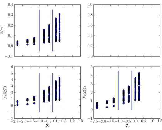
The clustering of the SCG galaxies on the sky is optimal for the narrow FOV spanned by CINDERS and the minimum spacing of the probes (100 arcseconds). CINDERS spectra could provide a two dimensional distribution of age, metallicity, SF and AGN emission in the central regions of these galaxies. The Lick indicesM g2 and< F e >could map the age and metallicity of the stellar populations that fall in our fibers. When combined with the Balmer absorption lines (Hδ, Hγ, Hβ ) which trace star formation in the last Gyr, tighter constraints could be put on the ages of the populations and the SFH of the galaxy. Older ages show that SF has ceased in a galaxy but high metallicities would indicate rapid processing of elements via enhanced SF due to an abrupt compression of cold gas. Any current or recent SF in the last 107 yrs could be traced byHαemission in our maps. Strong emission line ratios ([OIII]5007/Hβvs [NII]6583/Hα) can classify the type of activity occurring in each fiber. If group membership influences central activity, the central regions SCG galaxies should cluster in areas of a Baldwin, Phillips & Terlevich (BPT) diagram distinct from field galaxies. Central regions showing enhanced SF compared to field galaxies could indicate that the groups are undergoing a merger scenario as described by Kauffmann et al. 2004. Measured SF that is lower than in field galaxies could indicate diminishing of SF in the massive halo scenario. If SF is the same then either the dark matter halos of the galaxies in the compact groups have not merged yet or we are seeing an intermediate stage following a period of enhanced SF.

The observations would also map kinematics of gas in the central regions. This could determine how much external factors perturb gas motions in the central regions. Gas funneled into the center of the galaxy would trigger circum-nuclear SF, which would show up inHα emission maps.

(38)

2.2: Extra-galactic Stellar Populations

2.2.1: History of Stellar Population Analysis

Within the Milky Way, astronomers can study the spectra of individual stars to uncover the chemical signatures of past star formation. For galaxies outside the Local Group, it is impossible to see individual stars. Astronomers must use evolutionary population synthesis techniques to unmix stellar populations in a galaxy’s spectrum. This method requires theoretical stellar evolution tracks that populate a Hertzsprung-Russell (HR) diagram with a simple stellar population (SSP). An SSP is a population of stars that were all born at the same time with the same initial chemical composition. A series of SSPs can be used to approximate a galaxy’s star formation history.

Figure 2.1: Color versus age for three types of metallicity[106]. Higher V −I values correspond to redder colors.

(39)

Figure 2.2: Theoretical HR diagrams from [107]. Tracks follow how the luminosity and temperature of a star at a given mass changes throughout its lifetime. The plot on the left is for low mass stars and the plot on the right is for intermediate mass and massive stars. Stars in both plots have compositionY = 0.230 and

Z= 0.0001. The mass of each star is indicated in solar masses next to each curve.

(40)

Figure 2.3: Isochrones derived from theoretical HR diagrams by [107]. Ages span from log(age/yr) = 6.8−10.2 in intervals of 0.2.

The initial mass function (IMF), defines the number of stars born with masses betweenm+dm. There are four commonly used IMFs[116]. The first two are the unimodal and bimodal IMFs. The unimodal is a simple power law whereα= 1.35 is the Salpeter IMF[117] defined for the solar neighborhood.

Φ(m) =βm−α 0.4< m

M

<10 (2.1)

The bimodal IMF is based on observations of Scalo, 1986 and theoretical work of Kroupa et al. 1993[118, 119]. It combines different power laws for different mass ranges. Theαvalues for the mass ranges are

Φ(m) =               

0.035m−1.3 ₀_.₀₈_≤ m M <0.5

0.019m−2.2 0.5≤ m M<1.0

0.019m−2.7 1.0≤ m M

(2.2)

(41)

Original:

Φ(m)∝               

m−0.3 0.01≤ m

M <0.08

m−1.3 0.08≤ m M <0.5

m−2.3 0.5≤ m M

(2.3)

Revised:

Φ(m)∝                       

m−0.3 0.01≤ m

M <0.08

m−1.8 0.08≤ m M <0.5

m−2.7 0.5≤_Mm

<1.0

m−2.3 1.0≤_Mm

(2.4)

The final piece is observed template stellar spectra at various determined effective temperatures, surface gravities, and metallicites, which are used to assign spectra to stars at the different evolutionary stages on the HR diagram. The integrated flux of all of these stars mimics the spectral energy distribution (SED) of this stellar population and is given by

Fλ(t, Z) =

Z Mu

Ml

fλ(M, t, Z)Φ(M)dM (2.5)

whereF_λis the flux per wavelength of a population of agetand metallicityZ, the limits of the integration are over the range of masses defined by the IMF (Φ(M)) andfλ is the flux per wavelength of a given spectrum

(42)

Figure 2.4: Table 1 from [123] which lists the properties of the most commonly used stellar templates.

From these SSPs one can measure expected values of strong absorption lines to obtain model predictions. These predictions are then compared to the measured indices in an observed spectrum. The lines used most often for this are the 25 Lick/IDS lines, which use as models 460 stars with a wide range of atmospheric parameters but at low resolution and signal to noise[124, 125, 126, 127, 128]. There are few young, hot stars in this library, so these lines are adequate for early-type galaxies with older populations[122]. The observed spectrum must be broadened to the Lick/IDS resolution, which degrades the original high resolution spectrum considerably.

Evolutionary population synthesis techniques allow observers to retain high resolution spectra by using the SSP libraries to fit an entire observed SED for a given galaxy. There are now extensive libraries of SSPs [122, 116] and many codes that search parameter space for the best combination of SSPs that match the observed spectrum[129, 130, 131, 132, 133]. These techniques have been applied to galaxies in a wide range of environments. I focus on the results of stellar population analysis of compact group galaxies.

2.2.2: Compact Group Stellar Populations

(43)

More recent studies show that HCGs have higher rates of old and intermediate stellar populations than field galaxies, especially those galaxies classified as early-type[135]. Galaxies classified as late-type are more likely to have similar ages to field galaxies, again, pointing to enhanced processing of cold gas in more evolved galaxies[136, 48, 135, 137]. The elliptical galaxies in HCGs have enhanced [M g/F e] ratios and depleted [Z/H], suggesting that the cold gas was quenched to truncate the star formation[48].

2.2.3: STARLIGHT

My stellar population analysis used the STARLIGHT routine[130]. STARLIGHT fits a spectrum syn-thesized from many template stars to an observed spectrum, to constrain properties of the SP; it uses a combination of simulated annealing, Metropolis and Markov Chain Monte Carlo techniques. There are four steps to the fit. The first explores the parameter space. The second removes pixels that cannot be fit. The third attempts a fit using all the bases provided. The final step tweaks the fit after discarding bases that do not make a significant contribution.

The many parameters to set are discussed in the manual available on the STARLIGHT website. I used the suggested values for my fits. STARLIGHT outputs a very detailed file that includes the normalized input spectrum, the model, and the percent light and stellar mass contributed from each base.

Fit Analysis

(44)

Figure 2.5: MILES metallicity properties plotted over the Padova isochrones. MILES covers the lower main sequence and RGB phases at both metallicities.[139]

There are complications in using the MILES (and other spectral libraries) that are extensively covered in Conroy (2013), and mentioned briefly here. Coverage of the spectra in age, metallicity and regions of the HR diagram, while better, are still not sufficient. The lack of hot, low-metallicity stars makes young ages difficult to fit. There are issues when assigning stellar physical parameters to the stars in the libraries. The errors associated with log g,Tef f and [F e/H] propagate into the SSP models in a significant way. Finally,

(45)

Figure 2.6 shows examples of the MILES spectra used as base templates in STARLIGHT. Because these spectra are flux calibrated, for each template I took 10%, 30%, 50%, 70% and 100% of the light and added Poisson noise of 10, 20 and 30. This procedure is similar to that of Fernandes et al. 2005[130] hereafter referred to as F05. As my priors, I combined two populations, an old+intermediate population and an old+young population. Each population was taken at 50% and added to the other along with the noises applied to the single population. Finally, I combined an old, intermediate and young population each taken at 33% and added the noise. The populations all had the same metallicity, and the ages were chosen at random.

Age and Metallicity Bins

I first used the fits to the single population templates to define my output age and metallicity bins. To explore where the age and metallicity ranges might fall, I plotted the template ages and metallicities against some commonly used Lick indices measured by MILES.

(46)

From this plot, I decided to vary the maximum value for the young SP range from 0.1 to 1.5 Gyrs. The output ages and percent light values were averaged for all templates that fell in the young age ranges. I then calculated the light weighted (xj) and mass weighted (µj) ages and metallicities as suggested by F05.

<logt∗>L=

X

j

xjlog10tj (2.6)

<logt∗>M=

X

j

µjlog10tj (2.7)

< Z >L=

X

j

xjZj (2.8)

< Z >M=

X

j

µjZj (2.9)

Light weighted ages are expected to represent the younger populations because a galaxy’s light will be dominated by younger stars. Mass weighted ages trace the older stars. I subtracted these averaged values from the input values and determined which maximum value for the range returned the smallest deviation from the input value. This analysis determined that the young range should run from Age <0.1 Gyrs. I then used this age as the lower end of the intermediate age bracket and varied the maximum value from 1.7 to 4 Gyrs. From this analysis, the intermediate age was found to range from 0.1≤age≤4.0 Gyrs. The old age range was found to beage >4.0 Gyrs.

(47)

I followed a similar procedure for the metallicity bins. The plots of the Lick indices revealed that the values were already separated into three distinct ranges.

Figure 2.9: Z vs Lick indice for 294 MILES templates. Blue vertical lines indicate where the low, mid and high Z bins are located.

When running the analysis, I varied the maximum of the low and mid ranges. Metallicities did not separate into brackets as cleanly as ages, most likely due to the large spacing between the different metallicity values. A more continuous distribution would allow for better testing. Here I used the visually apparent bins. My results are tabulated in Appendix A.1.

STARLIGHT Fits

(48)

bin (in bold) and also kept the templates for the other metallicities. The following templates were used in my analysis.

Age (Gyr) 0.0631, 0.0794, 0.1995, 0.5012, 1, 2.5119, 6.3096, 10 Z [M/H] ,-2.32,-1.71,-1.31,-0.7,-0.4,

0.00,0.22

Table 2.1: Templates used for analysis.

I used these templates to fit the one, two and three population spectra. I then compared the different population fits with all 294 templates, the bolded 24 templates and the full 56 templates. When looking at the residuals (agein−ageout;Zin−Zout) there is not a substantial difference between the single population

fits and the mixed population fits. This is noted by the tables in Appendix A.2, which list the average and standard deviations of the residuals for each template fit. I also included tables of the residuals over all the files, only separated by number of templates and noise in Appendix A.3.

For the young populations (tj <0.1 Gyrs), the light weighted output ages were on average 0.07 dex

younger than the input ages and did not vary with noise or templates used. For the old populations (tj>4.0

Gyrs), the mass weighted output ages were older than the input ages by 0.06 dex for the 294 template fits. The difference was 0.13 dex for the 24 and 56 template fits.

The intermediate populations (0.1≤tj≤4.0 Gyrs) presented a challenge. My fits were showing very

(49)

Number Fit Number Not Fit

Total 2878 9956

% Total 22% 78%

% Light

10% 439 1577

30% 876 3093

50% 649 2168

70% 452 1564

100% 462 1554

Number of Templates

24 5 4273

56 7 4343

294 2866 1340

Input Noise

10 1117 3161

20 964 3314

30 797 3481

Table 2.2: Total templates fit and not fit by intermediate populations.

My data analysis had to take this into account. There are a few ways to do this: 1) I noted which fits only return young and old populations and calculated the total light weighted average age, 2) I noted which fits only return young and old populations and re-fit the spectrum with a base of only intermediate populations, and 3) I added more intermediate population templates to my base to see if this resulted in more intermediate templates being used.

For the Z analysis, the results were similar for the metallicity brackets and populations. I did not create as many different mixed populations as with the age templates. This could have affected the mixed population residuals. The residuals were similar between the single population Z residuals and the mixed populations that had more than a few files in that Z bracket. I created the same tables as for the age analysis in the Appendix.

(50)

Comparison With Other Data

I carried out long slit observations of an early and a late-type galaxy whose central 1” regions were fit with STARLIGHT by Cid Fernandes et al. [140] (hereafter CF04). They used galaxies with known stellar population properties as their templates. They had four different classifications for their templates:

• NGC 3367 and NGC 6217 are galaxies with young (<107Gyr) populations. Their spectra have weak metal absorption lines and the continuum is blue dominated.

• NGC 205 is a galaxy in the intermediate age range (108−109_Gyr_{). High order Balmer absorption lines} (HOBLs) dominate the spectrum.

• NGC 221 and NGC 628 are galaxies with a mix of intermediate and old populations. The spectra show a mix of HOBLs and strong metal lines.

• NGC 224, NGC 1023, NGC 2950 and NGC 6654 are dominated by old populations and show strong metal lines.

After fitting the central 1” of NGC 660 and NGC 1052, they determined the percentage of light each population contributed to the observed spectrum. Their analysis revealed that NGC 660 is mostly comprised of intermediate (59.4%) and old (40.6%) populations. While NGC 1052 is dominated by older populations (83%) but has a small population of young stars (16.5%) in its central regions. My observations used the age bins described previously and the MILES templates. I fit using 56 and 294 templates to see if that had a significant effect on the outcome. Because I used different templates as my bases, I expected to match their percentages only broadly. As evident in the table below, my fits generally matched those of CF04 in stellar population characteristics.

Galaxy NGC 660 NGC 1052

Templates CF04 56 294 CF04 56 294

% Young 0.0 7.8 5.9 16.5 8.6 7.1 % Intermediate 59.4 75.3 76.5 0.0 0.0 1.0 % Old 40.6 11.3 13.1 83.0 98.0 97.3

(51)

In these two examples, it appears that using more templates recovers a slightly higher percentage of interme-diate aged populations. This should be analyzed in future work to determine how sensitive the intermeinterme-diate aged fits are to the number of templates used.

Future Work

More analysis should be done to ensure that STARLIGHT is accurately recovering the intermediate aged populations. This would require galaxy spectra with known stellar population properties to find the best combination of templates, then cycle through various combinations of templates to find the best match.

2.3: Emission Line Fitting

2.3.1: History of Emission Line Measurements

Emission lines in the optical spectra of galaxies are caused by two phenomena. When gas is photoionized by young stars, Balmer lines are visible. The nucleus of a galaxy will show signs of activity when gas is funneled into the supermassive black hole at the center to cause forbidden lines such as [OI], [OII], [OIII], [NII] and [SII] to appear at differing intensities depending on the nature and orientation of the nucleus. AGN can be further divided into Seyfert and LINER nuclei. LINERS have lower luminosities than Seyferts and are believed to be caused by shock heating due to star formation outside the nucleus or a heavily extinguished AGN[141].

(52)

Galaxies tend to fall into three categories of activity - star forming, AGN, or neither. BPT diagrams can divide galaxies by their activity[142]. These diagrams utilize the ratio of emission from forbidden line phenomena and star forming, most commonly [OI]/Hα, [SII]/Hα, [N II]/Hα and [OIII]/Hβ. These diagrams were revised by Osterbrock & Pogge, 1985 and Veilleux & Osterbrock, 1987 to further constrain the activity types[143, 144]. Diagram divisions based on theoretical models were first proposed by Kewley et al. 2001 with further modification to include composite galaxies in Kauffman et al. 2003[145, 7]. The division between Seyfert and LINER activity is best defined by the classifications in Kewley et al. 2006[141]. We present the definitions of Kewley et al. 2006 here.

Star forming:

log([OIII]

Hβ )<

                

0.61

log([N II_Hα])−0.05+ 1.3 0.72

log([SII_Hα])−0.32+ 1.30 0.73

log([_HαOI])+0.59+ 1.33

(2.10)

Composite/Transition:

0.61

log([N II_Hα])−0.05