Sharif University of Technology
Scientia IranicaTransactions E: Industrial Engineering www.scientiairanica.com
Optimization of weighted correlated multiple responses
using a probabilistic index
M. Bashiri
and M.H. Bakhtiarifar
Department of Industrial Engineering, Faculty of Engineering, Shahed University, Tehran, Iran. Received 25 September 2014; received in revised form 11 May 2015; accepted 15 June 2015
KEYWORDS Cardinal weight; Ordinal weight; Multiple-response optimization; Correlation; Transformation.
Abstract. Dealing with more than one response in the process optimization has been a great issue in recent years; therefore, multiple-response optimization studies have grown in the published works. In the common problems, there are some input variables which can aect output responses, but optimization can be more complex and more real when the responses have correlation with each other. In such problems, the analyst should consider the correlation structure in addition to the eects of input variables. In some cases, response variables may emerge by dierent distributions from the normal ones, which can be analyzed by the proposed method. Moreover, in some problems, response variables may have dierent levels of importance for the decision maker. In this study, we try to propose an ecient method to nd the best treatment in an experimental design, which has dierent weights for correlated responses ,either cardinal or ordinal. Also, a heuristic method is proposed to deal with problems that have a considerable number of correlated responses, or treatments. The results of some numerical examples conrm the validity of the proposed method. Moreover, a real case of air pollution in Tehran is studied to show the applicability of the proposed method in the real problems.
© 2016 Sharif University of Technology. All rights reserved.
1. Introduction
In recent years, due to the growth of industry and need to consider more than one output in the experiments, multiple responses optimization has been discussed in many articles. Accordingly, several methods have been proposed to optimize problems with multiple quality characteristics. Each method has its properties and the analyst should choose the best approach with regard to the problem issue. In some problems, all the responses have the same value for us and nding the best treatment will not be a very dicult problem. On the other hand, there are so many multiple-response problems with dierent levels of response importance in the real world cases. In these problems, a response
*. Corresponding author. Tel.: +98 21 51212092; Fax: +98 21 51212020
E-mail address: [email protected] (M. Bashiri)
may be more important for the analyst than others and the analyzer may be interested in nding the values of controllable factors with the least deviation from the more important response target.
By study of the literature, it can be seen that there are many methods to optimize multiple-response problems when each response has a weight. But, in most of them, the correlation between responses have been ignored. For example, Jeyapaul et al. [1] used the genetic algorithm to obtain weights for each response and optimized them. However, they assumed that re-sponses were independent from each other. Chiao and Hamada [2] proposed a probabilistic method to study problems with correlated responses, but there is a ques-tion about the interpolating weights of each response in such method. Maghsoodloo and Chang [3] developed the quadratic loss function and signal to noise ratio for a bivariate response when both quality characteristics were from the same type. They interpolated social
quality loss for each response to consider the impor-tance of each quality characteristic. Maghsoodloo and Huang [4] focused on mixed bivariate responses and developed quadratic loss function and signal to noise ratios for them. Ozdemir and Maghsoodloo [5] extended quadratic quality loss function and signal to noise ratios for trivariate cases. Wu [6] proposed a method by considering the double-exponential desir-ability function, which has been modied based on Taguchi's loss function, to nd the optimum values for correlated multiple quality characteristics. Ko et al. [7] suggested a new loss function method to accommodate robustness, quality of predictions, and bias in a single framework. Importance of each response was not considered in this approach. Some studies used Principal Component Analysis (PCA) to transform correlated responses to independent ones and then performed optimization. Antony [8] used only the rst PC, but Liao [9] considered all PC's and proposed weighted principal component method. Datta et al. [10] performed PCA method and then utilized the genetic algorithm. Hejazi et al. [11] applied goal programming to model and optimize multi-response surfaces. They used group decision making to obtain the weights of response variables. In many publications, articial neural network has been used to estimate values of responses for non-performed treatments. For example, Noorossana et al. [12] used an articial neural network to estimate the quantitative and qualitative response functions and then performed the optimization step by using genetic algorithm. Salmasnia et al. [13] used neuro-fuzzy and PCA to make a desirability function to optimize correlated multiple responses. Bashiri and Bakhtiarifar [14] proposed an optimality probability index to choose the best treatment in an experimental design with correlated normal responses. With regard to this information, it can be concluded that there is lack of an appropriate and practical method which can consider both cardinal and ordinal importance of correlation structure and responses.
Dealing with non-normal multivariate responses can be very problematic for most researchers. To simplify these problems for analysis, a transformation can be applied to normalize non-normal responses. Niaki and Abbasi [15] transformed multi-attribute data in a way that their marginal probability distributions had almost zero skewness. Riani [16] introduced alternative tests which did not require the maximum likelihood estimates of the transformation parameters. Review of previous works shows that a compre-hensive study on the multiple correlated non-normal responses optimization with dierent response weights does not exist; therefore, this study attempts to propose a method to consider the mentioned problem. To show the eciency of the proposed method in real
cases, an example about the air pollution problem of Tehran is studied.
The next section contains the proposed method, which starts with model statement in three cases of responses without weights, cardinally weighted re-sponses, and ordinally weighted responses for normal and non-normal ones. Then, estimation of the needed parameters is explained in Section 3 and afterwards, a heuristic algorithm is presented to nd the optimum treatment using the proposed indices in Section 4 section. In Section 5, some numerical examples of dierent cases and a real problem are given for better illustration of the proposed approach. Finally, the last section includes the conclusion and future research directions.
2. Proposed method
The aim of this method is to extend the optimality probability index, which has previously been proposed by Bashiri and Bakhtiarifar [14]. The presented index tries to nd the best treatment by calculating its optimality probability in comparison with other treatments. In their proposed index, it is assumed that all responses are normally distributed while there is no a priori information of responses. In real cases, we deal with non-normal responses while some of them are more important than others; therefore, in this study, the optimality index is extended to be calculated in more real situations. The proposed method is explained for both normal and non-normal cases in three states of response importance. In a nutshell, the contributions of this paper, compared to Bashiri and Bakhtiarifar [14], can be mentioned as the ability of incorporating cardinal and ordinal weights as well as considering non-normal distribution for correlated responses.
2.1. Normally distributed responses
Suppose that we have an experimental design with n treatments and m normally distributed correlated responses. We interest to nd the best treatment to achieve optimum values for the responses. To do this, we dene a multivariate probability for each combination which shows the probability of being op-timum in all responses between all the treatments. As mentioned before, the proposed method is considered in three states of non-weighted, cardinally weighted, and ordinally weighted of responses, which are described in the following subsections.
Each response can be of a Smaller The Better (STB), Larger The Better (LTB), or Nominal The Best (NTB) type. In the case of STB responses, it is obvious that a treatment which has smaller values can dominate another one with larger values of responses. We can state this by dening a probability measure as stated
below:
P Ik;i= P (y1k < y1i; :::; ymk< ymi) ; (1)
where P Ik;i is the probability that kth treatment is
better than ith treatment and ymi is the mth response
value corresponding to the ith treatment.
To nd the best treatment, the analyzer should nd the Optimality Probability Index (OPI) proposed by Bashiri and Bakhtiarifar [14] for each treatment as follows:
OPIk= n
i=1 i6=k
P (y1k< y1i; :::; ymk < ymi); (2)
where OPIk is the optimality probability index of kth
treatment.
Similarly, we can nd OPI for problems with LTB-type responses. In such problems, the best treatment should have larger response values than other treatments. In the case of NTB responses, we need to nd absolute target corrected values for each response in each treatment. The treatment with the minimum absolute deviation value from its target is our favorite one. The OPI for the kth treatment is product of probabilities that shows k is better than other treatments:
OPIk= n
i=1 i6=k
P jy1k t1j < jy1i t1j; :::; jymk tmj
< jymi tmj; (3)
where ymiis the mth response corresponding to the ith
treatment and tmis target value for the mth response
when its type is Nominal The Best (NTB).
The multivariate probability function of absolute deviation for NTB responses can have another distribu-tion rather than the normal one. So, calculating Eq. (3) may be very dicult. To solve this problem, we can transform NTB responses into STB-type by using the deviation terms as new variables. This transformation can violate the normality assumption. So, we should use another transformation on new STB values to change their distribution into the multivariate normal one.
In some cases, when we deal with some responses with dierent types, for example when the problem has some LTB and STB responses, we can use negative values for LTB-type response(s) to transform them into STB or use a mixed multivariate probability which can be obtained by changing Eq. (2).
2.1.1. Multiple responses without weights
In case of responses with the same importance, the proposed Bashiri and Bakhtiarifar's OPI [14] can be used. Moreover, other methods from literature, such as Chiao and Hamada [2], can be utilized as well.
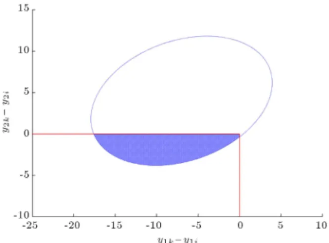
Figure 1. The condence region for the mentioned probability.
2.1.2. Multiple responses with cardinal weights In some problems, responses have dierent levels of importance for the analyzer. It means that one or more responses may be more attractive than the others. In these cases, we cannot use the previous equations to nd the best treatment, because the importance of responses has been ignored in the OPI index. So, weights of responses should be considered in a new developed optimality index.
For better comprehension, describing an example can be helpful. Suppose that there is an experimental design with two correlated normal STB-type responses. The mean array of the responses for the kth treatment is computed as [3 5], while it is equal to [10 1] for the ith treatment. The covariance matrix of the responses in both of the treatments is equal to
10 2
2 5:1
. Figure 1 illustrates the 95% condence region for P (y1k <
y1i; y2k < y2i).
It can be concluded that the kth treatment has better value in the rst response, but worse in the second one. In this situation, we expect that allocating greater weight to the rst response would increase the desired probability while allocating greater weight to the second response would decrease it. At rst, we transform the weights through dividing them by the minimum weight. Then, we perform a t-test for each response. If the test shows that treatment k has better value in the nth response, then we multiple yniby the
corresponding transformed weight; but if the test shows that treatment k has worse value in the nth response, then we multiple ynkby the corresponding transformed
weight. Therefore, in the mentioned example, the weighted probability for treatment k to be better than treatment i; WPIk;i is calculated as follows:
WPIk;i= P (y1k< w1y1i; w2y2k < y2i) ; (4)
where wjis the transformed weight of the jth response.
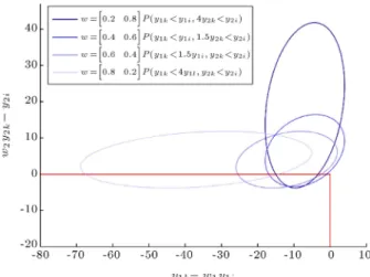
Figure 2. The condence regions for the WPIkibased on
dierent weights.
equal weights. Figure 2 shows various 95% condence regions based on dierent weights for WPIk;i in the
mentioned example.
In the case of LTB and NTB responses WPIk;i is
obtained by the same logic. Therefore, the Weighted Optimality Probability Index (WOPI) for the kth treatment can be computed by multiplying WPIs as follows:
WOPIk = n
i=1 i6=k
WPIk;i: (5)
2.1.3. Multiple responses with ordinal weights
In case of ordinal weights, we deal with responses which have dierent levels of importance dened by ranks. It means that order of the responses shows the importance of them. It is clear that in such cases, we do not have cardinal weight value for each response to nd weighted optimality probability like the aforementioned equations. In this situation, we should consider responses ranking in the optimality probability calculation. For better comprehension, suppose that all of the responses are of the STB type. First, we sort responses based on their importance in a descending order and put them in a set named J. Then, to nd the Ordinal Optimality Probability Index (OOPI) for the kth treatment, we should calculate the probability of the kth treatment to have a smaller value for J(1) response as the most important response versus other possible treatments. If the most important response (J(1)) value for the kth treatment is statis-tically equal to its value in the ith treatment, then we should nd the probability for the kth treatment to have a smaller value of J(2) than that of the ith treatment, and so on. Therefore, to nd OOPI, we need to perform a t-test to verify the hypothesis of equality of J(1) values for the treatment and other ones. If the equality cannot be rejected, then another hypothesis test should be done on J(2) value, and so
on. After selecting the proper response based on this method, the eect of other responses from the measure should be eliminated. To do this, we nd proper weight coecients, wj, for other responses such that
the equality t-test on them in two compared treatments cannot be rejected and it has an enough great p-value. Note that the placing side of weight coecients should be selected based on the explanations in the previous subsection. For better understanding, consider the example with two STB correlated responses in the previous subsection. The hypothesis t-test on the equality of y1k and Y y1i is rejected by a near zero
p-value. Therefore, we should nd a proper weight for the second response to eliminate its eect in the proposed measure as follows:
OPk;i= P (y1k < y1i; w2y2k< y2i) : (6)
By iterating these steps for all other treatments, the OOPIk can be calculated as follows:
OOPIk= n
i=1 i6=k
OPk;i: (7)
2.2. Other multivariate distributions
Suppose that the response values have another mul-tivariate distribution rather than the normal one. In such problems, an idea is using a transformation to normalize responses before optimization stage. In this paper, NORTA inverse method, proposed by Niaki and Abbasi [17], is used to transform correlated values into normal ones. For better comprehension, consider normal to anything (NORTA) method (Cario and Nelson [18]) which can generate a k-dimensional random vector X where Xihas an arbitrary cumulative
distribution function FXi with correlation matrix. In this situation, a transformation on a k-dimensional standard multivariate normal vector Z with correlation matrixPz should be performed to generate vector X as follows:
X = 0 B B B @
FX11[(z1)]
FX21[(z2)]
... FXk1[(zk)]
1 C C C
A; (8)
where is the cumulative distribution function of a univariate standard normal. To nd the correlation between Xi and Xj, the following equation should be
solved for each pair of variables: E(XiXj) = E
F 1
Xi [(zi)] F
1 Xj [(zj)]
= Z +1
1
Z +1
1 F 1
Xi [(zi)] F
1 Xj [(zj)] 'z(i;j)(zi; zj)dzidzj: (9)
Since these equations are usually unsolvable for many marginal distributions, Cario and Nelson [18] presented some theorems to help researchers do this. As another alternative, the simulation can be used to estimate the covariance matrix.
By such descriptions, as can be deduced, the NORTA inverse method transforms a vector of multi-attribute variables such that they have multivariate normal distribution. The following formula is used for this purpose:
Y = [Y1; Y2; :::; Yk]T =
1(F
X1(x1)) ;
1(F
X2(x2)) ; :::; 1(FXk(xk)) T
: (10)
Thereafter, the covariance matrix of the generated normal attributes is estimated through the simulation. 2.3. Parameter estimation
In order to calculate the previous equations, we should estimate parameters for multivariate normal distribu-tion, in each treatment. To do this, regression can be used for each parameter when the hypothesis of its normality cannot be rejected. Eq. (11) shows multi-variate normal distribution where Y = [y1; y2; :::; ym],
M = [1; 2; :::; m], andP= byiyjc (i = 1; 2; :::; m; j = 1; 2; :::; m) are response vector, mean vector, and covariance matrix, respectively:
f(y1; y2; :::; ym)= 1
(2)m2jPj12e( 1
2(Y M0)P 1(Y M)); (11) where jPj is determinant of covariance matrix and (Y M)0 is transpose of (Y M). As can be seen, we
need to estimate mean and variance for each response and covariance for each couple of responses in each treatment. The least square estimators are as follows:
^i= xi; i = 1; :::; m; (12)
log(^2
i) = xi; i = 1; :::; m; (13)
tanh 1(^
ij) = xij; 1 i j m; (14)
where x is a row vector of controllable variables and i, j, and ij are the column vectors that their
com-ponents determine the impact of associated variables. To ensure positive values for variances, logarith-mic model is used. On the other hand, as correlation coecients should be between -1 and 1, we use the inverse hyperbolic tangent transformation [19], which is dened as:
tan 1() = 1
2log (1 + )
(1 ): (15)
Weighted optimality probability index can be
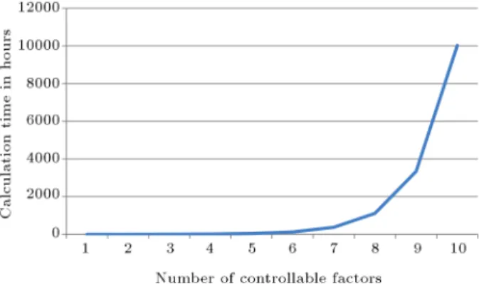
cal-Figure 3. Computational time against the number of controllable factors.
culated for each possible treatment with respect to other treatments by estimating these parameters for responses corresponding to each treatment.
In the case of non-normal parameters, articial neural network can be a good method to estimate parameters for any possible treatment. Note that the number of neurons can change with regard to each design.
2.4. The proposed heuristic algorithm
Calculation of WOPI or OOPI for all possible factor-level combinations may be very time consuming, espe-cially when we deal with sizeable number of responses and controllable factors.
For better comprehension, suppose that we want to calculate WOPI for some problems with dierent numbers of controllable factors. Figure 3 shows esti-mation of computational time to solve such problems on a notebook with an AMD E-350 processor and 4 gigabytes of RAM when all factors have 3 levels. To estimate the computational time, the algorithm was performed for few numbers of controllable factors and then, the computational time was estimated for large numbers of factors using the regression.
It can be seen that by increasing the number of factors, calculation time increases exponentially. So, a heuristic algorithm can be useful to reduce computational time. As another solution for the dominating time problem, we can use an articial neural network. At rst, we need to calculate WOPI for some treatments to train our network. Then, we can use the trained ANN instead of WOPI equation, but it is clear that this approach may cause non-negligible errors.
The proposed heuristic algorithm tries to nd the most probable treatment in each iteration of prob-ability calculation. By this approach, the solution space decreases in each iteration and, consequently, the number of calculations can be reduced. The proposed approach is described in Table 1 as pseudo-code.
Note that the proposed heuristic approach can be extended for problems with ordinal weights as well.
Table 1. Pseudo-code of the proposed heuristic algorithm to nd the best combination. Transform all responses to STB type;
Find the estimation equations for the parameters of multivariate normal probability or train ANN to estimate responses; Select a random factor-level combination k;
Calculate multivariate normal probability parameters for responses in combination k; Calculate WOPIk;
Set k= k, and WOPI= WOPI k;
Set the number of desired combinations to check l;
Select l combinations with minimum WPIk;j values and store in J;
repeat
for k = J(1) to J(l)
Calculate multivariate normal probability parameters for responses in combination k; Calculate WOPIk;
If WOPIk> WOPI, set k= k and WOPI= WOPIk;
Next k;
Select l combinations with minimum WPIk;j value and store in J;
Until WOPIdoes not change.
3. Numerical examples
In this section, two numerical examples from the previous articles are studied according to the proposed method and the results are compared with results of the reference articles. Then, a simulated numerical example with large number of factors is presented to show eciency of the proposed heuristic algorithm. 3.1. Example 1
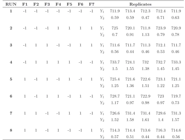
As the rst example, consider an experimental design described by Chiao and Hamada [2]. The goal is to minimize the imbalance of a plastic wheel cover the component when we deal with two NTB quality characteristics: total weight (Y1) and the balance of the
component (Y2). There are seven controllable factors
with two levels which have eect on balance of the component. Table 2 shows the values of two correlated responses in the 8 runs.
The rst step is using Johnson transformation [20] to change NTB responses into STB-types in order to use the proposed method as mentioned in Section 2. Eqs. (16) and (17) show the proper transformations for two responses and as can be seen, Z1 and Z2 are
transformed into STB-type responses: Z1=0:387228 + 0:365089
Ln
jY1 1j 0:0888751
21:2924 jY1 1j
; (16)
Z2=0:122266 + 0:389592
Ln
jY2 2j 0:0863844
1:26185 jY2 2j
: (17)
Now, the least square estimators can be written for multivariate distribution parameters using Eqs. (12)-(15) as follows:
^1= 0:079 0:288x4+ 0:643x5 0:297x7;
^2= 0:047+0:109x3+0:241x1+0:763x5 0:486x7;
log(^2
1)= 1:060 0:390x1+0:202x4 0:267x7;
log(^2
2)= 0:870 0:282x2;
tanh 1(^
1;2)= 0:106+0:559x1 0:318x5 0:494x7:
(18) Table 3 shows three best factor-level combinations for this example. It can be concluded from Eqs. (18) that factor F is not signicant and can be ignored in the estimation of parameters. The optimal combination by the proposed method is (-1,-1,-1,-1,-1, ,1) with optimality probability index of 0:2326 10 12, where
an insignicant factor has been denoted by \ ". To ensure that our proposed WOPI can nd the true order of treatments, we can consider the same weights for responses and use Eq. (5) to calculate WOPI's. Moreover, the proportion of conformance, proposed by Chiao and Hamada [2], is calculated. It can be seen that the OPI and WOPI results are the same.
Now, suppose that the rst response is important for us. Therefore, we deal with a multi-response op-timization problem with ordinal response weights. As described before in section 2, to nd the best treatment, we should calculate OOPI for each of them. Table 4 illustrates the rst three treatments with corresponding ordinal optimality probability indices.
Table 2. Responses values in Example 1.
RUN F1 F2 F3 F4 F5 F6 F7 Replicates
1 -1 -1 -1 -1 -1 -1 -1 Y1 711.9 713.4 712.3 712.4 711.9
Y2 0.59 0.59 0.47 0.71 0.63
2 -1 -1 -1 1 1 1 1 Y1 725 720.1 711.8 723.9 720.9
Y2 0.7 0.91 1.13 0.79 0.78
3 -1 1 1 -1 -1 1 1 Y1 711.6 711.7 711.3 712.1 711.7
Y2 0.56 0.44 0.46 0.53 0.46
4 -1 1 1 1 1 -1 -1 Y1 733.7 724.1 732 732.7 733.3
Y2 1.5 1.55 1.38 1.45 1.45
5 1 -1 1 -1 1 -1 1 Y1 725.4 721.6 722.6 723.1 721.1
Y2 1.25 1.36 1.51 1.22 1.25
6 1 -1 1 1 -1 1 -1 Y1 728.7 721.1 722.9 723 719.7
Y2 1.17 0.97 0.98 0.97 0.73
7 1 1 -1 -1 1 1 -1 Y1 726.6 731.4 731.4 729.6 731.3
Y2 1.52 1.58 1.61 1.4 1.57
8 1 1 -1 1 -1 -1 1 Y1 714.3 714.4 713.6 716.3 714.6
Y2 0.57 0.51 0.44 0.44 0.56
Table 3. Weighted optimality probability index versus POC for the best three treatments in Example 2.
A B C D E G POC OPIk Weighted OPIk
-1 -1 -1 -1 -1 1 0.5332 3:4843 10 13 3:4843 10 13
-1 1 -1 -1 -1 1 0.71216 8:6260 10 15 8:6160 10 15
-1 -1 1 -1 -1 1 0.5332 1:1306 10 18 1:1306 10 18
Table 4. The best three treatments with the considered ordinal weights in Example 1.
A B C D E G OOPIk
-1 -1 -1 1 -1 1 3:1880 10 173
1 1 -1 -1 -1 1 5:7665 10 295
-1 1 -1 -1 -1 1 5:1807 10 304
To verify the eciency of OOPI, WOPI with appropriate weights can be used. For this example, if we choose w1and w20.9 and 0.1, respectively, it can
be seen that treatment (-1,-1,-1, 1,-1, ,1) with a WOPI of 4:0041 10 38is the most probable one.
3.2. Example 2
Consider a simulated design which has nine controllable factors with three levels for each of them and two STB correlated responses. In such a problem, because of the number of factors and their levels, using a heuristic algorithm is necessary. Table 5 shows the calculated parameters for each treatment.
The least square estimators for multivariate nor-mal distribution parameters can be found below:
^1=6:518 + 0:494x1 0:271x2 1:758x3
+ 0:447x2
3+ 0:643x5+ 0:337x8x9;
^2=114:104 + 2:241x4 7:825x6 7:822x8
+ 4:587x6x8;
log(^2
1) = 2:011 0:054x1x2+ 0:091x7x9
+ 0:065x8x9;
log(^2
2) = 1:701 0:216x1 0:223x7 0:077x4x6;
tanh 1(^1;2) = 1:132 + 1:165x1x6+ 0:125x2x3:
(19) Solving such problem on a notebook with an AMD E-350 dual-core processor and 4 gigabytes of RAM can
Table 5. The calculated parameters in each treatment for Example 2.
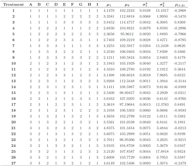
Treatment A B C D E F G H I 1 2 21 22 (1;2)
1 1 1 1 1 1 1 1 1 1 4.1470 102.2243 0.0108 15.1017 -0.2968 2 1 1 1 1 2 2 2 2 2 3.3581 112.8818 0.0068 1.9950 -0.5470
3 1 1 1 1 3 3 3 3 3 3.8452 114.4757 0.0042 6.3085 0.8369
4 1 2 2 2 1 1 1 2 2 2.6830 103.8821 0.0079 8.8593 -0.2996
5 1 2 2 2 2 2 2 3 3 2.3656 95.9612 0.0020 1.8893 -0.7966
6 1 2 2 2 3 3 3 1 1 2.7403 109.2219 0.0028 3.4271 -0.8795 7 1 3 3 3 1 1 1 3 3 4.2255 102.5917 0.0204 15.2438 0.9620
8 1 3 3 3 2 2 2 1 1 3.2540 106.0403 0.0034 7.8308 0.3466
9 1 3 3 3 3 3 3 2 2 2.1211 100.5824 0.0054 2.8403 0.4179
10 2 1 2 3 1 2 3 1 2 3.1943 103.1929 0.0040 1.3277 -0.2117
11 2 1 2 3 2 3 1 2 3 4.3310 109.2780 0.0192 2.1912 0.3644
12 2 1 2 3 3 1 2 3 1 3.1498 106.6018 0.0019 7.9685 0.6525
13 2 2 3 1 1 2 3 2 3 3.9268 112.3448 0.0011 1.3944 -0.3144 14 2 2 3 1 2 3 1 3 1 3.1411 108.5867 0.0073 9.6146 -0.0389 15 2 2 3 1 3 1 2 1 2 3.5400 98.00457 0.0045 3.2939 -0.0311 16 2 3 1 2 1 2 3 3 1 3.6162 107.0205 0.0036 0.6142 -0.9760 17 2 3 1 2 2 3 1 1 2 3.3618 97.19684 0.0013 12.3763 0.8491 18 2 3 1 2 3 1 2 2 3 3.1058 106.5303 0.0060 6.0686 -0.9593
19 3 1 3 2 1 3 2 1 3 4.5658 102.2799 0.0122 1.0111 0.5382
20 3 1 3 2 2 1 3 2 1 3.5561 101.0539 0.0040 6.8441 0.1881
21 3 1 3 2 3 2 1 3 2 4.8375 101.3454 0.0075 3.4844 -0.0213
22 3 2 1 3 1 3 2 2 1 3.6075 103.2989 0.0051 0.0620 0.9199
23 3 2 1 3 2 1 3 3 2 3.7011 96.95306 0.0043 3.2635 -0.9215
24 3 2 1 3 3 2 1 1 3 3.9105 104.8708 0.0003 5.3679 0.0167
25 3 3 2 1 1 3 2 3 2 3.2120 107.8587 0.0044 17.8818 0.9324
26 3 3 2 1 2 1 3 1 3 2.6008 103.7729 0.0004 0.7953 0.5587
27 3 3 2 1 3 2 1 2 1 4.6149 102.5406 0.0093 1.3074 -0.2479 Table 6. Optimality probability for the best three treatments in Example 3.
Rank A B C D F G H I OPIk WOPIk
1 1 3 2 1 3 3 1 1 4:8997 10 128 4:8997 10 128
2 1 3 2 1 3 2 1 1 1:0896 10 144 1:0896 10 144
3 1 3 2 1 3 1 1 1 3:1330 10 169 3:1330 10 169
take much time, i.e. about 3340 hours. Therefore, it is better to use the proposed heuristic approach. By considering 0.5 as weight value for both responses, the proposed algorithm is coded in MATLAB. After about 3823 seconds as computational time, it shows that optimum combination is (1,3,2,1, ,3,3,1,1) with WOPI of 4:899710 128between 6561 possible combinations.
The OPI values conrm our results. Table 6 shows optimality probability values for the best three combi-nations.
3.3. Example 3
Consider a 23full factorial design with three correlated
STB type responses which are generated using NORTA
method. Each treatment has four replicates per each response. Because there is no other possible treatment, we do not need to nd estimators for parameters. Table 7 shows experimental design and response values for this example.
As expressed in Section 2, in such problems, rst, we can use NORTA inverse method to transform multivariate exponential responses into normal ones and then calculate the optimality probability index. Based on the transformed response values, mean, variances and correlation coecients can be calculated for each treatment. Table 8 shows multivariate normal parameters for each treatment.
cal-Table 7. Experimental design with correlated exponential response in Example 3.
Treatment A B C Y1 Y 2 Y 3
1 1 -1 -1 0.08 0.14 0.16 0.22 2.82 5.87 6.45 12.31 55.53 55.74 56.44 62.15 2 1 1 1 0.35 0.39 0.40 0.42 19.34 20.10 23.61 23.95 175.70 177.25 223.08 226.15 3 -1 -1 1 0.54 0.55 0.61 0.89 25.09 33.99 42.37 46.04 307.42 334.23 383.93 386.09 4 1 1 -1 1.00 1.10 1.17 1.19 50.06 56.37 56.60 70.88 399.63 425.76 441.15 487.42 5 1 -1 1 1.25 1.47 1.50 1.88 78.10 87.93 91.01 92.44 600.79 666.50 714.33 806.93 6 -1 -1 -1 2.22 2.31 2.64 2.76 100.75 111.85 116.95 119.34 1035.33 1076.38 1110.87 1240.80 7 -1 1 -1 2.90 3.69 3.92 5.26 137.29 139.16 149.00 164.05 1482.25 1637.67 1689.20 1726.50 8 -1 1 1 5.40 6.66 8.50 16.15 233.06 233.16 255.92 311.97 1762.07 2062.43 3002.15 3641.25
Table 8. Mean, variances, and correlation coecients for normalized responses in Example 3. Treatment 1 21 2 22 3 23 (1;2) (1;3) (2;3)
1 -1.33 0.24 -1.81 0.12 -1.37 0.13 0.98 0.87 0.75 2 -0.75 0.01 -1.28 0.19 -0.70 0.01 0.90 0.96 0.80 3 -0.39 0.03 -0.56 0.00 -0.40 0.00 0.84 0.66 0.92 4 -0.04 0.00 -0.42 0.01 -0.29 0.00 0.80 0.88 0.96 5 0.27 0.00 -0.11 0.01 -0.01 0.01 0.85 0.93 0.96 6 0.45 0.00 0.28 0.03 0.16 0.00 0.98 0.93 0.96 7 0.80 0.13 0.70 0.02 0.93 0.04 0.76 0.87 0.94 8 2.08 0.51 1.67 0.23 1.69 0.27 0.96 0.94 0.95 Table 9. OPI values for each treatment in Example 3.
Treatment OPI
1 0.2887
2 0.0090
3 3:9543 10 8
4 1:3368 10 15
5 2:5850 10 33
6 1:2941 10 61
7 3:0134 10 61
8 2:1035 10 35
culate optimality probability index for each treatment. Table 9 shows OPI for each treatment. It can be seen that the rst treatment is the best factor-level combination by a probability of 0.2887.
3.4. A real case
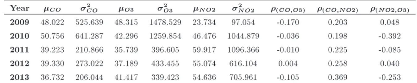
To study the applicability of the proposed method, consider a real case of air pollution in Tehran. Some
of the important factors, including the number of taxies (NTX), the number of minibuses (NMB), the number of bus lines (NLB), the length of Lines for Bus Rapid Transportation in kilometer (LBRT), the length of metro lines in kilometer (LML), the Number of Metro Trains (NMT), and the Number of Metro Stations (NMS), were collected from 2009 to 2013 and are represented in Table 10 (from ocial webpage http://tmicto.tehran.ir). Moreover, three correlated air pollution indices including CO, O3, and NO2 were
gathered in the mentioned period and are illustrated in Table 11 (from ocial webpage http://air.tehran.ir).
The goal is to nd the year with minimum polluted air by considering w = 0:6 0:1 0:3 as weights array. By applying the proposed method, it can be seen that 2013 is the best year with WOPI equal to 5:6864 10 7. As another scenario, r =1 3 2
is selected as order of responses. By calculating OOPI for all years, 2013 with OOPI=0.1656 is selected as the best year. Table 12 shows the WOPI and OOPI results for the years.
Table 10. The values of some important factors of air pollution indices in the dierent years.
Year NTX NMB NLB LBRT LML NMT NMS
2009 70460 1356 359 62.1 106.2 95 64
2010 72370 982 308 85 125 105 70
2011 78857 1442 263 105 129 129 76
2012 77949 1285 246 114.2 140 148 84
Table 11. The mean, variance, and correlation coecients of indices in dierent years.
Year CO 2CO O3 2O3 NO2 2NO2 (CO;O3) (CO;NO2) (NO2;O3)
2009 48.022 525.639 48.315 1478.529 23.734 97.054 -0.170 0.203 0.048 2010 50.756 641.287 42.296 1259.854 46.476 1044.879 -0.036 0.198 -0.392 2011 39.223 210.866 35.739 396.605 59.917 1096.366 -0.010 0.225 -0.085 2012 39.330 273.022 37.189 433.455 55.074 616.104 0.004 0.258 0.040 2013 36.732 206.044 41.417 339.423 54.636 705.961 -0.105 0.369 -0.253
Table 12. WOPI for each year.
Year WOPI OOPI
2009 1:2139 10 8 0.0261
2010 3:8470 10 9 0.0074
2011 4:2432 10 9 0.1284
2012 4:1819 10 9 0.1262
2013 5:6864 10 7 0.1656
Although there are several nuisance factors such as rainfall, wind speed, and temperature inversion which have eect on the air pollution, it can be seen that increase in LML and LBRT as well as decrease in NMB could lead the indices to a better point in 2013. Therefore, based on the results, there is hope that continuing these transportation policies leads to decrease in the air pollution.
Note that there is not any proper alternative method to consider weights as well as correlation struc-ture to compare the results. On the other hand, using methods which have independent viewpoints ignores the correlation structure and thus may lead to a false result.
4. Conclusions
Because of diculty in considering correlated multiple responses in the optimization problems, there are a few studies in this eld. However, such problem would be more dicult when the responses have not the same importance for us. In these cases, the signicance of each response should be interpolated in the model as weights, either ordinal or cardinal. In this paper, we developed a probabilistic index to nd the optimal treatment in an experimental design with normally distributed weighted correlated responses. Moreover, a transformation method from literature was considered to equip the proposed approach to solve the problems with non-normal correlated responses. To show the eciency of the proposed optimality indices, three nu-merical examples were presented. In the rst example, a comparison between OPI, WOPI, and OOPI showed that the results of indices could conrm each other. Moreover, a real case of air pollution in Tehran was studied to clarify the practical aspects of the proposed
method. Other multivariate distributions, such as exponential, gamma, etc. can be considered for future studies.
References
1. Jeyapaul, R., Shahabudeen, P. and Krishnaiah, K. \Simultaneous optimization of multi-response prob-lems in the Taguchi method using genetic algorithm", The International Journal of Advanced Manufacturing Technology, 30(9-10), pp. 870-878 (2005).
2. Chiao, C. and Hamada, M. \Analyzing experiments with correlated multiple responses", Journal of Quality Technology, 23(4), pp. 451-465 (2001).
3. Maghsoodloo, S. and Chang, C. \Quadratic loss functions and signal-to-noise ratios for a bivariate response", Journal of Manufacturing Systems, 20(1), pp. 1-12 (2001).
4. Maghsoodloo, S. and Huang, L. \Quality loss func-tions and performance measures for a mixed bivariate response", Journal of Manufacturing Systems, 20(2), pp. 73-88 (2001).
5. Ozdemir, G. and Maghsoodloo, S. \Quadratic quality loss functions and signal-to-noise ratios for a trivariate response", Journal of Manufacturing Systems, 23(2), pp. 144-171 (2004).
6. Wu, F. \Optimization of correlated multiple quality characteristics using desirability function", Quality Engineering, 17(1), pp. 119-126 (2005).
7. Ko, Y., Kim, K. and Jun, C. \A new loss function-based method for multiresponse optimization", Jour-nal of Quality Technology, 37(1), pp. 50-59 (2005). 8. Antony, J. \Multi-response optimization in industrial
experiments using Taguchi's quality loss function and principal component analysis", Quality and Reliability Engineering International, 16(1), pp. 3-8 (2000). 9. Liao, H. \Multi-response optimization using weighted
principal component", The International Journal of Advanced Manufacturing Technology, 27(7-8), pp. 720-725 (2006).
10. Datta, S., Nandi, G. and Bandyopadhyay, A. \Analyz-ing experiments with correlated multiple responses", Journal of Manufacturing Systems, 28(2-3), pp. 55-63 (2009).
11. Hejazi, T.H., Bashiri, M., Daz-Garca, J.A. and Noghondarian, K. \Optimization of probabilistic mul-tiple response surfaces", Applied Mathematical Mod-elling, 36, pp. 1275-1285 (2012).
12. Noorossana, R., Tajbakhsh, S.D. and Saghaei, A. \An articial neural network approach to multiple-response optimization", The International Journal of Advanced Manufacturing Technology, 40(11-12), pp. 1227-1238 (2009).
13. Salmasnia, A., Baradaran Kazemzadeh, R. and Mo-hajer Tabrizi, M. \A novel approach for optimization of correlated multiple responses based on desirability function and fuzzy logics", Neurocomputing, 91, pp. 56-66 (2012).
14. Bashiri, M. and Bakhtiarifar, M.H. \An optimality probability index for multiple correlated responses", Communications in Statistics-Theory and Methods, 43(20), pp. 4324-4336 (2014).
15. Niaki, S.T.A. and Abbasi, B. \Skewness reduction approach in multi-attribute process monitoring", Com-munications in Statistics-Theory and Methods, 36, pp. 2313-2325 (2007).
16. Riani, M. \Robust multivariate transformations to normality: Constructed variables and likelihood ratio tests", Statistical Methods and Applications, 13(2), pp. 179-196 (2004).
17. Niaki, S.T.A. and Abbasi, B. \Monitoring multi-attribute processes based on NORTA inverse trans-formed vectors", Communications in Statistics-Theory and Methods, 38, pp. 964-979 (2009).
18. Cario, M.C. and Nelson, B.L. Modeling and Generating Random Vectors with Arbitrary Marginal Distributions and Correlation Matrix, Department of Industrial
Engineering and Management Sciences, Northwestern University, Technical Report (1997).
19. Rao, C.R., Linear Statistical Inference and Its Appli-cation, 2nd Ed.: John Wiley & Sons (1973).
20. Choi, Y.-M., Polansky, A.M. and Mason, R.L. \Trans-forming non-normal data to normality in statistical process control", Journal of Quality Technology, 30(2), pp. 133-141 (1988).
Biographies
Mahdi Bashiri is an Associate Professor of Industrial Engineering at Shahed University. He holds a BS degree in Industrial Engineering from Iran University of Science and Technology, MS, and PhD degrees in this eld from Tarbiat Modares University. He is recipient of the 2013 young national top scientist award from Academy of Sciences of the Islamic Republic of Iran. His research interests are facilities planning, metaheuristics, and multi-response optimization. Mohammad Hasan Bakhtiarifar received his BS degree from Imam Hussein University, Tehran, Iran, and MS degree in Industrial Engineering from Shahed University in Tehran, Iran, where he is currently a PhD degree student in the same eld. His research interests include design of experiments, multiple-response opti-mization, multivariate probabilities, and metaheuristic algorithms.