Identication of Inelastic Shear Frames
Using the Prandtl-Ishlinskii Model
M. Farrokh
1and A. Joghataie
1;Abstract. In this paper, a new method is proposed for identication of inelastic shear frame structures with hesteresis, using data collected on their dynamic response. It uses the Prandtl-Ishlinskii rate independent model for hysteresis, which was originally used in the eld of plasticity and ferromagnetism. The proposed identication method is capable of identifying the mass, damping and restoring force of a frame structure, which can be used in forming the equations of motion of the frame. By solving the equations of motion, the dynamic response is predicted. The method is based on the combined use of Quadratic Programming (QP) and Genetic Algorithms (GA). First, assuming a set of Prandtl-Ishlinskii constants, the QP is used to nd the best frame parameters that can be used in its equations of motion to predict its dynamic response with the minimum of error compared to the real data collected on its dynamic response, while the GA is used to nd the best Prandtl-Ishlinskii constants for more reduction in error. The method has been applied to dierent frames with bilinear nonlinearity where the results show the high capability of the method. Two examples, a Single and a Multi Degree Of Freedom (SDOF and MDOF) frame, are included in the paper.
Keywords: Prandtl-Ishlinskii model; Identication; Inelastic behavior; Structural dynamic; Earthquake.
INTRODUCTION
Identication of hysteretic systems is a problem widely encountered in the eld of structural dynamics. For example, the inelastic nonlinear behavior of a structure is usually seen during strong ground earthquake exci-tation. Due to their hysteretic behavior, the restoring forces not only relate to the current state variables, but also to the history of state variables. This phe-nomenon complicates the modeling and identication of hysteretic systems. Many research studies have been reported in the literature about either the modeling or identication of hysteretic systems. Some noteworthy research on this problem are mentioned in Brokate [1], Iwan [2], Bouc [3], Wen [4,5], Benedettini et al. [6], Chassiakos et al. [7], Sato and Qi [8], Smyth et al. [9] and Kosmotopoulos et al. [10].
In this study, the authors have utilized the Prandtl-Ishlinskii model in the equations of motion of shear frames, in order to identify their dynamic
1. Department of Civil Engineering, Sharif University of Tech-nology, P.O. Box 11155-9313, Tehran, Iran.
*. Corresponding author. E-mail: [email protected]
Received 31 May 2006; received in revised form 17 January 2007; accepted 7 February 2007
parameters, such as mass, damping and restoring forces, based on the measurement of displacement, velocity and acceleration at a number of its degrees of freedom, as well as the external excitations. The new identication method also uses the Genetic Algorithm (GA) to nd the Prandtl-Ishlinskii constants. The proposed method has been tested for a number of frames, including Single and Multi Degree of Freedom (SDOF and MDOF) inelastic frames with bilinear nonlinearity, where the results assert the capability of the method. The method has been rstly developed for the SDOF shear frames, but then, generalized to the multi degree of freedom (MDOF) shear frames. As examples, a one story and three-story shear frame, considering a dierent restoring force for each story, have been used in the assessment of the proposed method, where the identication results have been satisfactory.
In the following sections, rst, a brief explanation of the stop operator, the Prandtl-Ishlinskii model and the equations of motion of the SDOF frames, are included. Then, the essentials of identication methods, followed by a brief explanation of the GA, are presented. Finally, the examples and discussion of results are reported.
STOP OPERATOR
Prandtl has introduced an elasto-plastic model called the \stop operator" [11]. The model can be explained by means of a heavy body connected to a spring, which can move freely on a horizontal surface, as depicted in Figure 1a. In this model, the spring stiness is assumed to be:
k = 1: (1)
Denoting x = displacement of point A, z = displace-ment of the body or stop operator drift and, assuming Columb's friction exists between the body and the horizontal surface, the dierential equation of the stop operator is written as follows [11]:
f = x z; (2a)
_z = (
_x for jx zj = r and _x(x z) > 0
0 otherwise (2b)
where f is spring force and r = threshold > 0.
The hysteresis diagram of a stop operator is shown in Figure 1b. The input-output behavior of the stop operator can also be described in analytical form for a given piecewise monotonic input, x. Dening ti = it
and assuming x is monotonic in each interval [ti; ti+1],
then:
f(t) = "r[x(t)]; (3)
where r is Prandtl parameter, dened in Equation 2b, and "r is a symbol representing the stop operator [1],
which is described by induction as:
f(ti+1)=minf r; maxfr; [x(ti+1) x(ti)+f(ti)]g;
(4a)
f(t 1) = x(t 1) = 0: (4b)
PRANDTL-ISHLINSKII MODEL
Ishlinskii [11] developed a more general model from the stop operator called the Prandtl-Ishlinskii model. As a
Figure 1. Prandtl's model of elasto-plasticity. (a) Stop operator; (b) The corresponding hysteresis diagram.
matter of fact, this model is a weighted superposition of a number of stop operators. The model can be formulated as follows:
f =
q+1
X
j=1
wj"rj[x]; (5)
where wj is the weight corresponding to stop operator
j, j = 1; 2; ; q + 1. The dierential equation of the Prandtl-Ishlinskii model, based on Equations 2, is:
f(t) =
q+1
X
j=1
wj(x zj); (6a)
_zj=
(
_x for jx zjj = rj and _x(x zj) > 0
0 otherwise (6b)
rq+1= 1: (6c)
According to Equations 6, the Prandtl-Ishlinskii model is a rate independent model that can generate nested loops in its hysteresis diagram, where each hysteresis loop is odd symmetric, with respect to the center point of the loop.
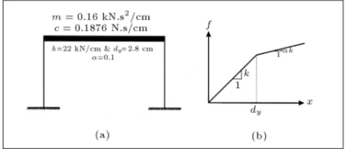
EQUATION OF MOTION OF SDOF FRAMES WITH PRANDTL-ISHLINSKII The equation of motion of a SDOF frame, like the one shown in Figure 2, is comprised of four parts: The inertia, damping and restoring force on the left hand side, and the excitation on the right hand side:
mx + c _x + f(t) = F (t); (7)
where t = time, x = acceleration, _x = velocity, x = displacement, m = mass, c = damping, f(t) = restoring force and F (t) = external excitation. The restoring force in Equation 7 can be rewritten by using the Prandtl-Ishlinskii model, according to Equations 6,
Figure 2. A SDOF frame. (a) Geometry; (b) Bilinear model.
as follows: mx + c _x +
q+1
X
j=1
wj(x zj) = F (t); (8a)
_zj=
(
_x for jx zjj = rj and _x(x zj) > 0
0 otherwise (8b)
where wj and zj are weight and drift of the jth stop
operator. The unknown parameters of Equations 8 are: m, c, wj's and rj's. After the free parameters
of Equations 8 are determined, the response of the frame under any external excitation can be analyzed by solving Equations 8 by an integration scheme, such as the Runge-Kutta method.
IDENTIFICATION METHOD
For any given set of rj values, j = 1; 2; ; q + 1,
Equation 8a can be rewritten in discrete form as follows:
mx(ti) + c _x(ti) + q+1
X
j=1
wj"rj[x(ti)] = F (ti);
i = 1; 2; ::N; (9)
where N is the number of sampling points of the response. Equation 9 can be written in discrete form as:
[A]frg = fBg; (10)
where:
frg = [m; c; w1; ; wq+1]Tr; (11)
fxg = [x1; x2; ; xN]T; (12)
f _xg = [ _x1; _x2; ; _xN]T; (13)
[X] = [Xij];
i = 1; 2; N and j = 1; 2; ; q + 1; (14a)
Xij = "rj[xi]; (14b)
[A] = [fxg; f _xg; [X]]; (15)
fBg = [F1; F2; ; FN]T: (16)
Knowing x, _x, x and F for all the instances i = 1; 2; ; N, the Mean Square Error (MSE) correspond-ing to any vector frg, which is a quadratic function of
frg, is dened as:
MSE (; r) = N1f(er)gfergT; (17)
where:
ferg = fBg [A]frg: (18)
It is now desired to nd the vector frg = frg, where
the value of MSE (; r) is minimum. This is an uncon-strained minimization problem having only one local minimum, which is also the global minimum, because the function, MSE (; r), is quadratic. According to [12], the answer is:
f
rg = ([A]T[A]) 1[A]TfBg: (19)
And the corresponding MSE (; r) is: MSE(r) = 1
Nfe(r)gfe(r)gT; (20a) where:
fe(r)g = fBg [A]f
rg: (20b)
It is noteworthy that the vector of optimum values, f
rg and MSE(r), are unique, because MSE (; r),
which is a quadratic function of frg, has only one
relative minimum, which is also the global minimum. Since the MSE(r) is a function of r, it is now
desired to nd the set of rj values, j = 1; 2; ; q
(noticing rq+1 = 1), for which the MSE(r) is the
minimum. However, in this case, it is not generally possible to assume an analytic form for the MSE(r)
function. There might be dierent algorithms available to solve this unconstraint optimization problem. In this paper, the real Genetic Algorithm (GA), as explained in the next section, has been used, where each chromo-some (string or individual) is identied by an ordered set of genes as follows:
chromosome = [r1; r2; ; rq]; (21)
where:
0 < ri< jxjmax; i = 1; 2; ; q; (22)
and jxjmaxis the maximum of the absolute value of the
displacement. The tness function for a chromosome is dened as:
Fitness = (
M if jri rjj = 0 & i 6= j
MSE(r) otherwise (23)
where M is a large penalty value introduced to avoid the repetition of the same gene values in a chromosome. If the gene values are repeated, then, the matrix, [A]T[A], becomes singular, which in turn does not let
the optimum weights be calculated from Equation 19. The signicant benet of using the GA is that it is a zero-order algorithm, works with the tness values directly and does not depend on its derivatives. A concise explanation of the GA is included in the next section. More details can be obtained from Goldberg [13].
GENETIC ALGORITHM
Genetic Algorithms (GAs) are stochastic optimization techniques, based on the concepts of biological evo-lutionary theory [13,14]. They consist of maintain-ing a population of chromosomes (individuals), which represent potential solutions to the optimization of a function, generally very complex. Each individual in the population has an associated tness, indicating the utility or adaptation of the solution that it represents. A GA starts o with a population of randomly generated chromosomes and advances towards better chromosomes by applying genetic operators, generally modeled on the genetic processes occurring in na-ture. During successive iterations, called generations, the chromosomes are evaluated as possible solutions. Based on these evaluations, a new population is formed using a mechanism of selection through applying the so called genetic operators, including crossover and mutation.
In this paper, a real code GA is utilized. Its outline is described in the following steps:
1. Randomly create an initial population of chromo-somes;
2. Compute the tness of the members of the current population and sort them according to their tness values, with the ttest assigned as the rst; 3. Select parents to mate and produce newborns based
on their tness values. Children are produced either by making random changes to a single parent (mutation) or by combining the genes of a selected pair of parents (crossover);
4. Replace the current population with the children to form the next generation;
5. If the stopping criteria are met, the algorithm will be stopped. Otherwise, go back to step 2.
Three kinds of children are produced in each generation: Elite children, crossover children and mu-tation children. Elite (cloned) children are the best individuals that are cloned from the current population to the next population. The number of elites, (NElite),
crossover, (NCrossover), and mutation, (NMutation),
chil-dren are set in advance and, as a result, the population size will be Npop = NElite+NCrossover+NMutation. The
following genetic operators are used. Roulette-Wheel Selection
Chooses parents by simulating a roulette wheel, in which the area of the wheel is divided into smaller areas representing the individual's expectation of selection. The algorithm uses a random number to select one of the sections with a probability equal to its area. Each
individual's expectation is computed by the following formula:
pi= 1 p
Ri
NPpop
k=1 1 p
Rk
; i = 1; 2; ; Npop; (24)
where pi is ith individual's expectation and Ri is the
rank of the ith individual in the current population, noting that the rank of the best individual is 1. Intermediate Crossover
Creates children by taking a weighted average of the parents. Each child is created from parent1 and parent2 by child = parent1 + rand 0.5 (parent2 - parent1), where rand is a random number in [0,1]. Therefore, for producing NCrossover children,
2NCrossover parents must be selected by the selection
operator.
Uniform Mutation
Uniform mutation is a two-step process. First, the algorithm selects NMutation individuals for mutation,
where each gene has a probability rate of being mu-tated. In the second step, the algorithm replaces each selected gene by a random number, which is uniformly generated in the range dened for that gene.
Stopping Criteria
In this paper, the authors have used a simple stopping criterion. The algorithm stops whenever the generation number reaches a predened maximum number of iterations, denoted by Maxiter.
EXAMPLE 1 A SDOF Frame
It is desired to identify the structural parameters of the SDOF frame shown in Figure 2a. The restor-ing force-displacement relationship follows the bilinear nonlinearity model shown in Figure 2b. In a real test, the frame would be subjected to some known forces, F , and the response would be measured. Hence, the history of response and force, including x, _x, x and F , are recorded. In this study, the experiment has been replaced with numerical simulation, where the frame has been modeled, subjected to dierent excitations and analyzed by the Wilson method of integration. The identication method presented in this paper has then been applied to the results of the numerical simulation and the structure has been identi-ed. The identication results have been compared to
the assumed structural parameters for the assessment of the capability of the identication method.
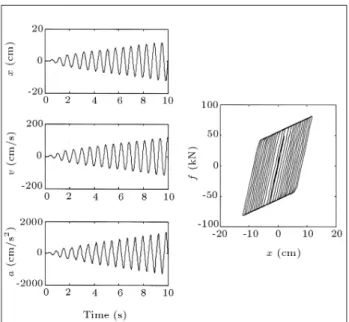
The following excitation has been applied to the frame:
F (t) = 15t sin(10t) kN; (25)
where the corresponding response and hysteresis loop are shown in Figure 3. The acceleration, velocity and displacement signals and the corresponding hysteresis loop are shown in Figure 3. It has been shown that bilinear nonlinearity can be model by Equation 5 with q = 1 [1], therefore, in this example, it is enough to set q = 1. By applying the proposed identication method with NElite = 2, NCrossover = 14, NMutation = 4,
Maxiter = 100 and rate = 0.04, the following
param-eters have been obtained for this frame: r1 = 2:7985
cm, m = 0:1602 kg, c = 0:1878 kN.s/cm, w1= 19:8072
kN/cm, and w2 = 2:2181 kN/cm, where the errors
of identication have been (0.1602-0.16)/0.16=0.12% for m and (0.1878-0.1876)/0.1876= 0.11% for c. The convergence progress of the identication method is depicted in Figure 4, where the convergence has been achieved only in 14 generations. The accuracy of iden-tication of restoring force has been evaluated by using the obtained values for m, c, the Prandtl-Ishlinskii stop parameter, r1, and weights w1 and w2, in the
equation of motion of the SDOF frame (Equations 8), solving the equations by the Runge-Kutta method and, nally, comparing the results with the results obtained from solving the same equations but with the assumed target values for the parameters. Hence, the frame was subjected to 200% of the El Centro earthquake, as shown in Figure 5. The responses are the same for both the identied and target parameters.
Figure 3. Response of the SDOF frame, excited by F (t) = 15t sin(10t) kN.
Figure 4. Convergence characteristics of the GA.
Figure 5. Comparison between target (real) and
identied responses of the SDOF frame excited by 200% El Centro earthquake, where the dierence is not signicant.
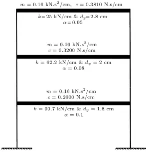
EXAMPLE 2 A MDOF Frame
MDOF shear frames can also be identied by the method proposed in this paper. For example, a three-story shear frame and its parameters are shown in Figure 6. The set of equations of motion of this frame is:
m3x3+ c3_3+ f3= F3(t); (26a)
m2x2+ c2_2+ f2 c3_3 f3= F2(t); (26b)
m1x1+ c1_1+ f1 c2_2 f2= F1(t); (26c)
where f1, f2and f3are the restoring forces of the rst,
Figure 6. Three story frame of Example 2, where structural parameters are dierent for each story.
force, fk, k = 1; 2; 3, can be obtained according to
Equation 5 as follows: fk=
q+1
X
j=1
wk j"rk
j[k]: (27)
Using Equations 27 and 6: fk=
q+1
X
j=1
wk
j(k zkj); (28a)
_zk j =
(
_k for jk zkjj = rjk and _k(k zjk) > 0
0 otherwise (28b)
where k and _k, k = 1; 2; 3 are the interstory
dis-placement and velocity for the kth story, respectively. Equations 26 and 27 are utilized for identication, while Equations 26 and 28 are then used for analyzing the response of the identied frame.
Each of the equations in Equations 26, from (a) to (c), is in fact, the same as the equation of motion (Equation 7) for a SDOF frame. Equation 26a can be solved to nd f3, f3 is substituted in Equation 26b to
nd f2and, then, f2is used with Equation 26c to nd
f1. This method can be generalized by induction for a
shear frame of n stories. Hence, the equation of motion of a shear frame can be summarized as:
mnxn+ cn_n+ fn= Fn(t); (29a)
mkxk+ ck_k+ fk ck+1_k+1 fk+1= Fk(t); (29b)
where k = 1; 2; ; n 1.
The problem is solved for the nth story rst and then proceeds from the top to the bottom of the frame.
In the three-story frame, therefore, the free parameters of the third story are tuned rstly and these parameters are used for identication of the second story and so on. To collect appropriate data for identication, the frame shown in Figure 6 was excited by the following story forces:
F1(t) = 50 sin(7t) kN; (30a)
F2(t) = 75 sin(5t) kN; (30b)
F3(t) = 50 sin(2:5t) kN: (30c)
The response of the frame was then recorded. Similar to the SDOF frame, mass (m), damping (c), r, and two weights, w1and w2, were considered for each of the
oors. The Least Square Error and GA were applied to the MSE and the story parameters were identied for each oor. Table 1 shows the identied parameters of the frame. The identied parameters are very close to the target parameters, which are specied in Figure 6. The displacement of the roof of the identied frame, excited by 200% of the El Centro earthquake, was compared with the real displacement in Figure 7. In this case too, similar to the SDOF frame, their error is not signicant.
CONCLUSIONS
In this paper, the authors have proposed a useful identication method to determine the parameters of
Table 1. Tuned parameters.
k m (kN.s2/cm) c (kN.s/cm) r (cm)
1 0.1599 0.3876 1.7990 2 0.1600 0.3210 1.9994 3 0.1600 0.1996 2.7989
Figure 7. Comparison between the target (real) and identied time history response of the roof displacement of Example 2 under 200% El Centro earthquake.
shear frames with bilinear nonlinearity and the hys-teretic response from the data collected on the forced vibration response of the frames. The method uses Genetic Algorithms (GA) and Quadratic Programming (QP). The main benet of using GA is that it rapidly lets the identication method escape from the local minima and convergence to the nal answer. Through numerical simulations, the method has been applied to both Single Degree Of Freedom (SDOF) and Multi-Degrees of Freedom (MDOF) frames, where the ob-tained identication results have been very accurate. ACKNOWLEDGMENT
The authors would like to thank the Deputy of Higher Education and, also, the Research Deputy of Sharif University, Tehran, Iran for partially supporting this research.
REFERENCES
1. Brokate, M. and Sprekels, J., Hysteresis and Phase Transitions, Springer-Verlag, New York (1996). 2. Iwan, W.D. \A distributed-element model for
hystere-sis and its steady-state dynamic response", J. Appl. Mech., 33(4), pp. 893-900 (1966).
3. Bouc, R. \Forced vibration of mechanical systems with hysteresis", Abstract, Proc., 4th Conference on Nonlinear Oscillation, Prague, Czechoslovakia (1967). 4. Wen, Y.K. \Method for random vibration of hysteretic systems", J. Engrg. Mech. Div., 102(2), pp. 249-263 (1976).
5. Wen, Y.K. \Methods of random vibration for inelastic structures", Appl. Mech. Rev., 42(2), pp. 39-52 (1989). 6. Benedettini, F., Capecchi, D. and Vestroni, F. \Iden-tication of hysteretic oscillators under earthquake loading by nonparametric models", J. Engrg. Mech., ASCE, 121(5), pp. 606-612 (1995).
7. Chassiakos, A.G., Masri, S.F., Smyth, A.W. and Caughey, T.K. \On-line identication of hysteretic systems", J. Appl. Mech., 65(March), pp. 194-203 (1998).
8. Sato, T. and Qi, K. \Adaptive H1 lter: Its
appli-cations to structural identication", J. Engrg. Mech., ASCE, 124(11), pp. 1233-1240 (1998).
9. Smyth, A.W., Masri, S.F., Chassiakos, A.G. and Caughey, T.K. \On-line parametric identication of MDOF nonlinear hysteretic systems", J. Engrg. Mech., ASCE, 125(2), pp. 133-142 (1999).
10. Kosmatopoulos, E.B., Smyth, A.W., Masri, S.F. and Chassiakos, A.G. \Robust adaptive neural estimation of restoring forces in nonlinear structures", J. Appl. Mech., ASME, 68, pp. 880-893 (2001).
11. Visintin, A., Dierential Models of Hysteresis, Springer-Verlag, New York, USA (1994).
12. Nelles, O., Nonlinear Systems Identication from Clas-sical Approaches to Neural Networks and Fuzzy Models, Springer-Verlag, Berlin (2001).
13. Goldberg, D.E., Genetic Algorithm in Search, Op-timization and Machine Learning, Addison-Wesley (1989).
14. Holland, J.H., Adaptation in Natural and Articial Systems, The University of Michigan Press (1975).