Sharif University of Technology
Scientia IranicaTransactions B: Mechanical Engineering www.scientiairanica.com
Research Note
Mathematical modeling and optimization of the
Electro-Discharge Machining (EDM) parameters on
tungsten carbide composite: Combining response
surface methodology and desirability function technique
S. Assarzadeh and M. Ghoreishi
Department of Mechanical Engineering, K.N. Toosi University of Technology, Tehran, P.O. Box 19395-1999, Iran. Received 18 June 2013; received in revised form 29 January 2014; accepted 6 September 2014
KEYWORDS Electro-Discharge Machining (EDM); Response Surface Methodology (RSM); Multi-objective optimization; Desirability Function (DF);
Tungsten carbide cobalt composite (WC-Co); Process modeling.
Abstract. This research proposes a unied scheme to mathematically model and multi-objectively optimize the EDM parameters on tungsten carbide cobalt alloy (WC-6%Co), applying response surface methodology and a desirability function technique. Discharge current, pulse on-time, duty cycle and average discharge voltage have been chosen to be correlated with material removal rate, tool wear rate and surface roughness (Ra) as performance measures. The required experimental data were obtained in accordance with the face-centered central composite design. Signicant parameters in the form of main, two-way interaction and pure quadratic eects were carefully identied conducting a complete analysis of variance at 1%, 5% and 7% signicance levels, and the adequacy of all tted second order regression models was conrmed. Parametric analysis was undertaken through direct and reciprocity eect plots to fully reveal the dierent facets of ED-machinability characteristics. Finally, the optimization issue has been formulated as multi-objective from which the optimal parametric setting, yielding the most enviable conditions simultaneously, was then obtained in a compromised manner employing the notion of a desirability concept. The predicted optimal results were also interpreted and veried experimentally. The values of relative validation errors are all quite satisfactory (below 11%), which prove the ecacy and reliability of the suggested approach.
© 2015 Sharif University of Technology. All rights reserved.
1. Introduction
Electro-Discharge Machining (EDM) is an electro-thermal erosion process, where material is removed by a successive trend of controlled rapid and repetitive dis-crete electrical discharges (sparks), produced by a DC pulse generator, taking place between a pair of tool and work piece electrodes submerged in a liquid dielectric medium [1-3]. For decades, the process has achieved
*. Corresponding author. Tel.: +98 21 84063210; Fax: +98 21 88677274
E-mail address: [email protected] (M. Ghoreishi)
considerably popular applications in machining var-ious engineering materials, especially High-Strength, Temperature-Resistant (HSTR) alloys (Inconel, Tita-nium, Beryllium alloys) [4-6], hard composites (metal matrix composites, nano-composites) [7,8], conductive ceramics [9], etc., and in miscellaneous industries, mostly, aeronautic, die, mould, and automobile in-dustries, with its additional versatility being a very promising approach towards micro- as well as nano-machining technologies [10].
The literature reveals that a large amount of research work has mainly been focused on studying the EDM characteristics in dierent types of steel,
using either dierent combinations of tool materials or process modication, with some conventional routines, known as hybrid machining techniques, to enhance process productivity and accuracy [1,2,11]. In this context, researchers have mainly applied statistically designed or soft-computing-based techniques to model and optimize process parameters and responses. How-ever, unlike steel often chosen as a general option for work piece material in EDM applications, it has been postulated that the behavior of ceramic compos-ites, such as tungsten carbide-cobalt composite, can be rather dierent in response to various parameters under the EDM process [9]. Tungsten carbide-cobalt composite, amongst the most widely used dicult-to-cut materials, is one of the most important engi-neering materials with extreme applications commonly employed in manufacturing carbide dies and molds, cutting tools, forestry tools, and components resisting continual wear in production lines. Its acutely high hardness and strength, superior wear and corrosion resistance over a wide range of temperatures has frustrated conventional machining processes in being utilized eciently in shaping such a material. Although the EDM process has now been recognized and justied as the best and perhaps the only procient machining candidate for cutting and shaping tungsten carbides, the process is not an easy going task [3,12]. The main diculty in EDMing WC-Co originates from its non-homogeneous structure, the dierences between the melting and evaporation points of the two constituent phases present in its micro-structure, i.e. WC and Co grains, which may cause non-uniformity in erosion as well as process instability, producing short circuits and arcing pulses more frequently [12]. The melting and vaporization points of WC are about 2800C
and 6000C, respectively, and those for Co are about
1320C and 2700C, both at normal atmospheric
pres-sure [13,14]. Hence, during the EDM, the cobalt matrix rst starts being removed from the surface by melting and evaporation mechanisms due to sparking. This early selective decomposition of the WC-Co structure will lead to dislodging coarse WC grains into the gap space, increasing the risk of process instability as a result of high debris accumulation and pollution inside the gap region. Moreover, there is a noticeable dierence in the thermal expansion coecient of WC and Co, the latter possessing a much higher one (14 10 61=C for Co as compared to 5 10 61=C
for WC) [14]. The discrepancy is responsible for developing high thermal tension stresses during re-solidication and quenching, exceeding the fracture strength of the material in the crater, and thus, causing an abundance of cracks on the surface layer. For these reasons, the electro discharge machining of WC-Co composite is regarded as a challenging task imposing more diculties compared to EDMing dierent kinds
of hardened steels commonly studied in research arti-cles.
1.1. Literature review
Lee and Li [15] studied the eects of EDM parameters on the surface characteristics of a kind of tungsten carbide. They concluded that the MRR and surface roughness of the work piece are directly proportional to the discharge current intensity. In further research [16], they undertook a comprehensive qualitative analysis of the surface integrity of ISO standard P -grade tungsten carbide under EDM conditions with peak current and pulse on-time variations. Miscellaneous aspects of surface integrity, like micro-cracks, recast layer for-mation and surface roughness, were studied. It was pointed out that the quality of the work surface is a function of two main parameters, peak current and pulse duration, both of which are settings of the power supply. In a more quantitative manner, Puertas et al. [17] applied a 23 full factorial design with four
center points to provide protection against curvature in the model building of EDMing 94WC-6Co ceramic composite solely under nishing stages. Although dif-ferent signicant main and interaction eects between input parameters were identied using ANOVA, and their variations over selected responses were studied, neither denite input settings nor a numerical value of machining factors were obtained as optimum values, since no suitable optimization strategy was then tried. Once more, the same previous authors [18] conducted a comparative study of the die sinking EDM of three dierent conductive ceramics, viz. WC-Co, B4C, and
SiSiC in terms of MRR, Ra, and TWR as response technological variables, using the same aforementioned DOE plan under only a nishing regime, using low discharge energy levels. They indicated that the inves-tigated ceramic materials showed dierent behaviors in response to the alterations of input factors, except for the MRR function, which manifested the same trend for all the work piece materials. In another study, Lin et al. [19] investigated the eects of electrical discharge energy on the machining characteristics of two kinds of cemented tungsten carbide, grades K10 and P 10. They pointed out that there exists a particular range of machining parameters within which the process is stable, and exceedingly long or short pulse duration causes instability. As a soft computing based opti-mization strategy, Kanagarajan et al. [20] employed non-dominated sorting genetic algorithm (NSGA-II) to obtain a Pareto optimal series of input variables in a tradeo manner. However, neither the role of pulse o-time as an independent variable nor the inclusion of tool wear phenomenon as an important response was taken into account, as both can denitely aect the process productivity, cost, and dimensional accuracy of machined parts. Once more, Kanagarajan et al. [21]
applied RSM, along with multiple linear regression analysis, to obtain second order response equations for MRR and Ra in EDMing WC/30%Co composite. Though the most inuential parameters aiming at maximizing MRR and minimizing Ra were identied by carefully examining the surface and contour plots of the responses, again, their suggested approach suers from the same aforementioned drawbacks. Banerjee et al. [22] applied a Face-Centered Central (FCC) composite design to collect experimental data and RSM to model and analyze the processing parameters involved in EDMing WC-TiC-TaC/NbC-Co cemented carbide. They found that sucient superheating of work piece material and subsurface boiling are essential for ecient material removal, and that the formation of pock marks due to the bursting of blisters and associ-ated crack formations may be controlled by choosing a proper combination of dielectric and interfering inuen-tial parameters. Finally and most recently, Puertas and Luis [23] studied the behavior of two highly practical conductive ceramics in industry, B4C and WC-Co
under dierent die sinking EDM conditions. Though practical recommendations on how to adjust process settings to acquire low surface roughness, low electrode wear, and high MRR were suggested independently, neither a precise optimization strategy nor a denite numerical parametric setting was then proposed to tradeo between those conicting objective responses, as they were treated autonomously from each other without considering their mutual interdependencies. 1.2. Structure and contributions of the current
research
Based on the previously stated information in opening the basic subject and reviewing related past research, the major motivation of the present study is to fully understand and characterize the machinability mea-sures of WC-6%Co in a more quantitatively systematic way in order to identify the correct eects of various interfering parameters inuencing process responses. In this regard, the face-centered Central Composite Design (CCD) of experiments has been adopted to plan the experiments. Adequately sucient second order response equations, i.e. MRR, TWR, and Ra, are de-veloped based on RSM, using multiple linear regression analysis, along with ANOVA, in which both signicant main and two-factor interactive eects are presently pre-documented by student t-tests. Subsequently, the mathematical forms of process responses are optimized to yield the best operating parameter combinations, satisfying the highest possible MRR, lowest TWR and Ra, simultaneously, in a compromised manner, using an aggregated desirability function idea. The foremost merits of the current research can be mentioned as follows:
a) By far, to the best of the authors' knowledge
acquired through extensive review of related lit-erature, the simultaneous numerical optimization of MRR, Ra, and TWR in the EDM of tungsten carbide has not yet been implemented. In the bibliography consulted, there is still a lack of practical knowledge on EDMing WC-Co, as few technological tables useful for both EDM practi-tioners and academicians can be found compared to those widely available for miscellaneous kinds of hardened steel.
b) Despite the fact that several experimental works have been directed towards studying EDMing WC-Co from dierent aspects [12], in their best cases, they have either ended at the point of merely developing respective responses without any at-tempt to highlight exact numerical optimal condi-tions [19], or obtaining optimal condicondi-tions without bearing in mind the possible interdependencies of all three main outputs (MRR, TWR, and Ra) at the same time, as one of which has often been neglected [20,21,23]. In addition, no eort has yet been put into applying the desirability function method, aiming to optimize the EDM parameters of WC-6%Co composite.
2. Experimental details
2.1. Machine tool, tool electrode, work piece and dielectric materials
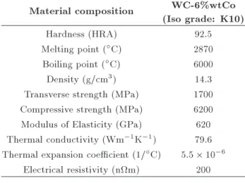
An Azarakhsh ZNC spark erosion machine, model number 204, has been used to run the experiments. Equipped with an iso-frequency pulse generator, it can produce pulse-on times in the range 2s-1000s and provide maximum discharge current up to 75 A. Tungsten carbide cobalt composite, type WMG10, manufactured by the Wolframcarb Company, Italy, available in cylindrical form with 12 mm diameter, has been selected as the work piece material for all tests. The selected WC-Co composite, produced via powder metallurgy, having about 94%wt WC and 6%wt Co as its nominal chemical composition, is of a ne grain type and mainly used in fabricating drawing dies and woodworking tools, as well as cutting tools for non-ferrous metals. Table 1 lists the relevant work piece material properties.
Electrolytic copper rods with the same diameter as the work piece were used for the tool electrode material. The physical and mechanical properties are a density of 8.9 g/cm3, thermal conductivity 226 W/mK,
electrical resistivity 9 cm, melting point 1083C, and
hardness of about 100 HB. Copper has the additional advantage of being easily available, stable in quality and cheap compared to other applicable metals. The EDM experiments were all conducted in a planing mode in which both the tool and work piece bottom
Table 1. Work piece thermo-physical and mechanical properties.
Material composition WC-6%wtCo (Iso grade: K10)
Hardness (HRA) 92.5
Melting point (C) 2870
Boiling point (C) 6000
Density (g/cm3) 14.3
Transverse strength (MPa) 1700 Compressive strength (MPa) 6200 Modulus of Elasticity (GPa) 620 Thermal conductivity (Wm 1K 1) 79.6
Thermal expansion coecient (1/C) 5:5 10 6
Electrical resistivity (nm) 200
Figure 1. (a) Picture of Azarakhsh ZNC 204 EDM machine, and (b) work/tool electrode samples.
surfaces were ground, prior to experimentation, to remove any possible machining marks or irregularities, and assuring consistent initial gap width and ushing action. Moreover, commercial grade kerosene ejected as impulse side ushing through a nozzle was used as the dielectric liquid carrying out machining debris from the gap zone. Also, the tool and work piece electrode polarity were assigned as positive and negative, respec-tively, as this status can make tool wear minimum, along with having stable sparking [9]. Figure 1(a) and (b) show a photograph of the EDM machine and work piece/tool samples used in experiments.
2.2. Machining parameters, design of experiments, and measurements
Four controllable input variables, namely, discharge current (A: Amp), pulse-on time (B: s), duty cycle (C: %), and average gap (reference) voltage (D: Volt) have been selected as predominant factors, based on the EDM machine operating characteristics and by con-sulting the respective bibliography [1,2], being the most eective parameters governing discharge energy, which directly aects process performance and eciency.
The face-centered central composite design [24-26], a popular variant of the Central Composite Design (CCD) of experiments, has been employed to plan the experiments. It is a kind of second order design class, which uses three levels for each parameter and can eciently handle linear, quadratic, as well as interaction terms, in process modeling. Generally, to collect enough data to establish a suitable second order regression response equation for a process involving k variables, the following three sets of design points are needed:
(a) nf = 2k factorial design or corner points;
(b) na = 2k axial or star points; and
(c) nc center points, which are usually repeated
sev-eral times to obtain a good estimation of experi-mental pure error.
The factorial points contribute in a major way to the estimation of linear and two-factor interaction terms, while axial points contribute in a large way to the estimation of quadratic terms. The center runs will also provide an internal estimate of error (pure error) and contribute to the prediction of quadratic terms [24-26].
To obtain a proper second order response surface equation, these are the minimum as well as optimum number of experimental runs. Though other ap-proaches, such as the Taguchi design technique, which may need a smaller number of trails, can be applied, it suers from serious drawbacks, the most important of which is its inability to obtain all the possible interaction eects [24-26]. Identifying and obtaining all interaction terms can be of vital importance in process modeling and optimization, and CCD assures such a trend [24-26].
Therefore, the total number of experiments would be:
N = nf+ na+ nc= 2k+ 2k + nc: (1)
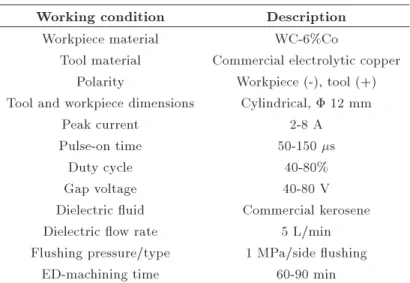
The location of axial points in a response surface central composite design, with respect to the center point (origin), is determined by alpha () value. The choice of depends, to a great extent, on the domain of operation and interest [25]. In face-centered central composite design, = 1, meaning a three-level design space, coded as -1, 0, and 1, corresponds to low, medium, and high parameter levels, respectively. To specify the actual levels of each input variable, at rst, a number of preliminary tests were conducted as a One-Factor-At-a-Time (OFAT) approach to determine the most stable combination of parameter settings over the operability region of the EDM machine [27]. Table 2 summarizes the relevant machining conditions and xed parameters, whereas Table 3 lists the preferred
Table 2. The EDM conditions.
Working condition Description
Workpiece material WC-6%Co
Tool material Commercial electrolytic copper Polarity Workpiece (-), tool (+) Tool and workpiece dimensions Cylindrical, 12 mm
Peak current 2-8 A
Pulse-on time 50-150 s
Duty cycle 40-80%
Gap voltage 40-80 V
Dielectric uid Commercial kerosene
Dielectric ow rate 5 L/min
Flushing pressure/type 1 MPa/side ushing
ED-machining time 60-90 min
Table 3. Independent input factors and levels for the face-centered CCD. Parameter Notation Unit Coded/Actual level
-1 0 +1
Discharge current (I) A Ampere 2 5 8
Pulse on-time (Ton) B s 50 100 150
Duty Cycle (DC) C - 40 60 80
Gap voltage (V) D Volt 40 60 80
input controllable parameters, along with their ranges in both coded and actual format.
The response variables were then chosen as ma-terial removal rate (MRR: g/h), tool wear rate (TWR: g/h), and average surface roughness (Ra: m). Both the stock removal rate and tool wear rate were mea-sured directly by the weight loss method, weighing the work piece and tool electrode samples before and after each test and dividing the corresponding weight dierence by the elapsed time allocated for each experimental run. A GX-200 digital single pan balance, manufactured by the A&D Company, Japan, with a precision of 0.001 g and maximum capacity of 210 g, has been used for the evaluation. During the running of the rst round of experiments, it was revealed that much longer times were needed to get a reasonable idea about the MRR [27]. So, the time allocated to each trial was at least an hour, and much longer times were considered for runs with lower discharge currents. Characterization of each work piece surface condition was conducted in terms of arithmetic mean deviations of the roughness prole from the central line along the measurement path. A Mahr-PS1 unit, a portable stylus type prolometer made-up by the Mahr Company, Germany, was used for roughness assessments. Before measuring surface roughness, each machined sample was cleaned in acetone liquid and dried with a cold air blower. To achieve validity and accuracy, each Ra
measurement was repeated twice along two dierent directions, as there is no specic pattern for spark distribution over the work area. The average of the two replications was then assigned as the roughness value for each treatment combination. In all cases, a cuto length of 0.8 mm and an evaluation length of 4 mm (5 0:8 mm) were adjusted on the unit, according to ISO 4287/1.
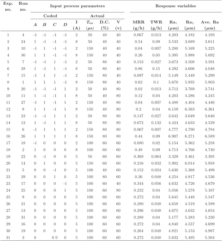
By repeating seven center points, the total num-ber of conducted experiments for k = 4 was 24+2(4)+
7 = 31, and are shown in Table 4, along with the cor-responding process responses. The linear relationship between coded and actual values, in Tables 3 and 4, is as follows:
Discharge current:
A = [I (Imax+ Imin)=2] =(Imax Imin)=2:
Pulse on-time:
B=[Ton (Tonmax+Tonmin)=2] =(Tonmax Tonmin)=2:
Duty cycle:
C=[DC (DCmax+DCmin)=2] =(DCmax DCmin)=2:
Gap voltage:
Table 4. Design layout and experimental results. Exp.
no.
Run
no. Input process parameters Response variables
Coded Actual
A B C D I
(A) Ton
(s)
D.C. (%)
V (v)
MRR (g/h)
TWR (g/h)
Ra1
(m) Ra2
(m)
Ave. Ra (m)
1 4 -1 -1 -1 -1 2 50 40 40 0.067 0.013 4.203 4.182 4.193
2 24 1 -1 -1 -1 8 50 40 40 0.54 0.09 3.533 3.689 3.611
3 10 -1 1 -1 -1 2 150 40 40 0.04 0.007 5.280 5.169 5.225
4 30 1 1 -1 -1 8 150 40 40 0.26 0.05 5.395 5.988 5.692
5 7 -1 -1 1 -1 2 50 80 40 0.153 0.027 3.673 3.508 3.591
6 28 1 -1 1 -1 8 50 80 40 0.86 0.15 4.292 4.606 4.048
7 15 -1 1 1 -1 2 150 80 40 0.097 0.014 5.149 5.449 5.299
8 1 1 1 1 -1 8 150 80 40 0.62 0.1 5.670 5.935 5.803
9 20 -1 -1 -1 1 2 50 40 80 0.02 0.013 3.712 3.769 3.741
10 11 1 -1 -1 1 8 50 40 80 0.12 0.04 4.203 4.286 4.245
11 27 -1 1 -1 1 2 150 40 80 0.04 0.007 4.488 4.404 4.446
12 8 1 1 -1 1 8 150 40 80 0.2 0.04 6.159 6.563 6.361
13 23 -1 -1 1 1 2 50 80 80 0.147 0.027 3.642 3.649 3.646
14 12 1 -1 1 1 8 50 80 80 0.672 0.132 4.424 4.633 4.529
15 6 -1 1 1 1 2 150 80 80 0.067 0.007 4.777 4.790 4.784
16 26 1 1 1 1 8 150 80 80 0.44 0.09 6.907 6.271 6.589
17 18 -1 0 0 0 2 100 60 60 0.080 0.02 5.154 5.362 5.258
18 2 1 0 0 0 8 100 60 60 0.48 0.09 4.713 4.766 4.740
19 22 0 -1 0 0 5 50 60 60 0.368 0.064 3.329 3.461 3.395
20 14 0 1 0 0 5 150 60 60 0.216 0.032 5.902 6.014 5.958
21 5 0 0 -1 0 5 100 40 60 0.152 0.024 5.630 5.368 5.499
22 29 0 0 1 0 5 100 80 60 0.36 0.048 4.254 4.817 4.536
23 17 0 0 0 -1 5 100 60 40 0.344 0.056 4.632 4.726 4.679
24 25 0 0 0 1 5 100 60 80 0.232 0.04 5.056 5.278 5.167
25 9 0 0 0 0 5 100 60 60 0.272 0.04 5.645 5.448 5.547
26 21 0 0 0 0 5 100 60 60 0.280 0.048 4.658 4.519 4.589
27 13 0 0 0 0 5 100 60 60 0.296 0.048 4.675 4.632 4.654
28 31 0 0 0 0 5 100 60 60 0.288 0.04 5.177 5.283 5.230
29 16 0 0 0 0 5 100 60 60 0.272 0.04 4.840 4.557 4.699
30 19 0 0 0 0 5 100 60 60 0.264 0.048 4.821 5.153 4.987
31 3 0 0 0 0 5 100 60 60 0.272 0.048 5.632 5.495 5.564
where A, B, C and D are the coded values of variables I, Ton, DC, and V , respectively, Imax, Tonmax, DCmax,
and Vmaxrepresent the maximum values of I, Ton, DC,
and V , respectively, and, Imin, Tonmin, DCmin, and
Vminare the corresponding minimum values of process
parameters in each interval. Finally, it is to be noted that the order of experimentation was randomized, according to the second column of Table 4, to avoid the creeping eect of any possible extraneous or nuisance factors into the results [24].
3. Response surface modeling of process outputs
The practical optimization of EDM parameters on WC-Co composite necessitates the accurate model build-ing of the process responses describbuild-ing its behavior and characteristics under dierent operating condi-tions. Response Surface Methodology (RSM) [24-26], a collection of mathematical and statistical techniques aimed at developing suitable second order polynomial
models, relating a number of input variables to selected responses by multiple linear regression analysis, has been employed here. The model, in terms of the observations, in matrix notation, is:
y = X + "; (2) where y is a (n 1) vector of observations (n is the number of observations), X is an (n p) matrix of the levels of the independent variables (p = k + 1, k is the number of process variables or regressors), is a (p 1) vector of the regression coecients and " is an (n 1) vector of random errors. The vector of tted values, ^yi, corresponding to the observed values,
yi (tted regression model), is then [25]:
^y = X ^; (3)
where ^ is the least squares estimator of regression co-ecients () [0; 1; 2; :::; k]T, and can be calculated
based on the following equation: ^
= (X0X) 1X0y: (4)
In the above equation, X0 is the transpose of matrix
X, X0X is a (p p) symmetric matrix, and X0y is a
(p 1) column vector. Therefore:
^y = X ^ = X(X0X) 1X0y = Hy: (5)
The n n matrix H = X(X0X) 1X0 is usually called
the hat matrix, which plays a central role in regression analysis and in mapping the vector of observed values into a vector of tted values. The dierence between the actual observed value, yi and the corresponding
tted value, ^yi, is the residual, ei = yi y^i, a (n 1)
vector. The n residuals may be conveniently written in matrix notation as:
e = y ^y = y X ^ = y Hy = (I H)y; (6) where I is an (nn) identity matrix. In scalar notation, the general form of a tted response surface quadratic model can be written as:
^y = 0+ k
X
i=1
ixi+ k
X
i=1
iix2i + k 1
X
i=1 k
X
j=i+1
ijxixj:
(7) The intercept coecient, 0, represents the response at
the center of the experiments, where all the variables are zero (in coded form); i, ii, and ij also show
the linear, quadratic, and linear-by-linear interaction eects of the parameters, respectively. This second-order polynomial is the most commonly used form and works quite well for a relatively small region of the variable space. By applying the Least Squares Method (LSM) [24-26], all these coecients in a multiple regression model can be estimated.
In this study, the quantitative form of the rela-tionship between desired responses and independent input variables can be represented by the following form:
y = f(I; Ton; DC; V ); (8)
where y is the desired response and f is the response function or surface. The steps consisting of applying regression analysis, performing pooled ANOVA on each obtained regression coecients to nd statistically signicant terms, and nally, conducting ANOVA and some routine statistics to check modeling adequacy and goodness of t, are the necessary actions needed to be carefully executed to nd the suitable reduced quadratic forms of response functions, MRR, TWR, and Ra for the highly stochastic process of EDM. The next sections focus on these procedures.
3.1. Mathematical modeling of MRR, TWR, and Ra
Based on the model described by Eq. (8) and by apply-ing the LSM, all the regression coecients pertainapply-ing to the three responses have been obtained and are shown in Table 5, along with their corresponding Student T - and P -values as a pooled ANOVA format. As is clear from this table, all the main eects of four input parameters (A: discharge current, B: pulse on-time, C: duty cycle, and D: gap voltage) are found to be highly signicant, at least at a = 0:01 signicance level or 99% condence interval, having almost zero P -values, in aecting both the MRR and TWR. However, for the third response, Ra, just the rst two factors, discharge current (A) and pulse-on time (B) are regarded as the highly signicant main factors. In the terminology of statistical modeling, the lower the P -value, the more inuential is the eect [24-26]. On the other hand, the pure quadratic eect of duty cycle (C2), the
two-way interactions of discharge current with pulse-on time (A B), with duty cycle (A C), and with gap voltage (A D), as well as the interaction amongst the pulse on-time with duty cycle (B C), were also found to be extremely important terms inuencing MRR. For the TWR measure, the dual interactive eects amid current with pulse-on time (A B), with duty cycle (A C), and with gap voltage (A D), plus pulse on-time and duty cycle (B C), along with the second order eects of discharge current (A2) and
duty cycle (C2), were made known to have inuencing
outcomes. Finally, for the Ra quality measure, the only considerable interactive terms are the discharge current with pulse-on time (A B) and with gap voltage (A D). As a whole, the inclusion of any term with a P -value less than 0.07 designated as an upper bound for statistical signicance, i.e. being signicant within 93% of condence interval, has been guaranteed in this research, so as to increase each model's accuracy
Table 5. Regression coecients and T -test results for the individual MRR, TWR and Ra model parameters.
Predictor MRR model TWR model Ra model
Coecient T -value P -value Coecient T -value P -value Coecient T -value P -value Constant 0.2790 80.939 0.0001a 0.0449 22.803 0.0001a 5.0082 38.649 0.0001a
A 0.2003 34.796 0.0001a 0.0359 22.957 0.0001a 0.3019 2.933 0.010a
B -0.0631 -17.705 0.0001a -0.0116 -7.416 0.0001a 0.8421 8.179 0.0001a
C 0.1029 17.869 0.0001a 0.01728 11.035 0.0001a -0.0104 -0.101 0.920
D -0.0527 -14.787 0.0001a -0.0062 -3.939 0.001a 0.0759 0.738 0.471
A2 -0.0004 -0.058 0.954 0.0096 2.337 0.033b 0.0263 0.097 0.924
B2 0.0116 1.602 0.137 0.0026 0.640 0.531 -0.2962 -1.092 0.291
C2 -0.0244 -3.379 0.006a -0.0094 -2.270 0.037b 0.0448 0.165 0.871
D2 0.0076 1.048 0.317 0.0026 0.640 0.531 -0.0497 -0.183 0.857
AB -0.0375 -7.249 0.0001a -0.0054 -3.274 0.005a 0.2143 1.962 0.067c
AC 0.0718 10.074 0.0001a 0.0136 8.167 0.0001a 0.0841 0.770 0.453
AD -0.0481 -9.306 0.0001a -0.0051 -3.048 0.008a 0.2663 2.439 0.027b
BC -0.0207 -4.002 0.002a -0.0046 -2.747 0.014b 0.0454 0.416 0.683
BD 0.0067 1.687 0.120 0.0026 1.543 0.142 -0.0348 -0.319 0.754
CD 0.0080 1.539 0.152 0.0016 0.941 0.361 0.0459 0.421 0.680
a: Signicant at = 1% signicance level;b: Signicant at = 5% signicance level;c: Signicant at = 7% signicance level.
and adequacy as highly as possible. All the other terms not meeting such a criterion are supposed to be insignicant. Generally, the term \interaction" means that the eect of a factor over a known response depends on the level of another factor. Identifying signicant interaction terms in the RSM model building procedure and their inclusions in the structure of a second order model are of vital importance, as they can reveal very crucial phenomena of the combinatorial joint eects of dierent process parameters on every process characteristic and behavior [24-26].
Removing insignicant terms is a common prac-tice amongst empirical model builders which, in most cases, can result in improved model tting capabilities, aside from yielding a simpler model form. Thus, the insignicant terms have been excluded from the model structures through a backward elimination method [24-26], and the ANOVA has been repeated for every obtained reduced quadratic model containing only those signicant terms contributing to model building. Table 6 illustrates the ANOVA results for the three response functions. As desired, all the quadratic regression models are signicant, while their lacks of ts turned out to be insignicant relative to pure error. Hence, the model adequacy checking is completely assured for each output measure. Other statistical diagnostic indices mainly used to evaluate the mod-eling goodness of t are the ordinary R-squared (R2),
adjusted R-squared (R2
Adj), and predicted R-squared
(R2
Pred) [26], shown in Table 6, for every response
model. The values are 99.74%, 99.59%, and 98.51% for MRR; 97.58%, 96.38%, and 91.13% for TWR; and
80.93%, 77.12%, and 74.1% for Ra, respectively. As a general rule, the more the R2s approach unity, the
better the model ts the experimental data [24-26]. The usual statistic, R2, also called the coecient of
multiple determination, indicates how many percent of the total variations can be explained by the model, while the R2
Adj, a statistic adjusted for the size (the
number of factors) of the model, means how many percent of the total variability can be explained by the model after considering the signicant terms (re-duced model). The amount of R2 increases as each
additional variable or regressor, whether signicant or insignicant, is added to the model. On the contrary, the adjusted R2does not automatically increase when
new predictor variables are added to the model. In fact, the value of adjusted R2 will often decrease when
unnecessary terms are included. Accordingly, when R2
and R2
Adj dier dramatically, there is a good chance
that non-signicant terms have been incorporated in the model [24-26]. Therefore, it is a suitable criterion in evaluating a model's goodness of t when only signicant terms are involved, compared to the case when all the terms are caught up. The statistic PRESS (prediction error sum of squares) is a measure of how well the model will predict new data. A model with a small value of PRESS is desired, as it indicates that the model is likely to be a good predictor [25]. In connection with this, the predicted R2 (R2
Pred)
is dened, which is an indication of the predictive capability of the regression model in response to new observations.
Table 6. ANOVA table for the trimmed MRR, TWR and Ra second order models.
Source DF Seq SS Adj MS F value P value Remarks
(a) For MRR
Regression 9 1.05761 0.11751 676.09 0.000 Signicant
Linear 4 0.98063 0.22721 1307.20 0.000
Square 1 0.00825 0.00066 3.79 0.069
Interaction 4 0.06874 0.01718 98.86 0.000
Residual error 16 0.00278 0.00017 -
-Lack-of-t 10 0.00250 0.00021 1.68 0.271 Insignicant
Pure error 6 0.00073 0.00012 -
-Correlation total 25 1.06039 - -
-R2= 99:74% R2
Adj= 99:59% R2Pred= 98:51% PRESS = 0:01577
(b) For TWR
Regression 10 0.03641 0.00364 8 0.76 0.000 Signicant
Linear 4 0.03174 0.00794 176.02 0.000
Square 2 0.00051 0.00025 5.64 0.011
Interaction 4 0.00415 0.00104 23.07 0.000
Residual error 20 0.00090 0.00005 -
-Lack-of-t 14 0.00079 0.00006 3.09 0.086 Insignicant
Pure error 6 0.00011 0.00002 -
-Correlation total 30 0.03731 - - -
-R2= 97:58% R2
Adj= 96:38% R2Pred= 91:13% PRESS = 0:00331
(c) For Ra
Regression 5 16.379 3.2758 21.22 0.000 Signicant
Linear 3 14.510 4.8365 31.33 0.000
Interaction 2 1.870 0.9348 6.06 0.007
Residual error 25 3.859 0.1544 -
-Lack-of-t 9 1.942 0.2158 1.80 0.146 Insignicant
Pure error 16 1.917 0.1198 -
-Correlation total 30 20.239 - -
-R2= 80:93% R2
Adj= 77:12% R2Pred= 74:10% PRESS = 5:24248
calculated as [25]: R2= SSR
SST = 1
SSRes
SST ; (9)
R2
Adj= 1 SSSSRes=(n p) T=(n 1) = 1
MSRes
MST
= 1
n 1 n p
(1 R2); (10)
R2
Pred= 1 PRESSSS
T ; (11)
PRESS =Xn
i=1
e2 (i)=
n
X
i=1
yi ^y(i)2; (12)
where SSR is the regression sum of squares, SST is
the total sum of squares, SSRes is the residual sum of
squares, MSRes is the residual mean square, MST is
the total mean square, and ^y(i) is the predicted value
of the ith observed response based on a model t to the remaining (n 1) sample points.
A broad overview of these indices conrms the suitability and completeness of all the obtained mod-els, as neither inconsistency nor poor adequacy can be observed. A complete residual analysis has also been undertaken for every developed response and the graphs are shown in Figure 2(a)-(c). A normal probability plot of residuals reveals that experimental data are spread approximately along a straight line, conrming a good correlation between experimental and predicted values for the response (Figure 2, a(A), b(A), and c(A)). In the graph of residuals versus tted values (Figure 2, a(B), b(B), and c(B)), only small variations can be seen. The histogram of residuals (Figure 2, a(C), b(C), and c(C)) also shows a Gaussian
Figure 2. Plot of residuals: (a) MRR; (b) TWR; and (c) Ra. (A) normal probability plot of residuals; (B) residuals versus the tted values; (C) histogram of the residuals; and (D) residuals against the order of data.
distribution, which is desirable. Finally, in residuals against the order of experimentations in Figure 2, a(D), b(D), and c(D), both negative and positive residuals are apparent, indicating no special trend, which is worthy from a statistical point of view. As a whole, all the yielded models show no inadequacy.
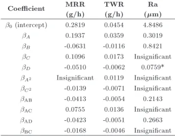
Table 7 details all the numerical values of nalized individual regression coecients for every response. Based on these, the mathematical equations are con-formed for each performance characteristics to be suitable coecients and can be expressed in terms of coded factors as:
MRR =0:282 + 0:194A 0:063B + 0:11C 0:051D 0:014C2 0:041A B + 0:076A C
0:042A D 0:017B C; (13)
TWR =0:045 + 0:036A 0:012B + 0:017C 0:006D + 0:012A2 0:007C2
0:005A B + 0:014A C 0:005A D 0:005B C; (14) Ra =4:849 + 0:302A + 0:842B + 0:076D
+ 0:214A B + 0:266A D: (15) The above developed models can be used as reliable tools navigating the design space within the process parameters domain to get an in-depth understanding of process characteristics, and can also be utilized in the optimization stage to nd optimum EDMing conditions on WC-6%Co.
Table 7. Finalized regression coecients of the response models.
Coecient MRR
(g/h)
TWR (g/h)
Ra (m) 0 (intercept) 0.2819 0.0454 4.8486
A 0.1937 0.0359 0.3019
B -0.0631 -0.0116 0.8421
C 0.1096 0.0173 Insignicant
D -0.0510 -0.0062 0.0759*
A2 Insignicant 0.0119 Insignicant C2 -0.0139 -0.0071 Insignicant AB -0.0413 -0.0054 0.2143
AC 0.0755 0.0136 Insignicant
AD -0.0423 -0.0051 0.2663
BC -0.0168 -0.0046 Insignicant The eect of gap voltage (D) on surface
roughness is insignicant (see Table 5) and its coecient has just been kept to comply with the hierarchy principle.
The EDM is an inherently stochastic and complex process, and it would be of interest to check the variability of output responses, i.e., MRR, TWR, and Ra, when an experiment is repeated using the same set of input parameter settings. It is also of great importance to test the generalization capabilities of de-veloped models in response to some input data settings not used in the DOE plan but lying within the limits of input parameter domains. These investigations can helpfully provide fair justice to how robust the response surface models are in points of the reliability of gathered data used for model building, as well as models' predictive capabilities. Table 8 lists a set of ve repetitive experimental runs selected randomly from Table 4, which account for checking the variability of output responses, while Table 9 presents a set of ve additional tests, carefully designed to be dierent from those used for model building, to check the predictive accuracy of the developed models.
It is to be noted that the number shown in parenthesis in the rst column of Table 8 corresponds to the experimental number in Table 4, for which the experimental setting has been repeated.
It can be inferred from Table 8 that there exists an acceptable level of variability when some experiments are repeated. The amounts of each two repetitive output responses are in close proximity to each other, assuring that the data base obtained from the adopted FCC design could reliably represent the EDM behavior of WC/6%Co under dierent conditions and could condently be used for model development The average percentage deviations are 1.84%, 0.42%, and 15.3% for MRR, TWR, and Ra over these ve repetitions, respectively. The values are obviously acceptable in view of engineering applications.
Table 9 illustrates the results of several conr-mation experiments conducted to check the accuracy of each response model. The values of mean relative prediction errors are 8.75%, 10.30%, and 4.96% for MRR, TWR, and Ra, respectively. Therefore, it can be concluded that the obtained second-order response equations are quite adequate, possessing reasonable accuracy, to capture the highly nonlinear trends of EDM measures, and can satisfactorily be used for further analysis and optimization purposes.
4. Results and discussion
To genuinely describe the quality of variation trends of each process response with respect to inputs, it is of great importance to be aware that spark energy is the dominant factor most responsible for the mechanism of material removal in EDM. The amount of discharge energy (q) delivered per single discharge, assuming a normal pulse (i.e. spark), can be expressed as [28]:
q = Z Ton
Td
VdisIdisdtVdis:Idis:(Ton Td)Vdis:Idis:Ton;
(16)
Table 8. Experimental checking of the repeatability of output response data. Exp.
no
Input process
parameters Response variables
Percentage variation
(%) I
(A) Ton
(s) DC (%)
V (v)
MRR1
(g/h)
MRR2
(g/h)
TWR1
(g/h)
TWR2
(g/h) Ra1
(m) Ra2
(m) MRR TWR Ra
1 (4) 8 150 40 40 0.260 0.230 0.050 0.057 5.692 5.511 3 0.7 18.1
2 (9) 2 50 40 80 0.020 0.023 0.013 0.011 3.741 3.904 0.3 0.2 16.3
3 (17) 2 100 60 60 0.080 0.073 0.020 0.023 5.258 5.424 0.7 0.3 16.6 4 (20) 5 150 60 60 0.216 0.244 0.032 0.036 5.958 5.837 2.8 0.4 12.1 5 (24) 5 100 60 80 0.232 0.256 0.040 0.035 5.167 5.301 2.4 0.5 13.4
Mean percentage variation (%) 1.84 0.42 15.3
Percentage variation (%) = jR1 R2j 100, where R1and R2 stand for the rst and second repetition of each response,
Table 9. Experimental verication of response surface models. Exp.
no
Input process
parameters MRR (g/h) TWR (g/h) Ra (m)
Relative
prediction error (%) I
(A) Ton
(s) DC (%)
V
(v) Experimental Model Experimental Model Experimental Model MRR TWR Ra
1 4 100 70 50 0.311 0.274 0.043 0.041 4.786 4.41 5 11.90 4.65 7.75
2 5 75 60 60 0.698 0.782 0.045 0.051 4.551 4.428 12.03 13.33 2.70
3 3 125 60 60 0.238 0.259 0.025 0.022 5.443 4.9 97 8.82 12 8.19
4 6 150 50 70 0.183 0.175 0.035 0.031 5.803 5.94 5 4.37 11.43 2.45
5 7 50 80 70 0.587 0.626 0.099 0.109 4.353 4.192 6.64 10.10 3.70
Mean relative prediction error (%) 8.75 10.30 4.96
Relative prediction error (%) =Experimental result Predicted result Experimental result 100.
where Td, Ton, Vdis, and Idisrepresent the ignition delay
time, pulse on-time, discharge voltage and current, respectively. The magnitude of ignition delay time in normal pulses is so small compared to pulse on-time [29], so its eects have been neglected for the sake of simplicity. Under real EDM conditions, for a sequence of electrical discharges occurring between the two electrodes within the total machining time (T ), the total discharge duration (TD) is given by:
TD= T DC; (17)
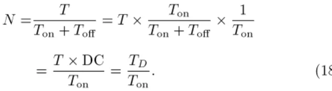
where DC is the duty cycle. On the other hand, the whole number of discharge pulses (N) during total machining time can be calculated as:
N =T T
on+ To = T
Ton
Ton+ To
1 Ton
= T DC Ton =
TD
Ton: (18)
Therefore, the total discharge energy (Q) during overall machining time is given by:
Q =q N = Vdis:Idis:TonTTD
on = Vdis:Idis:TD
= Vdis:Idis:T:DC: (19)
This is the total electrical discharge energy delivered into the gap zone, which is then shared between the tool and work piece electrodes, as well as the dielectric liquid. All the following discussions are based on this simple relation describing the whole generated electro-thermal energy during sparking, expressed in terms of the selected input EDM parameters. In what follows, a comprehensive parametric analysis of the inuence of input variables on output features is undertaken as main (direct) and interaction eect plots. In the rst, one factor is varied from the minimum to maximum level, while other parameters are kept constant at their
Figure 3. The main eects plot of input parameters over the MRR.
middle level. For the latter, the eect of a factor on the respective response is studied at dierent levels of another factor, while keeping all other variables unchanged.
4.1. Main eect analysis of MRR
In this section, the direct eects of four selected input factors, namely, A: discharge current, B: pulse on-time, C: duty cycle, and D: gap voltage on Material Removal Rate (MRR) are studied independently. The plots obtained in this manner are called main eects plots, which are discussed in the following.
Figure 3 shows the main eect plot of each variable on the MRR. As is clear, the MRR increases steadily with the increase of discharge current. Higher levels of discharge currents result in stronger electrical discharges capable of removing a chunk of material from the work piece, hence, boosting the rate of erosion [30]. The MRR tends to decrease with the increase of pulse on-time. Despite the usual belief that longer pulse on-times provide much more time for electrical discharging compared to shorter ones, in reality, longer pulse durations cause the plasma channel to expand excessively, thus, lowering the plasma
ush-ing eciency and electrical discharge density within the gap space, with more molten material resolidifying instead of being eectively removed [31,32]. On the contrary, the main eect of the duty cycle displays a reverse tendency. At a constant level of pulse on-time (B = 0), increasing duty cycle means lower-ing the pulse o-time, thereby, decreaslower-ing the idle time between successive sparks, which produces higher discharging frequency, leading to a higher removal rate. Finally, it can be inferred from the main eect plot of gap voltage that higher MRR is attainable at lower levels of gap voltage. Higher gap voltage provides wider gap distance, which, in turn, results in diminished electrical discharge density and larger gap electrical resistivity, hindering the proper trans-missivity of sparks [32]. So, the MRR decreases with the increase of gap voltage alone. It should be noted that these results have been acquired, considering the eect of each factor independently (keeping the other parameters unchanged). Nevertheless, more practically benecial outcomes are revealed when their mutual joint eects are investigated simultaneously. This can be obtained by studying interaction eect plots drawn for each signicant two-way interactive parameter over the relevant response.
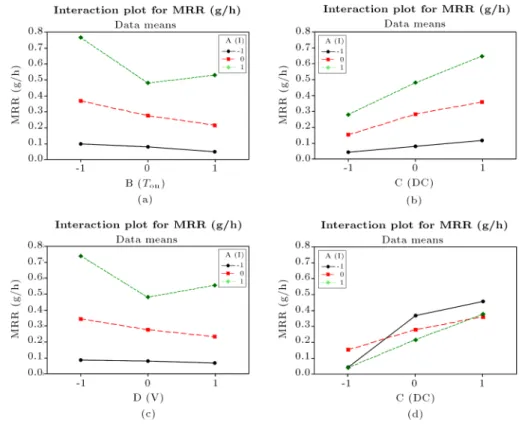
4.2. Interaction eect analysis of MRR
Figure 4(a) depicts the combined eects of pulse on-time at dierent levels of discharge current over the
MRR. It can be inferred that the maximum MRR is attainable at the lowest level of pulse on-time, along with the highest level of discharge current. This phenomenon can be best attributed to the increased energy density of discharge channel (J) relative to I and Ton, given by [33]:
J = kTIba
on; (20)
where a, b and k are constant coecients. Although the discharge energy itself is small with a short pulse on-time (Eq. 16), a higher discharge density is expected due to a very small discharge channel diameter. Hence, the higher the discharge current and the lower the pulse on-time, the larger is the electrical discharge density. Higher discharge density causes most of the material in the discharge area to be removed in the form of evaporation, with a thinner recast layer left on the work surface, increasing the plasma ushing eciency [34], hence, MRR. Figure 4(b) illustrates the interactive eect duty cycle and current on MRR. It is understood that while keeping pulse on-time and gap voltage constant, higher amounts of MRR are achievable at the point of both larger discharge current and duty cycle. At a steady pulse on-time, an increased duty cycle implies lower pulse o-time and, when combined with elevated discharge current, a higher rate of electrical discharge energy is assured, making the MRR as large as possible. Figure 4(c) shows the
Figure 4. Interaction eect plots of MRR: (a) Pulse on-time (B) and discharge current (A); (b): duty cycle (C) and discharge current (A); (c) gap voltage (D) and discharge current (A); and (d) duty cycle (C) and pulse on-time (B).
Figure 5. The main eects plot of input parameters over the TWR.
eect of gap voltage and current, whereas Figure 4(d) portrays the combined eect of duty cycle and pulse on-time over the MRR. It becomes clear that higher values of current, along with lower gap voltage, will denitely provide a suitable medium for higher rates of material melting and evaporation during sparking, thanks to enhanced electrical discharge density in a narrower gap region [31]. The lowest pulse on-time and highest duty cycle convey the greatest discharge frequency within the process input domain in which more material can be removed from the work piece in a unit time [35]. This event is clearly visible in Figure 4(d).
4.3. Main eect analysis of TWR
Figure 5 shows the main eect of each of four input parameters drawn, keeping the other factors constant at their middle level. A similar trend is observed compared to the main eects of MRR. The TWR tends to increase by increasing the discharge current and can reach up to about 0.09 g/h alone. This is the highest amount of TWR in these plots, which, in turn, conrms that the discharge current is paramount amongst other parameters in aecting the TWR. It is clear from the main eect plot of pulse on-time that setting longer pulse on-times can favor the TWR, as shorter pulse durations will deteriorate the tool wear. To better justify this fact, Figure 6 illustrates a schematic view of a single electrical discharge occurring between the two electrodes and the formed plasma channel. While keeping constant polarity, during every discharge, accelerated electrons bombard the surface of the anode (positive pole: tool), whereas ions aiming to move toward the cathode (negative pole: work piece) collide with the work surface. With small values of pulse duration, a higher number of negatively charged particles, being thousands of times lighter than ions, get the chance of being energized; stroking the positive (anode) tool electrode, and, thereby, increasing the rate of electrode material erosion [36,37]. On the same
Figure 6. Schematic drawing of a single electrical discharge.
basis, the rising tendency of TWR with regard to duty cycle can be rationalized. A higher level of duty cycle is equivalent to lower pulse o-time and, hence, higher pulse frequency, which implies greater TWR due to the privileged rate of electron collisions with the anode tool surface [30]. On the other hand, selecting lower gap voltage results in larger amounts of tool wear. The same reason as mentioned for the MRR can surely be applied here, since a larger gap distance, while keeping other variables unchanged, will give rise to reduced electrical discharge density, which can less aect the tool electrode against wear.
4.4. Interaction eect analysis of TWR
The interaction eect plot of TWR, with regard to current and pulse on-time, has been depicted in Fig-ure 7(a). As always smaller TWRs are demanded, they can be reached at lower discharge currents, followed by longer pulse on-times. A small discharge current provides lower discharge intensity (Eq. (16)), while prolonged pulse duration will give more chance for much heavier positive ions to reach the target cathode work piece, thus, occupying most of the plasma channel path and letting less excited electrons attack the anode tool [36].
Figure 7(b) shows the mutual eect of duty cycle and discharge current on TWR. It is noticeably re-vealed that smaller TWRs can, especially, be obtained by a combination of both low discharge current and duty cycle, and that much smaller TWRs are accom-plished moving towards the minimum current. This fact, however, cannot be elicited solely by checking the main eect plots of the duty cycle and current, as both
Figure 7. Interaction eect plots of TWR: (a) Pulse on-time (B) and discharge current (A); (b) duty cycle (C) and discharge current (A); (c) gap voltage (D) and discharge current (A); and (d) duty cycle (C) and pulse on-time (B).
present the same inuence on the TWR; increasing each of which makes the TWR increase progressively. This is undoubtedly due to the strong interactive nature of these two parameters suitably found by the ANOVA of TWR response (see Table 5). Moreover, the tool electrode suers more from wear, where both the current and duty cycle are chosen at their high levels; a point located at the upper right part of Figure 7(b). Increasing duty cycle at a steady level of pulse on-time (the case where Figure 7(b) has been drawn) means lowering the pulse o-time, thus, increasing the frequency of electrical discharge assuring higher rates of electron attack on the anode tool electrode in a unit time [36,37].
Figure 7(c) displays the interactive eect of gap voltage and current on the TWR. As can be inferred, low TWRs (less than 0.02 g/h) may be accessible with the smallest level of current (A = 1) accompanied by every adjustable level of gap voltage. In other words, the coincident eects of these two factors on TWR counteract the eect of gap voltage alone (shown in Figure 5), as now the whole range of it can be selected to yield small TWRs provided that the current is kept low enough (A = 1). Figure 7(d) shows the concurrent eect of duty cycle and pulse on-time. It is obviously visible that small TWRs (below 0.03 g/h) can be obtained choosing the lowest level of duty cycle (C = 1) with a range of medium to high levels of pulse on-time (0 < B < 1). This combination conrms
Figure 8. The main eects plot of input parameters over the Ra.
relatively decreased sparking frequency, meaning lower amounts of electron attack in a unit time to cause tool wear [36,37].
4.5. Main eect analysis of Ra
Figure 8 depicts the main eects plot of the four controllable parameters on the Ra. It is understandable that the rst two variables, current and pulse on-time, have more inuential impacts on the Ra than those of duty cycle and gap voltage. More specically, increasing pulse on-time alone, while keeping the other factors constant at their middle levels, can increase the
Ra from 4 m up to about 5.7 m; a higher dierence interval than that created by other parameters. As is also clear, altering both duty cycle and gap voltage, within their designated intervals considered in this research, causes little change of the Ra. This fact was also veried before (see Table 5), as not being signicant parameters within 95% of condence inter-val, and their main eects have just been shown here for comparative purposes. In general, the work surface quality in EDM depends primarily on the magnitude of electrical discharge energy governed mainly by current intensity and pulse on-time [31,32]. A prolonged pulse on-time makes the discharging action continue for a longer duration, so that broader craters are formed over the work surface, overwhelmed with an abundance of resolidied molten material not ejected eectively. This, in turn, leads to worsened and coarser surface quality [13].
4.6. Interaction eect analysis of Ra
Figure 9(a) illustrates the joint eects of pulse on-time and discharge current over the Ra. It is apparent that smoother surfaces can be obtained by assigning the lowest level of pulse on-time (B = 1), while providing a fair amount of discharge current. For example, if it is desired to produce a surface having a Ra roughness less than about 4 m, then, it is feasible to choose any arbitrary value for the discharge current, within its investigated domain, provided that the pulse on-time is kept at its lowest level (B = 1). More noticeably, the combination of B = 1 and A = 0 gives the lowest Ra. Enough discharge current is needed to remove material from the high melting point WC-Co composite more eectively, with less remaining recast layer over the work piece, worsening the surface quality [31,32]. Figure 9(b) portrays the two-way interaction eects of gap voltage and discharge current. Under the circumstances in which this graph has been drawn, it can be concluded that the lowest value of Ra (about 4.2 m) is achieved setting the highest level of gap voltage (D = 1), along with
the minimum level of discharge current (A = 1). Higher gap voltage, while making the gap distance wider, facilitates debris removal from the gap space and can also help reduce electrical discharge density. Altogether, with low current intensity, they collaborate in attaining a superior surface quality [31,32].
5. Optimum selection of EDM parameters on WC/6%Co using desirability function technique
Metal removal rate is an indicator for productivity, while tool wear rate and surface nish account for process economics, precision, and work quality. In particular, tool wear is of paramount concern, espe-cially when close tolerances in intricate geometries are needed. The EDM, as a complex and stochastic pro-cess, exhibits much diculty in determining optimal machining parameters for best machining performance. The performance indicators, viz. MRR, TWR and Ra, are conicting in nature, as it is always desirable to have higher MRR, with a lower value of surface roughness and tool wear rate, at the same time. Due to the presence of a large number of process variables and mutual interactions, the selection of optimum machin-ing parameter combinations, to obtain higher MRR and smaller SR and TWR, is a challenging task [38]. Here, an attempt is made to develop a strategy based on the concept of desirability function for predicting the optimum machining parameter settings, generating maximum MRR, with minimum SR and TWR, all at once.
5.1. Optimization formulation
The mathematical formulation of the present optimiza-tion problem can be stated as follows:
Max : F1(x) = MRR;
Min : F2(x) = TWR;
Min : F3(x) = Ra:
Figure 9. Interaction eect plots of Ra: (a) Pulse on-time (B) and discharge current (A); and (b) gap voltage (D) and discharge current (A).
Subject to : 2 x1 8
50 x2 150
40 x3 80
40 x4 80; (21)
where x1, x2, x3 and x4 represent the input process
parameters, I, Ton, DC and V , respectively. It is a
four-variable-three-objective optimization statement, each of which has been dened by its respective second order regression equation (Eqs. (13)-(15)).
5.2. Optimization through desirability function Popularized by Derringer and Suich [39], the Desir-ability Function Approach (DFA) is a kind of search-based optimization method capable of handling several response functions simultaneously to nd optimal input settings, globally. The overall approach is to rst convert each response, yiinto an individual desirability
function, di, that varies over the range:
0 di 1: (22)
If the response yi is at its goal or target, then di = 1
(the most desirable case), and if the response is outside an acceptable region, then, di = 0 (the least desirable
case). There is also a positive number, weight factor (r), associated with the desirability function of each response dening its shape. If the weight is chosen to be less than 1, then the sensitivity of the desirability function is low with respect to the optimal or target value sought for. In other words, if the search algorithm nds a point which is somehow far from the desired optimum or target value, then the decrease in desir-ability function value will be small in comparison to its maximum amount (unity). Choosing a weight factor higher than one has the reverse eect, and setting it to one provides a balanced or medium sensitivity with the shape of desirability being linear [24,25,40]. The individual desirability functions are dened according to the goal of optimization, i.e. maximization or minimization.
If the objective or target, Ti for the response, yi,
is a maximum value, then:
di=
8 > > > < > > > :
0 yi Li
yi Li Ti Li
r
Li yi Ti
1 yi Ti
(23)
and if the target for the response is a minimum value, then:
di=
8 > > > < > > > :
1 yi Ti
Ui yi Ui Ti
r
Ti yi Ui
1 yi Ui
(24)
where Li and Ui represent the lower and upper limit
values of the response, yi, respectively.
The individual desirabilities are then combined to form the overall (composite or aggregated) desirability (D), another parameter varying between 0 and 1, as the weighted geometric mean of all the previously dened desirability functions, given by:
D = (dw1
1 dw22 dw33 ::: dwnn)
1 (w1+w2+w3+:::+wn)
= (n i=1dwii)
1 Pn
i=1 wi ; (25)
where wi is of relative importance, a comparative scale
for weighing each of the resulting di assigned to the
ith response, and n is the number of responses (n = 3, in our case). The optimal settings are determined, so as to maximize overall desirability (D), usually by applying a reduced gradient algorithm with multiple starting points [40].
5.3. Parametric optimization of the EDM process on WC-6%Co
Based on the developed quadratic mathematical re-sponses (Eqs. (13)-(15)), d1, d2, and d3 are selected
as the independent desirability functions for the MRR, TWR, and Ra, respectively. Moreover, the targets are placed on the MRR to become maximized, while TWR and Ra to be minimized. Unit weight factor (r = 1) and importance (wi = 1) were also assigned
for each response. The Response Optimizer option within the DOE module of the Minitab statistical software package, release 15, has been used here to search for the best set of optimum input parametric combinations, resulting in the most desirable compro-mise between dierent responses. Table 10 summarizes the key parameters set to nd global optimum settings, including constraints of input variables and that of
Table 10. Constraints and criteria of input parameters and responses.
Parameter/Response Goal Lower limit
Upper limit Discharge current In range 2 8
Pulse on-time In range 50 150
Duty cycle In range 40 80
Gap voltage In range 40 80 Material removal rate Maximize 0.02 0.86
Tool wear rate Minimize 0.007 0.15 Surface roughness Minimize 3.395 6.589
Table 11. Iterative determination of optimum conditions (inputs in coded form). Solution Current
(A)
Pulse on-time
(B)
Duty cycle (C)
Gap voltage
(D)
MRR (g/h)
TWR (g/h)
Ra
(m) d1 d2 d3
Composite desirability
(D)
1 0.232323 -0.989478 -1 -1 0.30187 0.04241 3.89837 1 1 1 1
2 0.434343 -0.959596 -1 -0.959596 0.33782 0.05002 3.89841 1 0.999604 1 0.999868
3 -0.397059 -1 1 1 0.3 0.04763 3.94184 1 1 0.961959 0.987155
4 -0.501927 -0.942816 1 -1 0.32798 0.05 4.06218 1 1 0.852562 0.948219 5 0 -1 0 0.881845 0.3 0.05158 4.07341 1 0.96846 0.842356 0.934385 6 0.643528 -1 0.930431 0.419331 0.28849 0.05 4.16654 0.88494 0.999984 0.75769 0.875251 7 0.43614 -1 -0.599353 0.970432 0.27956 0.05 4.23107 0.79558 9 0.999998 0.699026 0.822357 8 -0.157129 -0.476585 1 1 0.32588 0.05 4.44991 1 1 0.500078 0.793742 9 0.997587 -1 -1 1 0.27054 0.0564 4.43547 0.705421 0.8719 67 0.513207 0.680895 10 0.344275 -0.15463 -0.946309 -1 0.28279 0.04136 4.64325 0.827884 1 0.324322 0.645132
Note: The rst row in italic is selected as the best compromise solution.
response requirements, while Table 11 sorts the rst ten optimum settings obtained in descending order of composite desirability (D). The closer D is to 1, the more favorable are the EDM conditions satisfying prob-lem requirements. It can be seen from Table 11 that the most desirable operating conditions correspond to the rst row and are discharge current A = 0:2323, pulse on-time B = 0:9895, duty cycle C = 1 and gap voltage D = 1 in coded form, equivalent to 5:70A, 50.53 s, 40% and 40 V as real values, respectively. Accordingly, the optimized responses are 0.302 g/h, 0.042 g/h, and 3.898 m for MRR, TWR, and Ra, respectively. A closer examination of the whole listed settings in Table 11 reveals that although higher MRRs can be obtained by other settings, those cases are subject to sacricing both TWR and Ra, as they obtained higher values than those pertinent to the rst solution. Figure 10 illustrates a visual representation
Figure 10. Final optimization results.
of the optimization result. The optimization plot shows the eect of each factor (columns) on the re-sponse or composite desirability (rows). Furthermore, each cell presents how the process output varies as a function of one of the process factors, while keeping the other parameters unchanged. Also, the vertical lines inside the cells show current optimal parametric settings, whereas the dotted horizontal lines represent the current response values. High and low settings of each process design variable can also be observed in this plot, denoted by 1 and -1, respectively. The most useful part is the optimal parameter settings required to achieve the process set target criteria, located in the middle row between the high and low rows, symbolized by \cur" and expressed in coded form. Finally, the rst left column shows the composite, as well as all individual desirability, all being unity, along with optimum response values.
Conducting the conrmation experiment is the crucial, nal, and indispensable part of every optimiza-tion attempt. A vericaoptimiza-tion experiment was performed at the obtained optimal input parametric setting to compare the actual MRR, TWR, and Ra with those of optimal responses obtained through a desirability approach. Table 12 summarizes the optimization results, along with experimentally obtained responses, and their relative percentage verication errors.
As is clear, the amounts of error are all found to be satisfactory, from the point of engineering applications (10.64% as the worst case) in predicting the TWR, assuring the feasibility, predictability, and eectiveness of the adopted approach.
Moreover, these error values are also in good agreement with those represented in Table 9, all be-ing in a comparable error margin for each response, proving that a consistent and reliable strategy has been employed in this research.
Table 12. Multi-response optimal points and experimental validation. Optimum
input setting
MRR (g/hr)
TWR (g/hr)
Ra (m)
Relative prediction
error (%) I
(A) Ton
(s) DC (%)
V
(V) Predicted Exp.
a Predicted Exp.a Predicted Exp.a MRR TWR Ra
5.70 50.53 40 40 0.302 0.331 0.042 0.047 3.898 4.141 8.76 10.64 5.87
a: Experimental.
5.4. The interpretation of optimal settings Making a thorough analysis of the optimum input values can provide a fair basis to justify their estimated amounts from the point of physical aspects involved in the EDM process. In the course of optimization through the desirability function approach, a measure of how well the solution has satised the combined goals for all responses must be assured. That is, D = 1, and the optimum setting providing this could have been able to make a tradeo between dierent objective functions. The amount of optimal discharge current has been found to be near its middle value, providing fair electro-thermal energy, so that neither a very low MRR nor an extremely high one is obtained. Along with almost the shortest possible pulse on-time (50.53 s), the existence of adequate electrical discharge density is assured to help maintain enough impulsive force to expel much of the molten material from the crater [38,11]. Moreover, as was discussed in subsection 4.5, shorter pulse on-times are in favor of smoother surfaces, as the resulted craters' dimensions (depth and diameter) are smaller compared with those created with long pulse durations. Hence, better sur-face quality is guaranteed. Finally, the optimal values of duty cycle and gap voltage are equivalent to their lowest possible levels considered in the experimental plan, as increasing either of them may cause the process performance to deviate from its optimum condition by sacricing any of the three responses. This eect can be seen in Table 11. Especially, the lowest gap voltage (40 V) provides a narrower gap distance, increasing the electrical discharge density inside the gap zone, which, in turn, helps improve the MRR.
6. Conclusions
Conventional machining of the hard metal WC/6%Co composite is extremely laborious, burdensome, and time consuming, due to its elevated hardness and brit-tleness over a wide range of temperatures and working conditions. The eective and economic utilization of the EDM process on such a material, with optimum selection of input parameters, needs a thorough under-standing of its machinability behavior, which, in turn, can substantially alleviate the diculties encountered. In short, based on in-depth and comprehensive analysis
and optimization of WC-6%Co ED-machinability in-dices, the following principal conclusions can be drawn:
1. All the main eects of input parameters, i.e. dis-charge current, pulse on-time, duty cycle and gap voltage, have been found to be highly signicant, aecting both the MRR and TWR. However, for the third response, Ra, just the main eects of the rst two were revealed to be statistically important.
2. Regarding the main eects analysis, both the MRR and TWR behave in the same way. However, the TWR behaves more nonlinearly. Increasing either discharge current or duty cycle results in higher values of stock removal rate and tool wear, whereas increasing pulse on-time or gap voltage causes the reverse eect. On the other hand, the work roughness value, Ra, is directly proportional to both the discharge current and pulse on-time, while the main eects of the other parameters were found to be negligible.
3. The two way interaction eects of discharge current with pulse on-time (A B), duty cycle (A C), and gap voltage (A D), as well as the interaction between the pulse on-time with duty cycle (B C) and pure quadratic eect of duty cycle (C2), have
all been found to signicantly inuence the MRR.
4. On measuring TWR, the same dual interaction ef-fects inuencing the MRR, plus the pure quadratic eect of discharge current (A2), were understood to
be statistically signicant.
5. For the Ra response, the interactions between discharge current with pulse on-time (A B) and discharge current with gap voltage (A D) possess signicant eects.
6. Higher MRRs are always accessible through either enhancing electrical discharge density or rising sparking frequency. These conditions are feasible by lowering the pulse on-time and gap voltage or increasing duty cycle, while considering larger dis-charge currents to conrm greater released electro-thermal energy as a result of sparking.
7. Low amounts of TWR can mainly be obtained by a combination of lower current levels with prolonged pulse on-times or longer pulse on-times