Fuzzy Hierarchical Queueing Models
for the Location Set Covering
Problem in Congested Systems
H. Shavandi
1and H. Mahlooji
In hierarchical service networks, facilities at dierent levels provide dierent types of service. For example, in health care systems, general centers provide low-level services, such as primary health care, while specialized hospitals provide high-level services. Because of the demand congestion at service networks, the location of servers and their allocation of demand nodes can have a strong impact on the length of the queue at each server, as well as on the response time to service calls. This study attempts to develop hierarchical location-allocation models for congested systems by employing a queueing theory in a fuzzy framework. The parameters of each model are approximately evaluated and stated as fuzzy-numbers. The coverage of demand nodes is also considered in an approximate manner and is stated by the degree of membership. Using queueing theory and fuzzy conditions, both referral and nested hierarchical models are developed for the Location Set Covering Problem (LSCP). To demonstrate the performance of the proposed models, a numerical example is solved in order to compare the results obtained from the existing probabilistic models and the new fuzzy models developed in this paper.
INTRODUCTION AND LITERATURE REVIEW
There exist many hierarchical structures in service networks, both in the public and private sectors. Here, some examples of hierarchical service networks are elaborated on. Public health services are, by nature, hierarchical structures, as hospitals correspond to higher-level facilities and primary health care centers are thought of as at a lower level. Numerous other examples of hierarchical structures can be found, such as primary, middle and high schools [1], airports, computer service centers, day-care centers, health care systems, emergency medical centers, regional health facilities, social service centers, police centers, ware-houses, distribution systems and so on. Due to the nature of the relationship between the various levels, both on the demand side as well as the service side, the analysis of hierarchical service systems is a challenge waiting to be met.
1. Department of Industrial Engineering, Sharif University of Technology, Tehran, Iran.
*. Corresponding Author, Department of Industrial Engi-neering, Sharif University of Technology, Tehran, Iran. E-mail: [email protected]
This research eort is devoted to the development of fuzzy models for the hierarchical Location Set Cov-ering Problem (LSCP). LSCP, which was introduced by Toregas et al. [2], attempts to locate the minimum number of servers, in order to cover all the demand nodes within the distance or time standard.
Church and Eaton [3] and Gerrard and Church [4] provide reviews of early hierarchical models. Serra and ReVelle [5,6] combined hierarchical location and coherent districting in a later eort. Serra et al. [7] developed a hierarchical maximum capture model for location in a competitive environment. Later, Serra [8] presented his model for a coherent covering location problem.
The assumption of demand congestion at servers has not been considered in any of the above models. Once the demand rate (for service) exceeds the service rate, congestion occurs and waiting lines emerge. To enhance the quality of rendering service in congested systems, it is obvious that resorting to a queueing theory could be quite helpful. Marianov and Serra [1] published an article on hierarchical location-allocation models for congested systems (HIQ-LSCP), in which they developed a number of hierarchical location mod-els for LSCP and MCLP, based on the queueing theory. The probabilistic nature of their approach led to more
models under crisp conditions. In fact, to make the models even more realistic, one can consider the fuzzy conditions. As for the application of fuzzy theory toward developing location models, most eorts can be categorized into a class of qualitative models. In 1999, Canos et al. [9] treated the classical p-median problem as a fuzzy model and came up with an exact method of solution. Woodyat et al. [10] presented an application combining set covering and fuzzy sets to optimally assign metallurgical grades to customer orders. A comprehensive review of newly developed hierarchical location models can be found in [11]. The very rst fuzzy model using the queueing theory in the area of location-allocation in congested systems was developed by Shavandi and Mahlooji [12]. They incorporated fuzzy parameters and variables in their work. In their model, no customer is required to receive service from a single server; rather, he can select the appropriate server with priorities from a list of servers, according to degrees of membership. The rst fuzzy model for location-allocation in hierarchical systems was developed by Shavandi et al. [13]. They introduced a fuzzy hierarchical queueing location-allocation model for MCLP in coherent systems. Shavandi and Mahlooji developed a fuzzy queueing maximal covering location-allocation model with a genetic algorithm in 2006 [14]. The present work follows the aim of developing fuzzy hierarchical queueing models for LSCP, in both nested and referral systems.
A REVIEW OF PROBABILISTIC HIERARCHICAL LOCATION SET COVERING PROBLEM (HIQ-LSCP)
To lay the foundation for presenting the Fuzzy Hierar-chical Queuing Location Set Covering Problem (FHQ-LSCP), it is appropriate to review the HIQ-LSCP model for referral systems proposed by Marianov and Serra [1], which is as follows:
min Z =X
j
CjWj+
X
k
KkZk; (1)
s.t. X
j;k
Xijk = 1; 8i; (2)
Xijk Wj; 8i; j; k; (3)
Xijk Zk; 8i; j; k; (4)
P [low-level server j has b people in queue] ;
8j; (5)
P [high-level server k has b people in queue] ;
8k; (6)
Xijk; Wj; Zk = 0; 1; 8i; j; k;
where:
Xijk: The allocation variable that takes a value
of 1, if the population at demand node i is allocated to the low-level server, j, and the high-level server, k; otherwise it is zero, Wj: The location variable, which takes a value
of 1, if a low-level server is located at node j, otherwise it is zero,
Zk: The location variable that takes a value
of 1, if a high-level server is located at node k, and zero otherwise,
Cj: The cost of locating a low-level server at
node j,
Kk: The cost of locating a high-level server at
node k,
The objective function (Equation 1) attempts to minimize the total cost of locating low- and high-level servers. The rst constraint (Equation 2) means that each demand node must be covered by just one server. Constraints 3 and 4 assume that allocation variables can take the value 1, only when a low-level server and a high-level server have already been located at nodes j and k, respectively. Constraints 5 and 6 are related to the demand congestion at servers, or the quality of service, to make sure that the queue length at each server does not exceed b, with probability at least .
To write Constraints 5 and 6 in non-probabilistic form, Marianov and Serra borrow notions from the queueing theory to arrive at the nal form for these constraints as follows:
X
i;k
fiXijk ljb+2
p
1 ; 8j; (50)
or: X
i;j
jfiXijk hkb+2
p
1 ; 8k; (60)
where the following denitions are relevant: fi: The arrival rate of requests for service at
node I, l
j: The service rate at low-level server j,
h
k: The service rate at high-level server k,
j: The percentage of requests referred by the
low-level server, j, to high-level service. They assume that, at each service center, there exists just one server. Since each demand node is served
by just one server, the servers operate independently and the queueing model at each server functions as an M/M/1 model. So, by substituting Constraints 50
and 60 for 5 and 6, they arrive at the nal form of the
HIQ-LSCP model.
FUZZY HIERARCHICAL QUEUEING LOCATION SET COVERING PROBLEM (FHQ-LSCP)
This section is devoted to the development of two types of FHQ-LSCP model. First, a fuzzy hierarchical queueing location set covering formulation for referral systems is presented, which can easily be applied to non-referral systems as well. Then a similar model is developed for a nested system. In the case of nested systems, a server providing both high-level and low-level services is modeled as a low-level server co-located with a high-level server. First, the parameters, variables and fuzzy sets are dened that are used in developing such models. In the following discussion, the convention is adopted of referring to a node in the service network as a service node (or a server), if a server is located at that node. Otherwise, the node is simply referred to as a demand node. The parameters are as follows:
Cj: The cost of locating alow-level server at node j;
a crisp number,
Kk: The cost of locating a high-level server at node
k; a crisp number,
~bl: (bpl; bml ; bol): A triangular fuzzy number, which
stands for the maximum allowable number of customers at each low-level server,
~bh: (bph; bmh; boh): A triangular fuzzy number, which
stands for the maximum allowable number of customers at each high-level server, ~
fi: (fip; fim; fio): A triangular fuzzy number,
which stands for the low-level demand rate at demand node i,
: The high-level demand percentage at each low-level server, a crisp number,
~l
j: (lpj ; lmj ; loj ): Service rate at low-level
server j; a triangular fuzzy number, ~h
k : (hpk ; hmk ; hok ): Service rate at high-level
server k; a triangular fuzzy number, sdl
ij: The degree of membership for the distance
between demand node i and the low-level server, j, being almost less than or equal to the distance standard,
slh
jk: The degree of membership for the distance
between the low-level server, j, and the high-level server,
k, being less than or equal to the distance standard,
: The predened truth-value of service quality constraint at each server,
m: The minimum degree of membership by which each demand node must be covered; a crisp number.
The variables are categorized into variables and deci-sion variables. The variables are functions of decideci-sion variables and are only used to model the problem. As such, the variables do not appear in the nal model. In light of this denition, the variables are as follows:
~ NSl
j : The average number of customers at low-level
server j during the steady state period; a triangular fuzzy number,
~ NSh
k : The average number of customers at
high-level server k during the steady state period; a triangular fuzzy number, ~l
j : (lpj; lmj ; loj ): Arrival rate of demand at
low-level server j; a triangular fuzzy number, ~h
k : (hpk ; hmk ; hok ): Arrival rate of demand at
high-level server k; a triangular fuzzy number. The decision variables of the proposed models are as follows:
Wj: A zero-one variable, which assumes a value
of 1 if a low-level server is located at node j, otherwise, it is zero,
Zk: A zero-one variable, which assumes a value
of 1, if a high-level server is located at node k, otherwise, it is zero,
Xij: The degree of membership for demand node
i being covered by the low-level server, j, Yjk: The degree of membership for referring
high-level services from the low-level server, j, to the high-level server, k.
The fuzzy sets that are used in the models are as follows:
~ Ndl
j : This discrete fuzzy set represents the distance of
all demand nodes from low-level server j and is dened as follows:
~ Ndl
j =
( sdl
1j
1 ; sdl
2j
2 ; ; sdl
ij
i )
; 8j;
where sdl
ij stands for the degree of membership for
the distance between demand node i and the low-level server, j, to be approximately smaller than or equal to the distance standard and is calculated as follows.
Let dij represent the distance between demand
node i and the low-level server, j. Also, let sdl denote
the distance standard for low-level services. Now, the statement \the demand node i's distance from the low-level server, j, is approximately less than, or equal to the distance standard", can be represented by the following fuzzy notation:
Such a denition makes it possible to put any demand node, i, in the set, ~Ndl
j , for the low-level server, j,
according to its degree of membership. The degree of membership, sdl
ij, can be calculated as:
sdl ij = 8 > < > :
0; dij > udl udl dij
udl sdl; sdl dij < udl
1; dij sdl;
(8)
where udl stands for the acceptable upper bound for
the distance standard. Relation 8 is obtained based on Figure 1.
Thus, the set, ~Ndl
j , is dened as a fuzzy set as:
~ Ndl j = ( sdl 1j 1 ; sdl 2j
2 ; ; sdl
ij
i ; )
; 8j;
where each demand node belongs to set ~Ndl
j , according
to a degree of membership. ~
Ndl
k : This discrete fuzzy set represents the distance of
the low-level servers from the high-level server, k, and is dened as:
~ Nlh k = ( slh 1k 1 ; slh 2k
2 ; ; slh
jk
j )
; 8k:
The technicalities in evaluating slh
jkare similar to those
in the evaluation of sdl ij.
~ Cdl
j : This fuzzy set includes the demand nodes, which
are approximately covered by the low-level server, j, i.e: ~ Cdl j = X1j 1 ; X2j
2 ; ; Xij i ; 8j: ~ Clh
k : This fuzzy set includes the low-level servers, which
are approximately covered by the high-level server, k, for referring the high-level services, i.e:
~ Clh k = Y1k 1 ; Y2k
2 ; ; Yjk
j
; 8k:
Figure 1. The membership function of the distance standard.
In this work, it is intended to develop models, which cover the demand nodes that are within the distance standard. Thus, for the case of low-level servers, one has to nd the intersection of the fuzzy sets, ~Cdl
j and
~ Ndl
j , to determine the issue of coverage for the demand
nodes, with respect to the distance standard. As such, a new fuzzy set is obtained whose elements consist of the common elements of the two sets. The degree of membership for each element in this set is equal to the minimum of the degree of membership for the same element across the two fuzzy sets. So, if the condition that Xij never exceeds sdlij is included, then,
the coverage of low-level services will be within the distance standard. The same conditions are needed to ensure that the coverage of high-level services stays within the distance standard, as well. Therefore, the following constraints must be added to the model:
Xij sdlij; (9)
Yjk slhjk: (10)
~ Dl
j: This is the set of demands that are approximately
covered by the low-level server, j, i.e:, ~ Dl j = X1j ~ f1 ;
X2j
~ f2 ; ;
Xij
~ fi
; 8j: (11)
Each element of this set is a triangular fuzzy number. In the following section, this set is employed to deter-mine the arrival rates of the service demands for the low-level servers.
~ Dh
k: This is the set of high-level services referred to by
the low-level servers; services which are approximately covered by the high-level server, k, i.e:
~ Dh k = ( Y1k l 1; Y2k l 2; Yjk l j; )
; 8k: (12)
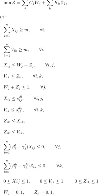
Mathematical Model for Referral FHQ-LSCP The FHQ-LSCP mathematical model for the referral systems, which is a mixed integer programming model, is as follows:
min Z =X
j
CjWj+
X
k
KkZk; (13)
s.t.:
n
X
j=1
Xij m; 8i; (14)
n
X
k=1
Xij Wj; 8i; j; (16)
Yjk Zk; 8j; k; (17)
Yjk Wj; 8j; k; (18)
Xij sdlij; 8i; j; (19)
Yjk slhjk; 8j; k; (20)
~ NSl
j ~bl; 8j; (21)
~ NSh
k ~bh; 8k; (22)
0Xij 1; 0Yjk 1; Wj=0; 1; Zk=0; 1:
The objective Function 13 attempts to minimize the cost of locating the low- and high-level servers for approximately covering all the demand nodes. Con-straint 14 guarantees that all demand nodes must be covered by the low-level servers having the least degree of membership, m, while Constraint 15 ensures that level services must be covered by the high-level servers having the least degree of membership, m. The purpose of Constraints 16 to 18 is to assure that, unless a server is located at a node, the other demand nodes cannot be covered by that node's server. Constraints 19 and 20 have been explained before. Finally, Constraints 21 and 22 have to do with the quality of rendering service by the low- and high-level servers. They enforce the condition that the average number of customers for each server stays less than, or equal to a given value (~blor ~bh).
The average number of customers for each server is obtained as a triangular fuzzy number; an issue which will be elaborated on later. The maximum permissible number in the system is also a triangular fuzzy number. Accordingly, in Constraints 21 and 22, a triangular fuzzy number must be less than or equal to another triangular fuzzy number. To include such a constraint, the method proposed by Dubois and Prade [15] is adopted. According to this method, the correctness of the intended inequality holding true must be calculated. In fact, for any two fuzzy numbers, ~Iand
~
J, the correctness of ~I ~J holding true is calculated as:
T (~I ~J) = supfminfI~(x); J~(y)gg; (23)
where I~(x) and J~(y) represent the membership
functions for x belonging to ~I and y belonging to ~J. Following this convention, Constraints 21 and 22 are converted into:
T ( ~NSl
j ~bl) 1 ; (24)
and: T ( ~NSh
k ~bh) 1 : (25)
Now the procedure for calculating ~NSl
j for low-level
servers is presented and, then, using the results, the average number of customers at high-level servers, ( ~NSh
k ), is obtained. In order to calculate ~NjSl, one
begins with calculating the arrival rate of service demand to the low-level servers.
The set of service calls covered by server j was initially dened as:
~ Dl
j =
X1j
~ f1 ;
X2j
~ f2 ; ;
Xij
~ fi
; 8j:
Since ~fi, in this fuzzy set, is covered by the
low-level server, j, with a degree of membership equal to 1 and the set itself is convex, then, ~Dl
j becomes a
discrete fuzzy number. To evaluate ~l
j, the centroid
method [16,17] is employed, which is intended for transforming a fuzzy number into a classical (crisp) number. This method, however, will transform ~Dl
j to
a triangular fuzzy number, because the elements of ~Dl j
are all triangular fuzzy numbers.
To employ the centroid method, let ~Z stand for a discrete fuzzy number, such as:
~ Z =
~c(z1)
z1 ;
~c(z2)
z2 ; ;
~c(zi)
zi
;
where crisp numbers, zi, are elements of ~Z and ~c(zi)
represents zi's degree of membership in ~Z. Using the
centroid method, the fuzzy number, ~Z, is transformed to the crisp number, Z, as:
Z=
P
iP~c(zi)zi i ~c(zi)
: (26)
Now, using Equation 26, the fuzzy number, ~Dl j, is
transformed to a triangular fuzzy number, (~l j), as:
~l j =
P
i
~ fiXij
P
i Xij
; 8j: (27)
Since ~fi's are triangular fuzzy numbers, the fuzzy
number obtained from Equation 27 is also a triangular fuzzy number in the form of:
~l
j = (lpj ; lmj ; loj); 8j; (28)
lpj = P
i f p iXij
P
i Xij
; lm
j =
P
i f m i Xij
P
i Xij
; lo j =
P
i f o iXij
P
i Xij
:
In a similar manner, using Equation 26, the fuzzy number, ~Dh
k, is transformed into a triangular fuzzy
number, (~h k), as:
~h k =
P
j ~ l jYjk
P
j Yjk
; 8k;
that is the arrival service rate to high-level server k. There is also:
~h
k = (hpk ; hmk ; hok ); 8k; (29)
where: hp k = P j lp j Yjk
P
j Yjk
; hm
k =
P
j
lm j Yjk
P
j Yjk
; ho k = P j lo jYjk
P
j Yjk
:
Due to the fact that the demand for service at each demand node follows a Poisson process, the service calls' arrival rate to server j also obeys a Poisson process. It is assumed that server j's service time follows an exponential distribution with parameter ~l
j.
Since the parameters of such distributions are fuzzy in nature, the queueing model at each server will be an FM/FM/1 model (FM Fuzzy Markovian). Now, to evaluate ~NSl
j , the fuzzy Little relations are used, which
are proposed by Jo et al. [18], i.e:
~ NSl j = ~l j ~l j ~lj
: (30)
Since ~l
j and ~lj are triangular fuzzy numbers, ~NjSl,
obtained from Equation 30 also be a triangular fuzzy number, i.e:
~ NSl
j = (NjSlp; NjSlm; NjSlo); (31)
where:
NjSlp=
P
i f p iXij
lo
j P
i Xij
P
i f o iXij;
NSlm
j =
P
i f m i Xij
lm j
P
i Xij
P
i f m i Xij;
NSlo
j = i
fo iXij
lpj P
i Xij
P
i f p iXij:
Reasoning in a similar manner, the average number in the system for high-level servers, ~NSh
k , is obtained as:
~ NSh
k = (NkShp; NkShm; NkSho); (32)
where: NShp k = P j lp j Yjk
ho k
P
j Yjk
P
j
lo jYjk;
NShm
k =
P
j
lm j Yjk
hm k
P
j Yjk
P
j
lm j Yjk;
NSho
k =
P
j
lo j Yjk
hpk P
j Yjk
P
j
lp j Yjk
:
By writing Constraints 21 and 22 in deterministic form, the model is converted to a mixed integer programming model. To make this possible, the following lemma is used that is proven in [12].
Lemma
Given two triangular fuzzy numbers, ~I = (Ip; Im; Io)
and ~J = (Jp; Jm; Jo), one has:
a) T (~I ~J) = 1 , Im Jm; (33)
b) T (~I ~J)1 ,ImJo (1 )(Jo Jm): (34)
On the basis of Relation 34, one can transform Con-straint 21 to a linear form as:
T ( ~NSl
j ~bl)1 NjSlmbol (1 )(bol bml ):
(35) By substituting the equivalent of NSlm
j from Equation
31 and doing appropriate mathematical manipulations, one will arrive at the following linear form:
n
X
i=1
('l
i jl)Xij 0; 8j; (36)
where: 'l
i= fim+ bolfim (1 )(bol bml )fim; 8i; (37)
l
Constraint 22, in turn, will be transformed into the following form:
n
X
j=1
('h
j hk)Yjk 0; 8k; (39)
where: 'h
j = lmj + bohlmj (1 )(boh bmh)lmj ; 8j;
(40) h
k = bohhmk (1 )(bho bmh)hmk ; 8k: (41)
Therefore, the nal referral FHQ-LSCP model can be written as:
min Z =X
j
CjWj+
X
k
KkZk;
s.t.:
n
X
j=1
Xij m; 8i;
n
X
k=1
Yjk mWj; 8j;
Xij Wj; 8i; j;
Yjk Zk; 8j; k;
Yjk Wj; 8j; k;
Xij sdlij; 8i; j;
Yjk slhjk; 8j; k; n
X
i=1
('l
i jl)Xij 0; 8j;
n
X
i=1
('h
i hk)Yik 0; 8k;
0 Xij 1; 0 Yjk 1; Wj=0; 1; Zk=0; 1:
FHQ-LSCP for the Nested Systems
In the nested hierarchical systems, the high-level servers are capable of rendering service at lower levels as well, while the low-level servers oer low-level services only. Since, for the purpose of developing the model, all the parameters dened, previously, are still valid, just the variables and the fuzzy sets are dened.
The decision variables for the nested FHQ-LSCP are as follows:
Xij: The degree of membership for the demand
node, i, to be covered by the low-level server, j.
Vik: The degree of membership for the demand
node, i , to be covered by the high-level server, k.
The variables Wjand Zkhave the same interpretations
as before. Likewise, except for the fuzzy sets of demands covered by the high-level servers, the other sets are dened as before. To dene the fuzzy set of demands covered by the high-level servers in the nested system, the reasoning is as follows.
From each demand node i, two calls for service with dierent degrees of membership arrive at the high-level server, k. The low-high-level service, with rate ~fi, is
covered by the high-level server, k, with the degree of membership, Xik. The high-level service, with rate
if~i, is covered by the high-level server, k, with the
degree of membership, Vik. On the basis of the fuzzy
algebraic relations, these rates can be added together with the sum having a degree of membership equal to the minimum of (Xik, Vik). Thus, one needs to dene
the variable, Zik, as follows:
Zik: The degree of membership for demand node i to be
covered by the high-level server, k, which covers both low-level and high-level services, i.e:
Zik= min(Xik; Vik): (42)
The fuzzy set of demands, which are approximately covered by the high-level server, k, is dened as follows:
~ Dh
k =
z1k
~
f1+ 1f~1;
z2k
~
f2+ 2f~2; ;
zik
~ fi+ if~i
:
One can, equivalently, write Equation 42 in the form of the following two constraints, which will be added to the model:
Zik Xik; (43)
Zik Vik: (44)
The fuzzy queueing constraint on the high-level servers will change to:
n
X
i=1
(h
i kh)Zik 0; (45)
where: h
i =b1+boh (1 )(boh bmh)c(1+i)fim; 8i; (46)
h
Therefore, the ultimate FHQ-LSCP model for the nested systems can be presented as follows:
min Z =X
j
CjWj+
X
k
KkZk;
s.t.:
n
X
j=1
Xij m; 8i;
n
X
k=1
Vik m; 8i;
Xij Wj+ Zj; 8i; j;
Vik Zk; 8i; k;
Wj+ Zj 1; 8j;
Xij sdlij; 8i; j;
Vik sdhik; 8i; k;
Zik Xik;
Zik Vik; n
X
i=1
(l
i jl)Xij 0; 8j;
n
X
i=1
(h
i kh)Zik 0; 8k;
0 Xij 1; 0 Vik 1; 0 Zik 1;
Wj= 0; 1; Zk= 0; 1:
A COMPUTATIONAL EXPERIMENT
In this section, the results obtained from solving a typical problem for the probabilistic HIQ-LSCP, as well as the FHQ-LSCP in referral systems, is presented. To solve the problem, the branch and bound method and IBM OSL v3, on a Pentium 2, 333 MHZ are used. The IBM OSL package is very strong software, which can solve large size problems. Since this software requires the problems to be in MPS format, one needs supplementary software for this purpose. Lingo software was used for generating problems in MPS format and, then, the IBM OSL software was used to solve the problems. Due to Lingo's restriction on the number of constraints, sample problems up to 16 nodes were solved. In this section, the results obtained in solving a sample problem with 15 nodes
are presented. The runtime for solving this problem by IBM OSL was 3 seconds (versus 66 seconds using Lingo). Table 1 illustrates the parameter values for the problem and Tables 2 and 3 display the results of solving the probabilistic HIQ-LSCP and FHQ-LSCP, respectively.
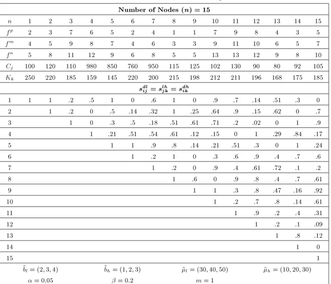
Let it be supposed that this example relates to health care services where the low-level servers provide primary services and the high-level servers provide high-level health care services. In this problem, there is a network with 15 nodes that represent dierent regions; estimation of the approximate demand rate for low-level services is given by ~fi= (fip; fim; fio). The
distance between two nodes is measured and treated in terms of the distance standard for low-level and high-level services and on the basis of such treatment, the degrees of membership are determined. In this problem, it is assumed that the distance standards are the same for low-level and high-level services, so that the membership degrees for the distance between nodes are identical for both low-level and high-level services, i.e., sdl
ij = slhjk= sdhik. The maximum allowable
number of customers is determined, approximately, for both levels and are assumed to be ~bl = (2; 3; 4) and
~bh= (1; 2; 3). The service rate at each level of servers
is determined by ~l= (30; 40; 50) and ~h= (10; 20; 30).
The percentage of low-level service demands, which are referred to the high-level centers, is = 0:2 for all demand nodes.
So, under these circumstances, one seeks to locate the servers and allocate the demand nodes to the servers in such a way that all demand nodes be covered by a predetermined minimum degree of membership with the minimum cost of locating the servers. To achieve this purpose, the branch and bound method is used to solve a small-scaled typical problem. The optimal solutions, obtained for the probabilistic model proposed by Marianov and Serra [1], as well as the fuzzy model are compared.
On the basis of the results obtained, a comparison of the probabilistic and fuzzied models is appropriate. Table 2 shows the optimal solution for the probabilistic HIQ-LSCP. In this problem, the low-level servers are located at nodes 1, 2 and 8 and the high-level servers are located at nodes 5 and 10. In the probabilistic version, demand node i, can be covered by the low-level server, j , and the high-low-level server, k, only when its distance from the servers is less than, or equal to, the distance standard. For example, demand node 6 is covered by low-level server 8. Therefore, in the probabilistic HIQ-LSCP, each demand node can be covered by just one server. So, one demand node cannot select a server from the available list of servers and must ask for service from the specied server designated for this purpose.
Table 1. Parameter values for the example. Number of Nodes (n) = 15
n 1 2 3 4 5 6 7 8 9 10 11 12 13 14 15
fp 2 3 7 6 5 2 4 1 1 7 9 8 4 3 5
fm 4 5 9 8 7 4 6 3 3 9 11 10 6 5 7
fo 5 8 11 12 9 6 8 5 5 13 13 12 9 8 10
Cj 100 120 110 980 850 760 950 115 125 102 130 90 80 92 105
Kk 250 220 185 159 145 220 200 215 198 212 211 196 168 175 185
sdl
ij = slhjk = sdhik
1 1 1 .2 .5 1 0 .6 1 0 .9 .7 .14 .51 .3 0
2 1 .2 0 .5 .14 .32 1 .25 .64 .9 .15 .62 0 .7
3 1 0 .3 .5 .18 .51 .61 .71 .2 .02 0 1 .9
4 1 .21 .51 .54 .61 .12 .15 0 1 .29 .84 .17
5 1 1 .9 .8 .14 .21 .51 .3 0 1 .24
6 1 .2 1 0 .3 .6 .9 .4 .7 .6
7 1 .2 0 .9 .4 .61 .72 .1 .2
8 1 .6 0 .9 .8 .4 .7 .61
9 1 1 .3 .8 .47 .16 .92
10 1 .2 .7 .8 .14 .61
11 1 .9 .2 .4 .31
12 1 .2 .1 .09
13 1 .8 .12
14 1 0
15 1
~bl= (2; 3; 4) ~bh= (1; 2; 3) ~l= (30; 40; 50) ~h= (10; 20; 30)
= 0:05 = 0:2 m = 1
Table 2. The optimum solution for the referral HIQ-LSCP. Low-Level Servers Location: 1, 2, 8
High-Level Servers Location: 5, 10
Demand Nodes Covered by the Low- and High-Level Servers (Xijk)
Low-Level Nodes
Servers 1 2 3 4 5 6 7 8 9 10 11 12 13 14 15
1 1 0 0 0 0 0 1 0 0 0 0 0 0 0 0
2 0 1 1 0 0 0 0 0 0 0 0 0 0 0 1
8 0 0 0 0 0 1 0 1 0 0 0 0 0 1 0
High-Level Servers
5 0 0 0 1 1 0 0 0 0 0 0 1 0 0 0
10 0 0 0 0 0 0 0 0 1 1 1 0 1 0 0
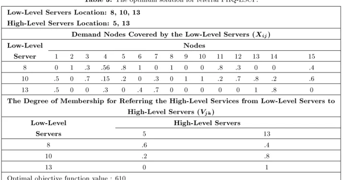
Table 3. The optimum solution for referral FHQ-LSCP. Low-Level Servers Location: 8, 10, 13
High-Level Servers Location: 5, 13
Demand Nodes Covered by the Low-Level Servers (Xij)
Low-Level Nodes
Server 1 2 3 4 5 6 7 8 9 10 11 12 13 14 15
8 0 1 .3 .56 .8 1 0 1 0 0 .8 .3 0 0 .4
10 .5 0 .7 .15 .2 0 .3 0 1 1 .2 .7 .8 .2 .6
13 .5 0 0 .3 0 .4 .7 0 0 0 0 0 1 .8 0
The Degree of Membership for Referring the High-Level Services from Low-Level Servers to High-Level Servers (Vjk)
Low-Level High-Level Servers
Servers 5 13
8 .6 .4
10 .2 .8
13 0 1
Optimal objective function value : 610
restrict each demand node to receive service from just one server. Besides, it does not seem real to deprive a demand node from receiving service, on the basis that its distance from a server is somewhat larger than the distance standard.
In the fuzzied hierarchical models that are de-veloped in this paper, each demand node can be covered by any low- or high-level server with a degree of membership. On the other hand, the models are equipped to consider priorities, in order to ask for and render services. In fact, in these models, each server provides service on the basis of its own priorities (degree of membership), in the same way that each demand node chooses to receive service from servers according to its own priorities. When the conditions of rendering service are identical for all servers, distance becomes the measure, on the basis of which a demand node assigns priorities to servers. In this way, each demand node prefers to go to its nearest server and if this server is occupied, to the next nearest server and so on.
In the FHQ-LSCP model, each demand node assigns a priority to each low- and high-level server on the basis of the degree of membership for its own distance from each server (sdl
ij, slhjk, sdhik). As Table 3
indicates, low-level servers for FHQ-LSCP are located at nodes 8, 10 and 13 and high-level servers are located at nodes 5 and 13. All of the demand nodes are covered by servers according to the degrees of membership. For example, the demand node 6 is covered by the low-level servers 8 and 13, with degrees of membership 1 and 0.8 and, for level services, is covered by the high-level servers 5 and 13, with the degrees of membership
0.6 and 1. This means that node 6 gives the highest priority to the low-level server 8 and less priority to the low-level server 13. The FHQ-LSCP model makes it possible for servers to assign their own priorities as well. This is accomplished by Xl
ij, and Xikh, which stand for
the degrees of membership for covering demand nodes. For instance, for the low-level server 8, demand nodes 1, 6 and 8 have the highest priority for receiving service, demand nodes 5 and 11 have the second highest priority and so on. As can be seen in Table 3, each demand node may be covered by various servers and there is a possibility that none of the demand nodes is deprived of receiving service. This obviously is the advantage of a fuzzy treatment of the problem.
CONCLUSIONS AND FUTURE EXTENSIONS
This work presents two new fuzzied queueing location set covering models for referral and nested hierarchical systems, which are code named referral FHQ-LSCP and nested FHQ-LSCP. The parameters of these mod-els are estimated approximately and are dened as fuzzy numbers. The constraints of service quality are also assumed to be fuzzy numbers. The allocation variables are assumed as the degrees of membership and the demand nodes can set their own priorities to select the appropriate server from a list, according to the degrees of membership. So, it seems that the models developed in this paper are closer to the real situation.
The nal models are transformed into mixed integer programming models. Since the LSCP model is
NP-Hard [19] and the derived 0-1 integer programming model in this paper can be reduced to the LSCP model in polynomial time, it is also NP-Hard. Heuristic methods can be developed for the solution of these problems as an extension. Other extensions include the developing of models for coherent LSCP fuzzy hierarchical queueing systems. It is also possible to develop similar models for the Maximal Covering Loca-tion Problem (MCLP), Maximal Availability LocaLoca-tion Problem (MALP) and other location models. Finally, the development of hierarchical models with more than two service levels can be investigated.
ACKNOWLEDGMENT
The authors are indebted to the anonymous reviewer whose constructive comments and suggestions have helped to enhance the quality of this article.
REFERENCES
1. Marianov, V. and Serra, D. \Hierarchical location-allocation models for congested systems", European Journal of Operational Research, 135, pp 195-205 (2001).
2. Toregas, C., Swain, R., ReVelle, C. and Bergman, L. \The location of emergency service facilities", Opera-tions Research, 19, pp 1363-1373 (1971).
3. Church, R.L. and Eaton, D.L. \Hierarchical location analysis using covering objectives", in Spatial Anal-ysis and Location-Allocation Models, Ghosh, A., and Rushton, G., Eds., New York, Van Nostrand Reinhold (1987).
4. Gerrard, R.A. and Church, R.L. \A generalized ap-proach to modeling the hierarchical maximal covering location problem with referral", Papers of the Regional Science Association, 73(4), pp 425-454 (1994). 5. Serra, D. and ReVelle, C. \The pq-median problem:
location and districting of hierarchical facilities", Lo-cation Science, 1, pp 299-312 (1993).
6. Serra, D. and ReVelle, C. \The pq-median problem: location and districting of hierarchical facilities-2. Heuristic solution methods", Location Science, 2, pp 63-82 (1994).
7. Serra, D., Marianov, V. and ReVelle, C. \The maxi-mum capture hierarchical problem", European Journal of Operational Research, 62(3), pp 363-371 (1992). 8. Serra, D. \The coherent covering location problem",
Papers in Regional Science: The Journal of RSAI, 75(1), pp 79-101 (1996).
9. Canos, M.J., Ivorra, C. and Liern, V. \Exact algorithm for the fuzzy p-median problem", European Journal of Operational Research, 116, pp 80-86 (1999).
10. Woodyatt, L.R., Stott, K.L., Wolf, F.E. and Vasko, F.J. \An application combining set covering and fuzzy sets to optimally assign metallurgical grades to cus-tomer orders", Fuzzy Sets and Systems, 53, pp 15-26 (1993).
11. Sahin, G. and Sural, H. \A review of hierarchical facility location models", Computers & Operations Research, 34, pp 2310-2331 (2007).
12. Shavandi, H. and Mahlooji, H. \Fuzzy queueing location-allocation models for congested systems", In-ternational Journal of Industrial Engineering, 11(4), pp 364-376 (2004).
13. Shavandi, H., Mahlooji, H., Eshghi, K. and Khanmo-hammadi, S. \A fuzzy coherent hierarchical location-allocation model for congested systems", Scientia Iran-ica, 13(1), pp 14-24 (2006).
14. Shavandi, H. and Mahlooji, H. \A fuzzy queueing max-imal covering location-allocation model with a genetic algorithm for congested systems", Applied Mathemat-ics and Computation, 181, pp 440-456 (2006). 15. Dubois, D. and Prade, H., Fuzzy Sets and Systems:
Theory and Applications, New York: Academic (1980). 16. Sugeno, M. \An introductory survey of fuzzy control",
Information Science, 36, pp 59-83 (1985).
17. Lee, C. \Fuzzy logic in control systems: fuzzy logic controller, parts 1 and 2", IEEE Transaction Systems, Man & Cybern, 20, pp 404-435 (1990).
18. Jo, J.B., Tsujimura, Y., Gen, M. and Yamazaki, G. \A delay model of queueing network systems based on fuzzy sets theory", Computers and Industrial Engi-neering, 25, pp 143-146 (1993).
19. Marianov, V. and ReVelle, C. \The queueing proba-bilistic location set covering problem and some exten-sions", Socio-Economic Planning Sciences, 28(30), pp 167-178 (1994).