This may be the author s version of a work that was submitted/accepted for publication in the following source:

(1)

This may be the author’s version of a work that was submitted/accepted

for publication in the following source:

Jacobson, Adam

,

Chen, Zetao

,

Rallabandi, Venkateswara

, &

Milford,

Michael

(2015)

Multi-scale place recognition with multi-scale sensing.

In Li, H & Kim, J (Eds.)

Proceedings of the Australasian Conference on

Robotics and Automation 2015.

Australian Robotics and Automation Association, Australia, pp. 1-10.

This file was downloaded from:

https://eprints.qut.edu.au/114371/

c

Copyright 2015 [please consult the author]

This work is covered by copyright. Unless the document is being made available under a Creative Commons Licence, you must assume that re-use is limited to personal use and that permission from the copyright owner must be obtained for all other uses. If the docu-ment is available under a Creative Commons License (or other specified license) then refer to the Licence for details of permitted re-use. It is a condition of access that users recog-nise and abide by the legal requirements associated with these rights. If you believe that this work infringes copyright please provide details by email to [email protected]

Notice

:

Please note that this document may not be the Version of Record

(i.e. published version) of the work. Author manuscript versions (as

Sub-mitted for peer review or as Accepted for publication after peer review) can

be identified by an absence of publisher branding and/or typeset

appear-ance. If there is any doubt, please refer to the published source.

(2)

Multi-Scale Place Recognition with Multi-Scale Sensing

Adam Jacobson, Zetao Chen, Venkateswara Rao Rallabandi and Michael Milford

∗

Abstract

Most robot navigation systems perform place recognition using a single sensor modality and using one, or at most two heterogeneous map scales. In contrast, mammals likely per-form navigation by combining sensing from a wide variety of modalities including vision, auditory, olfaction and tactile senses. Re-cent robotics research has shown that using multiple homogeneous mapping scales im-proves localization performance; but this re-search has used only a single visual sensing modality, missing out on the inherent vari-ation in spatial localizvari-ation specificity pro-vided by different sensors like cameras and WiFi. In this paper we develop a multi-scale, multi-sensor system for mapping and localization, that combines spatial localiza-tion hypotheses from different sensors and at different scales to calculate an overall lo-calization estimate. In two real-world exper-iments across a library and university cam-pus, we evaluate the place recognition per-formance of the proposed multi-scale sens-ing ussens-ing camera and WiFi sensory input. The results demonstrate that a universal im-provement in place recognition performance is achieved using the multi-scale system.

1 Introduction

In this work, we present a suite of sensor fusion al-gorithms designed to leverage multiple sensors with different levels of spatial acuity, evaluating the bene-fits of the techniques in multiple environments. In-spired by biological research into rodent mapping, it has been shown that rodents utilise a process of combining multiple maps of varying spatial resolu-tion [Hafting et al., 2005]. The maps are a collec-tion of neurons arranged in a grid pattern, where

∗_{A. Jacobson, Z. Chen, V. Rallabandi and M.}

Milford are with the School of Electrical

Engi-neering and Computer Science at the

Queens-land University of Technology, Brisbane, Australia,

[email protected]. This work was

supported by a funding from the Australian Research Council Centre of Excellence CE140100016 in Robotic Vision and a Future Fellowship FT140101229 to MM.

a1

a₄ a₃

a₂

a₅ a1 a2 a3 a4 a5

Camera Snapshots:

WiFi Snapshot:

a1 a2 a3 a4 a5 Camera Snapshots:

WiFi Snapshot:

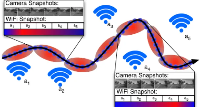
Figure 1: Illustration of multiple scale sensor fusion. Red ellipses represent the spatially sparse WiFi local-isation signal and the blue circles represent the spa-tially specific camera localisation results. The combi-nation of the two localisation results enables superior place localisation performance.

cells representing vertices “fire” when the rodent is in a particular location. The area represented by the grid cells in each layer can vary from a few cen-timetres to many meters [Burak and Fiete, 2009; Welinderet al., 2008]. The combination of these lay-ers is believed to enable robust navigation in a range of environments.

Previous work has investigated the use of mul-tiple maps for navigation, leveraging a local met-ric map and global topological map to improve the real-time performance of a robot [Bosse et al., 2003; Kuiperset al., 2004]. Previous research has also inves-tigated the potential impact of using multiple similar maps of different scales to improve robotic navigation systems [Chenet al., 2014], where maps were created by artificially segmenting image data from a single camera sensor into clusters of different sizes, learning a representation of space at different spatial levels.

In this paper, we focus on integrating commodity sensors, such as camera and WiFi sensors, which nat-urally produce localisation results of different spatial resolution, as seen in Fig. 1. We present a suite of sensor fusion techniques and provide an analysis into the benefits of utilising sensors with varying spatial resolution. We present an evaluation of each sen-sor fusion technique in two environments, including a highly aliased library environment and a campus environment, and use a Precision-Recall metric and

(3)

an Error-Recall metric to evaluate performance. The paper proceeds as follows. In Section 2, we re-view the robotic and biological mapping schemes with a focus on multi-scale representations of the world. Section 3 presents our approach describing in detail the place recognition system and the proposed multi scale sensor fusion techniques. In Section 4 we present the experimental setup, with the results of multiple levels of evaluation presented in Section 5. Section 6 discusses the outcome of the research and areas of future work.

2 Background

In this section, we review current research in the areas of Simultaneous Localization And Mapping (SLAM) [Dissanayake et al., 2001] with a focus on systems utilizing cameras or WiFi sensor modalities. We also review biological navigation processes with a focus on the entorhinal-hippocampal (EC) formation.

2.1 Simultaneous Localization And

Mapping

The focus of this work is to improve localisation capa-bilities by utilising sensors with different spatial res-olutions. Previous research investigated utilising a combination of local and global mapping techniques to improve navigation and compute capabilities. The Atlas system [Bosseet al., 2003] and the hybrid exten-sion to the Spatial Semantic Hierarchy [Kuiperset al., 2004; Kuipers and Byun, 1991] leverage local metric maps and global topological maps to achieve real-time navigation and map over large spaces.

Individually, cameras and WiFi have been used for localisation in many environments. Camera based lo-calisation systems use images taken within an envi-ronment to create unique identifiers of places. FAB-MAP [Cummins and Newman, 2011] leverages a cam-era to perform mapping over 1000km, other camcam-era- camera-only based systems have performed navigation utilis-ing a sole camera producutilis-ing impressive results

[Davi-son et al., 2007; Andreasson et al., 2008; Paz et al.,

2008; Konolige and Agrawal, 2008; Kawewong et al., 2010]. The images taken by a camera typically repre-sent a very specific location in the environment; de-pending on an environment, slight movement of the camera can produce very different images which re-sults in a mapping system which is very spatially specific. Images taken in the same location produce very strong matching scores however slight deviation in position can produce very weak matching scores. Feature-based approaches can alleviate this problem to some degree however introduces sensitivity to en-vironmental appearance change.

In contrast, depending on Wi-Fi infrastructure, the WiFi sensing modality produces a sparse localisa-tion signal, requiring large changes in pose to change matching scores. There are a number of techniques which leverage WiFi for localisation and mapping in-cluding Wi-Fi GraphSLAM [Huang et al., 2011] and the Distributed Particle Filter SLAM (DPSLAM) sys-tem [Faragher et al., 2012] and others [Weyn, 2011;

Ferriset al., 2007]. These techniques all utilise Wi-Fi fingerprinting, a process of sampling all available Wi-Fi devices and recording the MAC address and the associated signal strength for each device, producing a unique snapshot of an environment to enable local-isation. The broad spatial nature of the WiFi sensor prohibits it from achieving precise localisation results and limits its applications in a robotics domain.

Previous work investigated the combination of Wi-Fi and camera sensing modalities to combat the effect of day/night transitions [Berkvenset al., 2014], utilis-ing localisation results from each sensor in competitive nature. The work presented in this paper investigates the improvement of localisation capabilities using sen-sors of different spatial resolution.

2.2 Biological Multi-Scale Mapping

Genetically similar rats can be found all over the world, utilising the same neural machinery for map-ping and navigation to live and thrive in incredibly diverse and unique environments. This autonomy and the mapping capabilities displayed are a far cry from the current capabilities of modern robotic systems.

Biological research investigating the neuronal nav-igational processes in rats has identified a number of regions in the brain believed to be associated with performing mapping. The most recently discov-ered mapping neurons are the“grid” cells within the entorhinal-hippocampal formation and the medial en-torhinal cortex (MEC) [Hafting et al., 2005]. These regions leverage a grid-like representation of space to store spatial information, creating a high poten-tial (firing) whenever the rodent is located at a ver-tex of a grid. Even more interesting is the occur-rence of multiple layers of these grid-cells which en-code space at different scales, where grid vertices can represent areas from a few square centimetres to many square metres. It is this integrated mapping process which is believed to enable efficient mapping of ar-bitrarily large environments [Burak and Fiete, 2009; Welinderet al., 2008].

The benefit of multiple spatial scales for robotic ap-plications has been investigated in [Chenet al., 2014] utilising a single sensor. However, the work presented in [Chen et al., 2014] utilises sensory data which is artificially clustered to produce spatially diverse lo-calisation results. The work presented in this paper investigates the benefits of incorporating sensors with a natural spatial separation to improve robotic local-isation capabilities.

3 Approach

In this section, we describe the place recognition tech-niques used for the Wi-FI and camera sensor modal-ities. We also describe in detail our proposed sensor fusion techniques which leverage the varying spatial scales of each of the sensors.

(4)

3.1 Place Recognition

Camera

All images are converted to greyscale and are down-sampled to a a resolution of 48×64. We leverage the Sum of Absolute Difference (SAD) or L1_-norm

com-parison metric for evaluating images [Ballet al., 2013]. Using Equation 1, every new image,I, is compared to all previously captured images,Jj_{, producing a}

differ-ence score for each location in the environment. We account for small lateral shifts of the camera by shift-ing the query image (usshift-ing a shift range of ±ys and

±xs).

d(j) = argmin −xs<x<xs

−ys<y<ys

1

RxRy Rx X

u=0 Ry X

v=0

|I(u,v,x,y)−J₍j_u,v₎| (1)

where I(u,v,x,y) represents uth and vth pixels of the

current offset image, J₍j_u,v₎ is the uth _and _vth _pixels

of the jth_{database image.} _Rx _and_Ry _{are the x and}

y resolution of the images according to the offset per-formed. Each new image is added to the databaseJ

for later comparison to new samples.

WiFi Localisation

This work utilises the WiFi fingerprinting technique presented in [Weyn, 2011] for localisation. WiFi fin-gerprinting relies on local WiFi infrastructure to per-form localisation, each access point in range is queried and the received signal strength (RSS) from each de-vice is used as a unique identifier for localisation.

A fingerprintzis denoted as:

z={(s1, a1),(s2, a2), ...,(si, ai)} (2)

wheresiis the RSS value received from access point

ai.

New WiFi fingerprints are collected as the robot moves through an environment and compared to all previous WiFi fingerprints. Interestingly, unlike a camera or other sensor modalities, the available WiFi access points changes depending on location, environ-mental conditions and local infrastructure which al-lows for the implementation of rewards and penalties for fingerprints depending on the correlation to previ-ously stored fingerprints.

Comparison of each fingerprint requires determin-ing the similarity between access points which exist in both the query and database fingerprints, whit, and

evaluating the signal strength of access points which are missing from the query fingerprint, wmiss or are missing from the database fingerprint,wextra.

Each new fingerprint collected is compared to the

jth_{fingerprint using:}

whit(j) =

H−1 Y

x=0 e−

(sx−sjx)2

2σ2 ₍₃₎

wheresxandsjxare thexthaccess point of the current

and jth_{fingerprint, respectively.} _H _{is the number of}

RSSI (dBm)

Penalty

-120 -110 -100 -90 -80 -70 -60 -50 -40 -30 -20 0

0.1 0.2 0.3 0.4 0.5 0.6 0.7 0.8 0.9 1

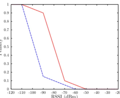
Figure 2: This figure shows the conversion from a RSS value to a penalty for missing access points (red solid line), and extra access points (blue dashed line). matching access points. The penalties for missing or extra access points are calculated using:

wextra(j) =

E−1 Y

x=0 e−

(Pextra(sx))2

2σ2 ₍₄₎

wmiss(j) =

M−1

Y x=0

e−

(Pmiss(sj x))2

2σ2 ₍₅₎

where the penaltiesPextraandPmiss calculated using the function shown in Fig. 2. E andM represent the number of extra access points in the current finger-print and the number of missing access points from thejthfingerprint, respectively. σ2is set to 20 dBm2, based on research by [Chiouet al., 2009].

The final matching scorew(j) is calculated using:

w(j) = Hp

whit(j)×wextra(j)×wmiss(j)× H

H+E+M

(6)

3.2 Multi-Scale Sensory Fusion

There are multiple ways to combine sensory data for place recognition. Here, we present four methods for evaluations from here denoted as Techniques 1-4.

Technique 1: Super Template Sensor Weighting

Technique 1 involves combining sensor modalities into weighted “super templates”. Due to the different cap-ture rates of each sensor (WiFi=1Hz, Camera=3Hz), the difference scores of the WiFi sensor are linearly interpolated to match the sampling rate of the cam-era sensor. Once the WiFi data is interpolated, the difference scores from each sensor are weighted and combined according to:

C(j) =k×d(j) + (k−1)× −w′₍

j) (7)

where C(j) is the current super template difference score, d(j) and w′₍_j_{) is the} _jt_h_{camera and}

interpo-lated WiFi difference scores. k represents the sensor weights and has a value of k ∈ ℜ+≤1. To account for

the fact that for WiFi, a good WiFi match score is a maximum, we transformed the match scores to enable searching for a minimum match score, as is done with

(5)

0m 1m5m Start

End

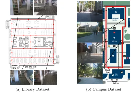
(a) Library Dataset

Start End

0 30 60 120

Metres (b) Campus Dataset

Figure 3: Datasets used for Sensor Fusion Evaluation. the camera sensor, by multiplying the matching score

by−1.

In previous works, the sensor weights have been de-termined by online sensor evaluation techniques [Ja-cobson et al., 2015; Milford and Jacobson, 2013], in this work it is manually selected to investigate the impact of each sensor to the place recognition system.

Technique 2: Spatial Dilation

Technique 2 dilates the spatial resolution of the WiFi sensor using a Gaussian kernel. We dilate the spatial resolution of the linearly interpolated WiFi matching scores using a 2D Gaussian kernel with a kernel size of

Kand a standard deviation ofσ, as seen in Fig. 4. We select a range of K and σvalues to simulate varying spatial resolutions. The difference scores from each sensor is then combined according to:

C(j) =d(j) +−w′

b(j) (8)

wherew′

b(j) is the Gaussian blurred interpolated WiFi

matching scores.

Technique 3: Voting

Technique 3 works on the premise that a place match is more likely to be correct if multiple sensors agree that a hypothesis is correct. To facilitate this, the

S best place hypothesis are selected from each sensor based on each sensors matching scores. Each hypoth-esis is compared against each of the other hypothhypoth-esis; if the hypotheses align, the difference score for that location is set toC(j) =d(j) +−w(j), otherwise the match is ignored. This enables an incorrect place hy-pothesis which may have the best matching score to be filtered out.

Technique 4: Gaussian Combination

Technique 4 converts camera differences scores using a Gaussian kernel which is then multiplied with the interpolated WiFi matching scores as seen:

C(j) =−e−(d(2jσ)−2X)2 ×w′(j) (9)

w' w

b'

Figure 4: Example of the spatial dilation of the WiFi sensor using a 2D Gaussian Kernel. The difference score matrix is a collection of difference scores mea-sured during the course of the experiment, Y-axis rep-resents database frames and they X-axis reprep-resents the query dataset collected during the experiment. The variables X and σ alter what is considered a “good” match for the camera sensor.

Selecting a Place Match

To determine if a location is a place match, the place hypothesis with the smallest matching score is found using:

b= argmin

0≤j<n−γ

C(j) (10)

where n is the number of sensory snapshots stored within the database andγis a recency threshold.

The current best matching sensory snapshot is de-termined to be a place match if the difference score is below a global matching thresholdsthresh:

m=

1, C(b)≤sthresh

0, C(b)> sthresh (11)

It is this threshold,sthresh, which determines if a

par-ticular location is a loop closure. sthresh is tuned to

(6)

Figure 5: Dataset acquisition tools include a standard laptop with WiFi enabled and an external webcamera.

4 Experimental Setup

In this section, we describe the hardware used for data acquisition, testing environment and system parame-ters.

4.1 Testing Environments and Dataset

Acquisition

In this work, datasets from two environments are used to evaluate the sensor fusion technique. The first dataset, the Library dataset, involves walking a path throughout a floor of the library building with multi-ple repeats at the Queensland University of Technol-ogy Gardens Point campus, seen in Fig. 3a. The en-vironment has a number of open areas, corridors and suffers from a large amount of perceptual aliasing.

The second dataset, the Campus dataset, consists of walking two laps around the Queensland University of Technology Gardens Point campus, seen in Fig. 3b. The dataset has a collection of natural scenery, build-ings and pedestrian traffic.

The dataset acquisition device for the Library and Campus datasets consist of a standard laptop capable of capturing WiFi information and an external web-camera, seen in Fig. 5a.

We also provide a small scale experiment, allowing a visualisation of the different spatial scales of the WiFi and camera sensors. A robot is placed in three loca-tions where it captures a single WiFi fingerprint and image, the robot is then moved forward continually acquiring data and measuring the distance from the first sample. The collected data is compared to the first sample to illustrate the spatial resolution of each sensor. This experiment was performed in an office environment similar to the Library dataset.

4.2 System Parameters

The system parameters utilized for this work were set to a constant value for all experiments and can be found in Table 1 and Table 2.

Table 1: Experimentation System Parameters Parameter Campus Library

γ 30s 30s

Ground Truth 10m 10m

4.3 System Evaluation

We utilise a Precision-Recall metric and Error-Recall metric for evaluating the sensor fusion techniques in each of the datasets. We compare each system us-ing ground truth maps and consider place matches

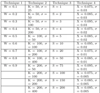
Table 2: Sensor Fusion Technique Parameters

Technique 1 Technique 2 Technique 3 Technique 4

W = 0.1 K = 50,σ=

25

S = 1 X = 0.075,σ

= 0.03

W = 0.2 K = 50,σ=

50

S = 2 X = 0.085,σ

= 0.03

W = 0.3 K = 50,σ=

100

S = 3 X = 0.095,σ

= 0.03

W = 0.4 K = 50,σ=

200

S = 4 X = 0.075,σ

= 0.02

W = 0.5 K = 100,σ

= 50

S = 5 X = 0.085,σ

= 0.02

W = 0.6 K = 100,σ

= 100

S = 10 X = 0.095,σ

= 0.02

W = 0.7 K = 100,σ

= 200

S = 20 X = 0.075,σ

= 0.01

W = 0.8 K = 100,σ

= 400

S = 50 X = 0.085,σ

= 0.01

W = 0.9 K = 200,σ

= 50

S = 75 X = 0.095,σ

= 0.01

K = 200,σ

= 100

S = 100 X = 0.075,σ

= 0.005

K = 200,σ

= 200

S = 150 X = 0.085,σ

= 0.005

K = 200,σ

= 400

S = 200 X = 0.095,σ

= 0.005

within the ground truth thresholds, seen in Table 1, as true positives. We utilise the Error-Recall metric as it enables an analysis of the relative performance improvement for each sensor fusion technique.

Ground truth maps for the Library and Campus datasets consists of manually labelling frame corre-spondences between each traverse.

5 Results

Here, we present the results for multiple multi-scale sensor fusion techniques.

5.1 Multi Sensor Fusion Evaluations

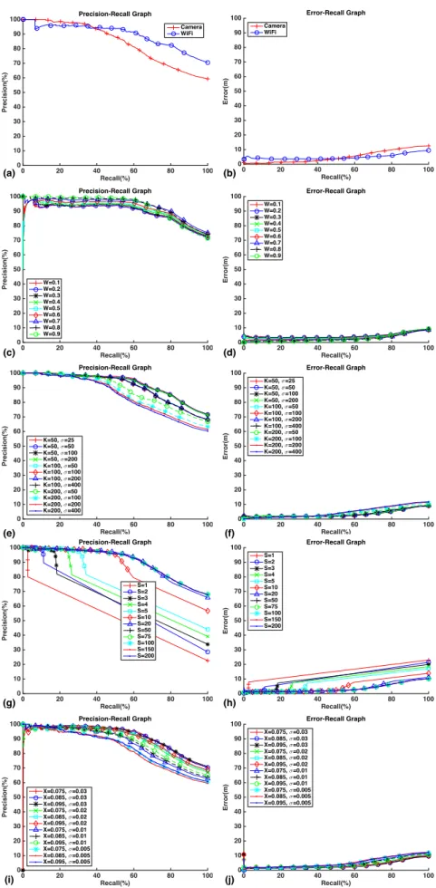
For each sensor fusion technique, we evaluate multiple parameters seen in Table 2. The results for Library dataset can be seen in Fig. 8 with the raw performance of Camera and WiFi sensors producing 12.32% and 6.57% Recall at 100% Precision, as seen in Table 3. It can be seen in Fig. 8(d, f and j) that the Error-Recall graphs for Techniques 1,2 and 4 are superior to the in-dividual sensor Error-Recall performance in Fig. 8(b). It can also be seen that the Error-Recall graph for Technique 3 (Fig. 8(h)) improves upon individual sen-sor results when S ={10,20,50,75,100,150,200}. Tech-niques 1 and 2 improved absolute precision results over a single sensor, achieving 15.13% and 18.34% re-call at 100% precision. The resulting Precision-Rere-call graphs created using Technique 1 and 2 are also supe-rior to that of either individual sensor and Technique 3 generates a result which is superior to the raw WiFi result, as seen in Fig. 6.

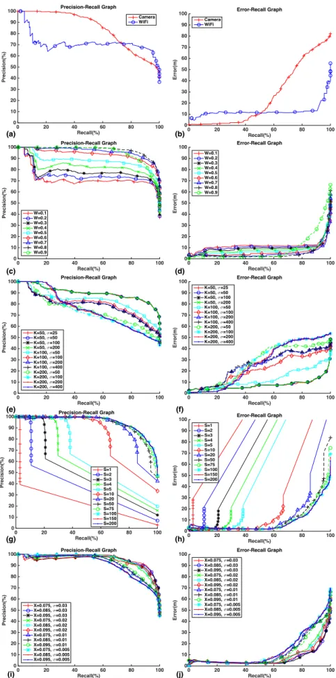
For the Campus Dataset, the Camera and WiFi produce 16.40% and 4.71% Recall at 100% Precision (Table 3). Fig. 7 show that all the sensor fusion techniques are capable of improving the performance above what is capable with a single sensor modal-ity. The results in Fig. 9 show that all parameters for Techniques 1 and 4 (Fig. 9(d,j)) produce improved Error-Recall plots than WiFi alone. It can also be seen that all sensor fusion techniques have the poten-tial for improving the Error Recall graph. Techniques

(7)

Recall(%)

0 20 40 60 80 100

Precision(%)

0 10 20 30 40 50 60 70 80 90

100 Precision-Recall Graph

Camera WiFi T1: W=0.9 T2: K=50, σ=25 T3: S=2 T4: X=0.075, σ=0.02

Figure 6: Precision-Recall Graphs for the individual camera and WiFi sensor and the best results from Techniques 1-4 for the Library Dataset.

Recall(%)

0 20 40 60 80 100

Precision(%)

0 10 20 30 40 50 60 70 80 90

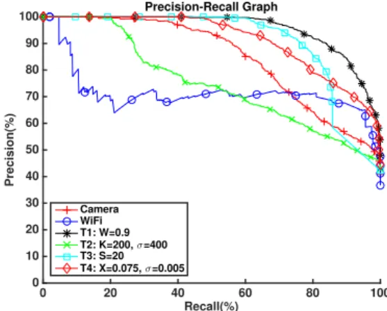
Camera WiFi T1: W=0.9 T2: K=200, σ=400 T3: S=20 T4: X=0.075, σ=0.005

Figure 7: Precision-Recall Graphs for the individual camera and WiFi sensor and the best results from Techniques 1-4 for the Campus Dataset.

1, 2, 3 and 4 (Fig. 9(c,e,g,i)) produce Precision-Recall results superior to WiFi or camera alone, achieving 44.3%, 17.53%, 54.45% and 42.55% Recall at 100% Precision. Technique 3 does not improve performance above either individual sensors forS ={1,2,3,4,5,}, however does significantly improve above a naive sen-sor implementation for all other tested parameters.

Evaluating the results from both datasets, it can be seen that Technique 1 (W = 0.9) consistently pro-duces a superior localisation result when compared to other sensors and parameters. The technique most sensitive to parameter selection is Technique 3, as il-lustrated by the Error-Recall plots in Fig. 8(h) and Fig. 9(h).

5.2 Example Place Matches

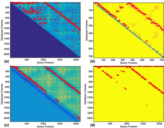
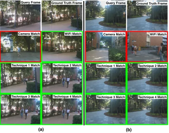
We present the difference score matrices for the Cam-era (Fig. 11(a)), WiFi (Fig. 11(b)) and Technique 2-3 (Fig. 11(c,d)). The sensor fusion techniques remove false positives generated by the camera sensor and in-creases the spatial resolution of the WiFi sensor which is evident from analysis of the second half of each of the difference score matrices which corresponds to the second lap of the environment.

Fig. 11 illustrates the capability of the sensor fu-sion methods to remove false positives of one (Fig. 11

Table 3: Maximum Recall at 100% Precision Fusion Methods which do not achieve 100%

Precision are denoted by “0.00”.

Fusion Method Library Campus

Camera 12.32 16.40

WiFi 6.56 4.71

Technique 1:W = 0.1 0.12 4.03

Technique 1:W = 0.2 0.12 4.59

Technique 1:W = 0.3 0.12 4.78

Technique 1:W = 0.4 0.06 7.78

Technique 1:W = 0.5 0.06 10.12

Technique Technique 1: W= 0.6

0.29 11.34

Technique 1:W = 0.7 1.11 12.37

Technique 1:W = 0.8 3.91 13.31

Technique 1:W = 0.9 15.13 44.33

Technique 2: K =

50, σ= 25

18.34 9.00

Technique 2: K =

50, σ= 50

15.07 9.47

Technique 2: K =

50, σ= 100

14.95 9.75

Technique 2: K =

50, σ= 200

14.95 9.75

Technique 2: K =

100, σ= 50

14.08 7.12

Technique 2: K =

100, σ= 100

13.61 6.37

Technique 2: K =

100, σ= 200

13.43 6.37

Technique 2: K =

100, σ= 400

13.43 6.37

Technique 2: K =

200, σ= 50

17.82 9.56

Technique 2: K =

200, σ= 100

7.07 16.03

Technique 2: K =

200, σ= 200

9.99 17.24

Technique 2: K =

200, σ= 400

9.29 17.53

Technique 3:S= 1 2.57 2.81

Technique 3:S= 2 7.89 9.93

Technique 3:S= 3 2.86 17.71

Technique 3:S= 4 3.33 23.81

Technique 3:S= 5 4.09 30.18

Technique 3:S= 10 5.72 44.89

Technique 3:S= 20 6.02 54.45

Technique 3:S= 50 6.02 6.28

Technique 3:S= 75 6.02 6.28

Technique 3:S= 100 6.02 6.28

Technique 3:S= 150 6.02 6.28

Technique 3:S= 200 6.02 6.28

Technique 4: X =

0.075, σ= 0.03

3.33 7.69

Technique 4: X =

0.085, σ= 0.03

0.93 7.59

Technique 4: X =

0.095, σ= 0.03

0.00 7.40

Technique 4: X =

0.075, σ= 0.02

4.67 6.94

Technique 4: X =

0.085, σ= 0.02

1.99 6.65

Technique 4: X =

0.095, σ= 0.02

0.00 7.22

Technique 4: X =

0.075, σ= 0.01

3.56 7.78

Technique 4: X =

0.085, σ= 0.01

1.11 4.78

Technique 4: X =

0.095, σ= 0.01

0.29 5.90

Technique 4: X =

0.075, σ= 0.005

3.15 42.55

Technique 4: X =

0.085, σ= 0.005

1.40 3.47

Technique 4: X =

0.095, σ= 0.005

1.75 4.22

(a)) or both (Fig. 11(b)) of the sensors. In both cases, all four sensor fusion techniques improve performance and filter out the false positives of the individual sen-sors.

(8)

Recall(%)

0 20 40 60 80 100

Precision(%) 0 10 20 30 40 50 60 70 80 90

Camera WiFi

Recall(%)

0 20 40 60 80 100

Precision(%) 0 10 20 30 40 50 60 70 80 90

W=0.1 W=0.2 W=0.3 W=0.4 W=0.5 W=0.6 W=0.7 W=0.8 W=0.9 Recall(%)

0 20 40 60 80 100

Precision(%) 0 10 20 30 40 50 60 70 80 90

K=50, σ=25 K=50, σ=50 K=50, σ=100 K=50, σ=200 K=100, σ=50 K=100, σ=100 K=100, σ=200 K=100, σ=400 K=200, σ=50 K=200, σ=100 K=200, σ=200 K=200, σ=400 Recall(%)

0 20 40 60 80 100

Precision(%) 0 10 20 30 40 50 60 70 80 90

S=1 S=2 S=3 S=4 S=5 S=10 S=20 S=50 S=75 S=100 S=150 S=200 Recall(%)

0 20 40 60 80 100

Precision(%) 0 10 20 30 40 50 60 70 80 90

X=0.075, σ=0.03 X=0.085, σ=0.03 X=0.095, σ=0.03 X=0.075, σ=0.02 X=0.085, σ=0.02 X=0.095, σ=0.02 X=0.075, σ=0.01 X=0.085, σ=0.01 X=0.095, σ=0.01 X=0.075, σ=0.005 X=0.085, σ=0.005 X=0.095, σ=0.005 Recall(%)

0 20 40 60 80 100

Error(m) 0 10 20 30 40 50 60 70 80 90

100 Error-Recall Graph

Camera WiFi

Recall(%)

0 20 40 60 80 100

Error(m) 0 10 20 30 40 50 60 70 80 90

0 20 40 60 80 100

Error(m) 0 10 20 30 40 50 60 70 80 90

K=50, σ=25 K=50, σ=50 K=50, σ=100 K=50, σ=200 K=100, σ=50 K=100, σ=100 K=100, σ=200 K=100, σ=400 K=200, σ=50 K=200, σ=100 K=200, σ=200 K=200, σ=400

Recall(%)

0 20 40 60 80 100

Error(m) 0 10 20 30 40 50 60 70 80 90

0 20 40 60 80 100

Error(m) 0 10 20 30 40 50 60 70 80 90

X=0.075, σ=0.03 X=0.085, σ=0.03 X=0.095, σ=0.03 X=0.075, σ=0.02 X=0.085, σ=0.02 X=0.095, σ=0.02 X=0.075, σ=0.01 X=0.085, σ=0.01 X=0.095, σ=0.01 X=0.075, σ=0.005 X=0.085, σ=0.005 X=0.095, σ=0.005 (a) (b) (c) (d) (e) (f) (g) (h) (i) (j)

Figure 8: Library Dataset Results. Single sensor Recall(a) and Error-Recall(b) graphs. The Precision-Recall and Error-Precision-Recall graphs for Technique 1 (c-d), Technique 2 (e-f), Technique 3 (g-h) and Technique 4 (i-j) are also presented.

(9)

Recall(%)

0 20 40 60 80 100

Precision(%) 0 10 20 30 40 50 60 70 80 90

X=0.075, σ=0.03 X=0.085, σ=0.03 X=0.095, σ=0.03 X=0.075, σ=0.02 X=0.085, σ=0.02 X=0.095, σ=0.02 X=0.075, σ=0.01 X=0.085, σ=0.01 X=0.095, σ=0.01 X=0.075, σ=0.005 X=0.085, σ=0.005 X=0.095, σ=0.005

Recall(%)

0 20 40 60 80 100

Precision(%) 0 10 20 30 40 50 60 70 80 90

0 20 40 60 80 100

Precision(%) 0 10 20 30 40 50 60 70 80 90

K=50, σ=25 K=50, σ=50 K=50, σ=100 K=50, σ=200 K=100, σ=50 K=100, σ=100 K=100, σ=200 K=100, σ=400 K=200, σ=50 K=200, σ=100 K=200, σ=200 K=200, σ=400 Recall(%)

0 20 40 60 80 100

Precision(%) 0 10 20 30 40 50 60 70 80 90

0 20 40 60 80 100

Precision(%) 0 10 20 30 40 50 60 70 80 90

Camera WiFi

Recall(%)

0 20 40 60 80 100

Error(m) 0 10 20 30 40 50 60 70 80 90

100 Error-Recall Graph S=1 S=2 S=3 S=4 S=5 S=10 S=20 S=50 S=75 S=100 S=150 S=200 Recall(%)

0 20 40 60 80 100

Error(m) 0 10 20 30 40 50 60 70 80 90

K=50, σ=25 K=50, σ=50 K=50, σ=100 K=50, σ=200 K=100, σ=50 K=100, σ=100 K=100, σ=200 K=100, σ=400 K=200, σ=50 K=200, σ=100 K=200, σ=200 K=200, σ=400 Recall(%)

0 20 40 60 80 100

Error(m) 0 10 20 30 40 50 60 70 80 90

X=0.075, σ=0.03 X=0.085, σ=0.03 X=0.095, σ=0.03 X=0.075, σ=0.02 X=0.085, σ=0.02 X=0.095, σ=0.02 X=0.075, σ=0.01 X=0.085, σ=0.01 X=0.095, σ=0.01 X=0.075, σ=0.005 X=0.085, σ=0.005 X=0.095, σ=0.005

Recall(%)

0 20 40 60 80 100

Error(m) 0 10 20 30 40 50 60 70 80 90

0 20 40 60 80 100

Error(m) 0 10 20 30 40 50 60 70 80 90

Camera WiFi (a) (b) (c) (d) (e) (f) (g) (h) (i) (j)

Figure 9: Campus Dataset Results. Single sensor Recall(a) and Error-Recall(b) graphs. The Precision-Recall and Error-Precision-Recall graphs for Technique 1 (c-d), Technique 2 (e-f), Technique 3 (g-h) and Technique 4 (i-j) are also presented.

(10)

Query Frames

500 1000 1500 2000

Database Frames

200 400 600 800 1000 1200 1400 1600 1800 2000

Query Frames

500 1000 1500 2000

Database Frames

200 400 600 800 1000 1200 1400 1600 1800 2000 Query Frames

500 1000 1500 2000

Database Frames

200 400 600 800 1000 1200 1400 1600 1800 2000

Query Frames

100 200 300 400 500 600 700

Database Frames

100

200

300

400

500

600

700

(a)

(c)

(b)

(d)

Figure 10: Example Difference Score Matrices for the Camera (a), WiFi (b), Technique 2 (c) and Technique (3). The Y axis represents learnt database frames, the X-axis represents the query frames. The red crosses denote the best matching difference score for each query frame.

5.3 Small Scale Experiment

The Small Scale Experiment is presented to demon-strate the different spatial scales of each of the sensors. Each experiment involved placing a robot in an envi-ronment and capturing data as the robot was moved forward, comparing each new sample to the first sam-ple collected. The results, seen in Fig. 12, illustrates how the camera matching score rapidly changes dur-ing the first 0.1m of the experiment, then remains constant. However, the WiFi matching scores, ex-cluding deviations due to sample noise, remains fairly constant over the whole 2m experiment.

6 Discussion and Future Work

This paper presented four different sensor fusion tech-niques to take advantage of the sensors with varying spatial acuity and investigate the robotic implications of biological research into rodent navigation, specifi-cally grid cells. We presented an analysis of each of the sensor fusion techniques in two environments demon-strating an improvement to absolute performance and relative mapping accuracy.

Future work will continue to investigate the ben-efits of biologically inspired multi scale implementa-tions, investigating benefits of other sensing modali-ties, leveraging sensor like radar or sonar which are spatially broad. Furthermore, we will investigate the impact of adding more than two sensory modalities, reviewing the upper limit of the performance gain from a multi-scale implementation.

References

[Andreassonet al., 2008] H Andreasson, T Duckett, and A Lilien-thal. A minimalistic approach to appearance-based visual slam. IEEE Transactions on Robotics, 24(5):1–11, 2008.

[Ballet al., 2013] David Ball, Scott Heath, Janet Wiles, Gordon Wyeth, Peter Corke, and Michael Milford. OpenRatSLAM: an

open source brain-based SLAM system. Autonomous Robots,

pages 1–28, 2013.

[Berkvenset al., 2014] Rafael Berkvens, Adam Jacobson, Michael Milford, Herbert Peremans, and Maarten Weyn. Biologically inspired slam using wi-fi. In Intelligent Robots and Systems. IEEE, 2014.

[Bosseet al., 2003] M Bosse, P Newman, J Leonard, M Soika, W Feiten, and S Teller. An atlas framework for scalable mapping. InInternational Conference on Robotics and Automation, vol-ume 2, pages 1899–1906, Taipei, Taiwan, 2003. IEEE.

[Burak and Fiete, 2009] Yoram Burak and Ila R Fiete. Accurate path integration in continuous attractor network models of grid cells.PLoS Comput Biol, 5(2):e1000291, 2009.

[Chenet al., 2014] Zetao Chen, Adam Jacobson, Ugur M. Erdem, Michael E. Hasselmo, and Michael Milford. Multi-scale bio-inspired place recognition. In 2014 IEEE International Con-ference on Robotics and Automation (ICRA), June 2014. [Chiouet al., 2009] Yih-Shyh Chiou, Chin-Liang Wang,

Sheng-Cheng Yeh, and Ming-Yang Su. Design of an adaptive posi-tioning system based on WiFi radio signals.Computer Commu-nications, 32(7-10):1245–1254, May 2009.

[Cummins and Newman, 2011] Mark Cummins and Paul Newman. Appearance-only slam at large scale with fab-map 2.0. The In-ternational Journal of Robotics Research, 2011.

[Davisonet al., 2007] Andrew J. Davison, Ian D. Reid, Nicholas D. Molton, and Olivier Stasse. Monoslam: Real-time single camera

slam. IEEE Transactions on Pattern Analysis and Machine

Intelligence, 29(6):1052–1067, 2007.

[Dissanayakeet al., 2001] G. Dissanayake, P.M. Newman,

S. Clark, H. Durrant-Whyte, and M. Csorba. A solution

to the simultaneous localisation and map building (slam)

problem. IEEE Transactions on Robotics and Automation,

2001.

[Faragheret al., 2012] R. M. Faragher, C. Sarno, and M. Newman. Opportunistic radio SLAM for indoor navigation using smart-phone sensors. InPosition Location and Navigation Symposium

(11)

Query Frame Ground Truth Frame

Camera Match WiFi Match

Technique 1 Match

Technique 3 Match Technique 4 Match

Query Frame Ground Truth Frame

Camera Match WiFi Match

Technique 3 Match Technique 4 Match

(b) (a)

Figure 11: Example place matches for the Campus dataset. All four sensor fusion techniques are capable of correcting a single sensor false place match (a) and when both sensors report false place matches (b)

m

0 0.2 0.4 0.6 0.8 1

Difference Score

0 0.2 0.4 0.6 0.8

1 Difference Score vs Distance

Camera WiFi

(a) Location 1

m

0 0.2 0.4 0.6 0.8 1

0 0.2 0.4 0.6 0.8

1 Difference Score vs Distance

Camera WiFi

(b) Location 2

m

0 0.2 0.4 0.6 0.8 1

Difference Score vs Distance

Camera WiFi

(c) Location 3

Figure 12: Illustration of the matching scores for WiFi and Camera sensors vs Distance in a number of dif-ferent environments

(PLANS), 2012 IEEE/ION, pages 120–128, Myrtle Beach, SC, April 2012. IEEE.

[Ferriset al., 2007] Brian Ferris, Dieter Fox, and Neil Lawrence. WiFi-SLAM using Gaussian process latent variable models. Pro-ceedings of the 20th International Joint Conference on Artifi-cial Intelligence, pages 2480–2485, 2007.

[Haftinget al., 2005] Torkel Hafting, Marianne Fyhn, Sturla Molden, May-Britt Moser, and Edvard I Moser. Microstructure of a spatial map in the entorhinal cortex.Nature, 436(7052):801– 806, 2005.

[Huanget al., 2011] Joseph Huang, David Millman, Morgan

Quigley, David Stavens, Sebastian Thrun, and Alok Aggarwal. Efficient, generalized indoor WiFi GraphSLAM. InInternational Conference on Robotics and Automation, 2011.

[Jacobsonet al., 2015] Adam Jacobson, Zetao Chen, and Michael Milford. Autonomous multisensor calibration and closed-loop fusion for slam.Journal of Field Robotics, 2015.

[Kawewonget al., 2010] A. Kawewong, N. Tongprasit, S. Tangru-amsub, and O. Hasegawa. Online and incremental appearance-based slam in highly dynamic environments. The International Journal of Robotics Research, 2010.

[Konolige and Agrawal, 2008] K. Konolige and M. Agrawal.

Frameslam: From bundle adjustment to real-time visual map-ping.IEEE Transactions on Robotics, 2008.

[Kuipers and Byun, 1991] B Kuipers and Y T Byun. A Robot Ex-ploration and Mapping Strategy Based on a Semantic Hierarchy of Spatial Representations.Robotics and Autonomous Systems, 8(1):47–63, 1991.

[Kuiperset al., 2004] Benjamin Kuipers, Joseph Modayil, Patrick Beeson, Matt MacMahon, and Francesco Savelli. Local Metri-cal and Global TopologiMetri-cal Maps in the Hybrid Spatial Semantic Hierarchy. InInternational Conference on Robotics and Au-tomation, New Orleans, USA, 2004.

[Milford and Jacobson, 2013] M Milford and A Jacobson. Brain-inspired Sensor Fusion for Navigating Robots. InInternational Conference on Robotics and Automation, Karlsruhe, Germany, 2013. IEEE.

[Pazet al., 2008] Lina M. Paz, Pedro Pinies, Juan D. Tardos, and Jose Neira. Large-scale 6-dof slam with stereo-in-hand. IEEE Transactions on Robotics, 2008.

[Welinderet al., 2008] Peter E Welinder, Yoram Burak, and Ila R Fiete. Grid cells: the position code, neural network models of ac-tivity, and the problem of learning. Hippocampus, 18(12):1283– 1300, 2008.

[Weyn, 2011] Maarten Weyn. Opportunistic Seamless Localiza-tion. Phd thesis, Universiteit Antwerpen, 2011.