Review on application and comparison of metaheuristic techniques to multi-area economic dispatch problem

R E V I E W

Open Access

Review on application and comparison of

metaheuristic techniques to multi-area

economic dispatch problem

Jagat Kishore Pattanaik

, Mousumi Basu

and Deba Prasad Dash

Abstract

This paper presents both application and comparison of the metaheuristic techniques to multi-area economic dispatch (MAED) problem with tie line constraints considering transmission losses, multiple fuels, valve-point loading and prohibited operating zones. The metaheuristic techniques such as differential evolution, evolutionary programming, genetic algorithm and simulated annealing are applied to solve MAED problem. These metaheuristic techniques for MAED problem are evaluated on three different test systems, both small and large, involving varying degree of complexity and the results are compared against each other.

Keywords: Multi-area economic dispatch, Tie line constraints, Differential evolution, Evolutionary programming, Genetic algorithm, Simulated annealing

1 Introduction

Economic dispatch (ED) is one of the important optimization problems in power system operation. ED allocates the load demand among the committed genera-tors most economically while satisfying the physical and operational constraints in a single area. Generally, the generators are divided into several generation areas interconnected by tie-lines. Multi-area economic dispatch (MAED) is an extension of economic dispatch. MAED

determines the generation level and interchange

power between areas such that total fuel cost in all areas is minimized while satisfying power balance constraints, generating limits constraints and tie-line capacity constraints.

The economic dispatch problem is frequently solved without considering transmission constraints. However, some researchers have taken transmission capacity constraints into account. Shoults et al. [1] solved economic dispatch problem considering import and export constraints between areas. This study provides a complete formulation of multi-area generation sched-uling, and a framework for multi-area studies. Romano

et al. [2] presented the Dantzig–Wolfe decomposition

principle to the constrained economic dispatch of multi-area systems. An application of linear program-ming to transmission constrained production cost ana-lysis was proposed in Ref. [3]. Helmick et al. [4] solved multi-area economic dispatch with area control error. Wang and Shahidehpour [5] proposed a decomposition approach for solving multi-area generation scheduling with tie-line constraints using expert systems. Network flow models for solving the multi-area economic dispatch problem with transmission constraints have been pro-posed by Streiffert [6]. An algorithm for multi-area eco-nomic dispatch and calculation of short range margin cost based prices has been presented by Wernerus and Soder [7], where the multi-area economic dispatch problem was solved via Newton–Raphson’s method. Yalcinoz and Short [8] solved multi-area economic dispatch problems by using Hopfield neural network approach. Jayabarathi et al. [9] solved multi-area economic dispatch problems with tie line constraints using evolutionary programming. The dir-ect search method for solving economic dispatch problem considering transmission capacity constraints was pre-sented in Ref. [10]. Chen [11] develops a hybrid approach of combining sequential dispatch with a direct search method to deal with the multi-product and multi-area

* Correspondence:[email protected]

1_{Department of Power Engineering, Jadavpur University, Salt Lake City,}

Kolkata 700098, India

Full list of author information is available at the end of the article

electricity market dispatch problem. But these methods did not consider transmission loss.

With the emergence of metaheuristic techniques, attention has been gradually shifted to applications of such technology-based approaches to handle the complexity in-volved in real world problems. Metaheuristic techniques have been given much attention by many researchers due their ability to seek for the near global optimal solution.

This paper investigates the applicability of the following four metaheuristic techniques in the MAED problem: dif-ferential evolution (DE), evolutionary programming (EP), genetic algorithm (GA), and simulated annealing (SA).

Here, three types of MAED problems have been considered. These are A) multi area economic dispatch with quadratic cost function prohibited operating zones and trans-mission losses (MAEDQCPOZTL) B) multi area economic dispatch with valve point loading (MAEDVPL) C) multi area economic dispatch with valve point loading multiple fuel sources and transmission losses (MAEDVPLMFTL).

The metaheuristic techniques are evaluated against three different test systems for comparison with each other.

2 Problem formulation

The objective of MAED is to minimize the total cost of supplying loads to all areas while satisfying power balance constraints, generating limits constraints and tie-line capacity constraints.

Three different types of MAED problems have been considered.

2.1 MAEDQCPOZTL

The objective functionFt, total cost of committed

gener-ators of all areas, of MAED problem may be written as

Ft¼

XΝ

i¼1

XΜi

j¼1

Fij Ρij ¼

XΝ

i¼1

XΜi

j¼1

aijþbijΡijþcijΡij2

ð1Þ

whereFij(Ρij) is the cost function ofjth generator in area iand is usually expressed as a quadratic polynomial; aij, bij and cij are the cost coefficients of jth generator in

area i; N is the number of areas, Μi is the number of

committed generators in area i; Ρij is the real power

output of jth generator in area i. The MAED problem

minimizesFtsubject to the following constraints

2.1.1 Real power balance constraint

XΜi

j¼1

Ρij¼ΡDiþΡLiþ

X

k;k≠i

Τik i∈Ν ð2Þ

The transmission loss ΡLi of area i may be expressed

by using B-coefficients as

ΡLi¼

XΜi

l¼1

XΜi

j¼1

ΡijΒiljΡilþ

XΜi

j¼1

Β0ijΡijþΒ00i ð3Þ

whereΡDiis the real power demand of area i;Τik is the

tie line real power transfer from area i to area k. Τik is

positive when power flows from area ito areakand Τik

is negative when power flows from areakto areai.

2.1.2 Tie line capacity constraints

The tie line real power transferΤikfrom areaito areak

should not exceed the tie line transfer capacity for security consideration.

−Τmax

ik ≤Τik≤Τmaxik ð4Þ

whereΤmax_ik is the power flow limit from areaito areak and -Τmax_ik is the power flow limit from areakto areai.

2.1.3 Real power generation capacity constraints

The real power generated by each generator should be within its lower limitΡmin_ij and upper limitΡmax_ij , so that

Ρmin

ij ≤Ρij≤Ρmaxij i∈Ν and j∈Μi ð5Þ

2.1.4 Prohibited operating zone

The prohibited operating zones are the range of power output of a generator where the operation causes undue vibration of the turbine shaft bearing caused by opening or closing of the steam valve. Normally operation is avoided in such regions. The feasible operating zones of unit can be described as follows:

Ρmin

ij ≤Ρij≤Ρlij;1 Ρu

ij;m−1≤Ρij≤Ρlij;m ; m¼2;3;…;nij

Ρu

ij;nij≤Ρij≤Ρij

max

ð6Þ

wherem represents the number of prohibited operating

zones of j the generator in area i. Ρu_ij;m−1 is the upper

limit of (m−1) th prohibited operating zone of j the

generator in areai.Ρl_ij;m is the lower limit ofmth prohib-ited operating zone of j the generator in area i. Total

number of prohibited operating zone of jthe generator

in areaiisnij.

2.2 MAEDVPL

Ft¼

XΝ

i¼1

XΜi

j¼1

Fij Ρij ¼

XΝ

i¼1

XΜi

j¼1

aijþbijΡijþcijΡ2ij

þ dij sin eij Ρminij −Ρij

n o

ð7Þ

wheredijandeijare cost coefficients ofjth generator in

area i due to valve-point effect. The objective of

MAEDVPL is to minimize Ft subject to the constraints

given in (2), (4) and (5). Here transmission loss (ΡL) is

not considered.

2.3 MAEDVPLMFTL

Since generators are practically supplied with multi-fuel sources [13], each generator should be represented with several piecewise quadratic functions superimposed sine terms reflecting the effect of fuel type changes and the gen-erator must identify the most economical fuel to burn. The fuel cost function of thejth generator in areaiwithΝFfuel

types considering valve-point loading is expressed as

Fij Ρij ¼aijmþbijmΡijþcijmΡij

2

þ dijm sin eijm Ρminijm−Ρij

n o

ð8Þ

ifΡmin

ijm≤Ρij≤Ρmaxijm for fuel typemandm= 1, 2,…,ΝF

The objective functionFtis given by

Ft¼

XΝ

i¼1

XΜi

j¼1

Fij Ρij ð9Þ

The objective functionFtis to be minimized subject to

the constraints given in (2), (4) and (5).

3 Determination of generation level of slack generator

Μicommitted generators in areaideliver their power

out-put subject to the power balance constraint (2), tie line capacity constraints (4) and the respective generation cap-acity constraints (5). Assuming the power loading of first (Μi−1) generators are known, the power level of theΜi

th generator (i.e. the slack generator) is given by

ΡiΜi ¼ΡDiþΡLiþ

X

k;k≠i

Τik−

X

Μi−1

j¼1

Ρij ð10Þ

The transmission lossΡLiis a function of all generator

outputs including the slack generator and it is given by

ΡLi¼

X

Μi−1

l¼1

X

Μi−1

j¼1

ΡijΒiljΡilþ2ΡiΜi

X

Μi−1

j¼1

ΒiΜijΡij

!

þΒiΜiΜiΡ

2

iΜiþ

X

Μi−1

j¼1

Β0ijΡijþΒ0iΜiΡiΜiþΒ00i

ð11Þ

Expanding and rearranging, Eq. (10) becomes

ΒiΜiΜiΡ

2

iΜiþ 2

X

Μi−1

j¼1

ΒiΜijΡijþΒ0iΜi−1

! ΡiΜi

þ ΡDiþ

X

k;k≠i

Τikþ

X

Μi−1

j¼1

X

Μi−1

l¼1

ΡijΒiljΡil

þΜXi−1

j¼1 Β0ijΡij−

X

Μi−1

j¼1

ΡijþΒ00i

!

¼0

ð12Þ

The loading of the slack generator (i.e.Μith) can then

be found by solving Eq. (12) using standard algebraic method

4 Metaheuristic techniques

Several metaheuristic techniques have evolved in recent past that facilitate to solve optimization problems which were previously difficult or impossible to solve. These tech-niques include differential evolution, evolutionary program-ming, genetic algorithm, simulated annealing, etc. Reports of applications of each of these techniques have been widely published. The most important advantage of metaheuristic techniques lies in the fact that they are not limited by re-strictive assumptions about the search space like continuity, existence of derivative of objective function, etc.

These methods share some similarities. The DE is introduced first, and followed by EP, GA and SA.

4.1 Differential evolution

Price and Storn gave the working principle of DE with simple strategy in [14]. Later on, they suggested ten dif-ferent strategies of DE [15]. Strategy-7 (DE/rad/1/bin) is the most successful and widely used strategy. The key

parameters of control in DE are population size (NP),

scaling factor (F) and crossover constant (CR). The

optimization process in DE is carried out with three basic operations: mutation, crossover and selection. The DE algorithm is described as follows:

4.1.1 Initialization

The initial population of NPvectors is randomly selected

based on uniform probability distribution for all vari-ables to cover the entire search uniformly. Each

individ-ual Χi is a vector that contains as many parameters as

the problem decision variables D. Random values are

assigned to each decision parameter in every vector ac-cording to:

Χ0

ijeU Χ

min

j ;Χ

max

j

ð13Þ

where i= 1,….,NP and j= 1,….,D; Χminj and Χmaxj are the

lower and upper bounds of the j th decision variable; U

Χmin

j ;Χmaxj

denotes a uniform random variable ranging

over Χmin

j ;Χmaxj

h i

.Χ0

ijis the initialjth variable ofith popu-lation. All the vectors should satisfy the constraints. Evalu-ate the value of the cost functionf Χ0

i of each vector.

4.1.2 Mutation

DE generates new parameter vectors by adding the weighted difference vector between two population members to a third member. For each target vector Χg_i atgth generation the noisy vectorΧ=_ig is obtained by

Χ=g

i ¼ΧgaþSF Χgb−Χgc

; i∈ΝΡ ð14Þ

where Χg

aa, Χ g

b and Χgc are selected randomly from ΝΡ vectors at g th generation and a≠b≠c≠i. The scaling factor (SF), in the range 0 <SF≤1.2, controls the amount

of perturbation added to the parent vector. The noisy vectors should satisfy the constraint.

4.1.3 Crossover

Perform crossover for each target vectorΧg_i with its noisy vectorΧ=_ig and create a trial vectorΧ==_i gsuch that

Χ==g i ¼

Χi

=g

; if ρ≤CR

Χg

i ; Otherwise

8 <

: ; i∈ΝΡ ð15Þ

where ρ is an uniformly distributed random number

within [0, 1]. The crossover constant (CR), in the range

0≤CR≤1, controls the diversity of the population and

aids the algorithm to escape from local optima.

4.1.4 Selection

Perform selection for each target vector, Χg_i by compar-ing its cost with that of the trial vector, Χ==_i g. The vector that has lesser cost of the two would survive for the next generation.

Χgþ1

i ¼

Χ==g

i ; if f Χ

==g i

≤f Χg_i

Χg

i ; otherwise ;

i∈ΝΡ 8

< :

ð16Þ

The process is repeated until the maximum number of generations or no improvement is seen in the best indi-vidual after many generations.

4.2 Evolutionary programming

Evolutionary Programming (EP) [16] is a technique in the field of evolutionary computation. It seeks the opti-mal solution by evolving a population of candidate solu-tions over a number of generasolu-tions or iterasolu-tions. During each iteration, a second new population is formed from an existing population through the use of a mutation operator. This operator produces a new solution by perturbing each component of an existing solution by a random amount. The degree of optimality of each of the candidate solutions or individuals is measured by their fitness, which can be defined as a function of the object-ive function of the problem. Through the use of a com-petition scheme, the individuals in each population compete with each other. The winning individuals form a resultant population, which is regarded as the next generation. For optimization to occur, the competition scheme must be such that the more optimal solutions have a greater chance of survival than the poorer solu-tions. Through this the population evolves towards the global optimal point. The algorithm is described as follows:

1) Initialization: The initial population of control variables is selected randomly from the set of uniformly distributed control variables ranging over their upper and lower limits. The fitness scorefiis

obtained according to the objective function and the environment.

2) Statistics: The maximum fitnessfmax, minimum

fitnessfmin, the sum of fitness∑f, and average fitness

favgof this generation are calculated.

3) Mutation: Each selected parent, for exampleΧi, is

Χiþm;j¼ΧijþN 0;β xj−xj

_f

i

f_max

; j∈n;i∈ΝΡ

ð17Þ

wherenis the number of decision variables in an individual,ΝΡis the population size,Χijdenotes the

jth element of theith individual;N(μ,σ2)

represents a Gaussian random variable with meanμ and varianceσ2;fmaxis the maximum fitness of the

old generation which is obtained in statistics;xjand

x_jare respectively maximum and minimum limits of thejth element; andβis the mutation scale, 0 <β≤ 1, that could be adaptively decreased during

generations. If any mutated value exceeds its limit, it will be given the limit value. The mutation process allows an individual with larger fitness to produce more offspring for the next generation.

4) Competition: Several individuals (k) which have the best fitness are kept as the parents for the next generation. Other individuals in the combined population of size (2ΝΡ−k) have to compete with each other to get their chances for the next

generation. A weight valuewiof theith individual is

calculated by the following competition:

wi¼

XΝt

t¼1

wi;t ð18Þ

whereΝtis the competition number generated

randomly;wi,tis either 0 for loss or 1 for win as the

ith individual competes with a randomly selected (rth) individual in the combined population. The value ofwi,tis given in the following equation:

wi;t ¼ 1 if fi<fr

0 Otherwise ð19Þ

wherefris the fitness of randomly selectedrth

individuals, andfiis the fitness of theith individual.

When all 2ΝΡindividuals, get their competition weights, they will be ranked in a descending order according to their corresponding valuewi. The first

mindividuals are selected along with their

corresponding fitnessfito be the bases for the next

generation. The maximum, minimum and the average fitness and the sum of the fitness of the current generation are then calculated in the statistics.

5) Convergence test: If the convergence condition is not met, the mutation and competition will run again. The maximum generation number can be used for convergence condition. Other criteria, such as the ratio of the average and the maximum fitness of the population is computed and generations are repeated until

f_avg=f_max

n o

≥δ ð20Þ

whereδshould be very close to 1, which represents the degree of satisfaction. If the convergence has reached a given accuracy, an optimal solution has been found for an optimization problem.

4.3 Genetic algorithm

Genetic algorithm [17] is based on the mechanics of nat-ural selection. An initial population of candidate solu-tions is created randomly. Each of these candidate solutions is termed as individual. Each individual is assigned a fitness, which measures its quality. During each generation of the evolutionary process, individuals with higher fitness are favored and more probabilities to be selected as parents. After parents are selected for reproduction, they produce children via the processes of crossover and mutation. The individuals formed during reproduction explore different areas of the solution space. These new individuals replace lesser-fit individ-uals of the existing population.

Due to difficulties of binary representation when deal-ing with continuous search space with large dimensions, the proposed approach has been implemented using real-coded genetic algorithm (RCGA) [18]. The simu-lated Binary Crossover (SBX) and polynomial mutation are explained as follows.

4.3.1 Simulated binary crossover (SBX) operator

The procedure of computing child populationsc1andc2

from two parent populationsy1and y2under SBX

oper-ator as follows:

1. Create a random numberubetween 0 and 1. 2. Find a parameterγusing a polynomial probability

distribution as follows:

γ¼

uα

ð Þ1=ðηcþ1Þ

; if u≤1

α 1=ð2−uαÞ

ð Þ1=_{ð Þ}ηcþ _{; otherwise}

8 > > < > > :

ð21Þ

whereα¼2−β−ðηcþ1Þ_and

β¼1þ_y2

2−y1 min½ðy1−ylÞ;ðyu−y2Þ

Here, the parameteryis assumed to vary in [yl,yu].

Here, the parameterηcis the distribution index for

SBX and can take any non-negative value. A small value ofηcallows the creation of child populations far

cp1¼0:5½ðy1þy2Þ−γðjy2−y1jÞ

cp2¼0:5½ðy1þy2Þ þγðjy2−y1jÞ

ð22Þ

Each variable is chosen with a probabilitypcand the

above SBX operator is applied variable-by-variable.

4.3.2 Polynomial mutation operator

A polynomial probability distribution is used to create a child population in the vicinity of a parent population under the mutation operator. The following procedure is used:

1. Create a random numberubetween 0 and 1. 2. Calculate the parameterδas follows:

δ¼ 2uþð1−2uÞð1−ϕÞ ηmþ1 ð Þ

h i _η 1

mþ1

−1; if u≤0:5

1− 2 1ð −uÞ þ2ðu−0:5Þð1−ϕÞðηmþ1Þ

h i_η 1

mþ1

; otherwise

8 > > > > > < > > > > > :

ð23Þ

whereφ¼ min½ðcp−ylÞ;ðyu−cpÞ

yu−yl

ð Þ

The parameterηmis the distribution index for

mutation and takes any non-negative value.

3. Calculate the mutated child as follows:

c1¼cp1 þδðyu−ylÞ

c2¼cp2þδðyu−ylÞ

The perturbance in the population can be adjusted by varyingηmandpmwith generations as given below:

ηm¼ηmminþgen ð24Þ

p_m¼1 nþ

gen genmax

1−1

n

ð25Þ

whereηmminis the user defined minimum value for ηm,pmis the probability of mutation, andnis the

number of decision variables

4.4 Simulated annealing

Simulated annealing [19] is a powerful optimization technique which exploits the resemblance between a minimization process and the cooling of molten metal. The physical annealing process is simulated in the simulated

Table 1Simulation results for test system 1

DE SA EP RCGA

Ρ1,1(MW) 500.0000 500.0000 500.0000 500.0000

Ρ1,2(MW) 200.0000 200.0000 200.0000 200.0000

Ρ1,3(MW) 150.0000 150.0000 149.9919 149.6328

Ρ2,1(MW) 204.3341 204.2157 206.4493 205.9398

Ρ2,2(MW) 154.7048 155.0575 154.8892 155.8322

Ρ2,3(MW) 67.5770 67.3516 65.2717 65.2209

Τ12(MW) 82.7731 82.7731 82.7652 82.4135

ΡL1(MW) 9.4269 9.4269 9.4267 9.4193

ΡL2(MW) 4.1890 4.1979 4.1754 4.2064

Cost ($/h) 12255.39 12255.39 12255.43 12256.23

CPU time (second) 17.6875 14.7656 21.3281 24.2031

0 10 20 30 40 50 60 70 80 90 100

1.2255 1.226 1.2265 1.227 1.2275 1.228 1.2285 1.229 1.2295 1.23 1.2305x 10

4

)

$(t

s

o

C

Generation

DE SA EP RCGA

annealing (SA) technique for the determination of global or near-global optimum solutions for optimization problems. In this algorithm, a parameterΤ0, called temperature, is defined.

Starting from a high temperature, a molten metal is cooled slowly until it is solidified at a low temperature. The iteration number in the SA technique is analogous to the temperature

level. During each iteration, a candidate solution is generated. If this solution is a better solution, it will be accepted and used to generate yet another candidate solution. If it is a dete-riorated solution, the solution will be accepted when its prob-ability of acceptanceΡr(Δ) as given by Eq. (26) is greater than a randomly generated number between 0 and 1:

Table 2Simulation results for test system 2

Power (MW) DE SA EP RCGA

Fuel Fuel Fuel Fuel

Ρ1,1(MW) 225.9431 2 228.1730 2 223.8491 2 239.0958 2

Ρ1,2(MW) 211.1594 1 213.3402 1 209.5759 1 216.1166 1

Ρ1,3(MW) 489.9216 2 482.8722 2 496.0680 2 484.1506 2

Ρ1,4(MW) 240.6232 3 242.6425 3 237.9954 3 240.6228 3

Ρ2,1(MW) 254.0397 1 253.5059 1 259.4299 1 259.6639 1

Ρ2,2(MW) 235.4927 3 236.5760 3 228.9422 3 219.9107 3

Ρ2,3(MW) 263.8837 1 266.6356 1 264.1133 1 254.5140 1

Ρ3,1(MW) 237.0006 3 234.3130 3 238.2280 3 231.3565 3

Ρ3,2(MW) 328.7373 1 325.9516 1 331.2982 1 341.9624 1

Ρ3,3(MW) 248.8607 1 251.4034 1 246.6025 1 248.2782 1

Τ21(MW) 99.8288 100 100 93.1700

Τ31(MW) 99.7334 99.8797 100 93.8739

Τ32(MW) 31.2615 28.1853 32.5231 43.7824

ΡL1(MW) 17.2095 16.9000 17.4884 17.0297

ΡL2(MW) 9.8488 9.9028 10.0085 9.7010

ΡL3(MW) 8.6037 8.6030 8.6056 8.9408

Cost ($/h) 653.9995 654.0916 655.1716 657.3325

CPU time (second) 95.0351 10.0156 108.0625 133.8438

0 50 100 150 200 250 300

650 655 660 665 670 675 680 685

)

$(t

s

o

C

Generation

DE

SA EP

RCGA

Ρrð Þ ¼Δ 1=ð1þ expðΔ=ΤvÞÞ ð26Þ

where Δ is the amount of deterioration between the new

and the current solutions andΤvis the temperature at which

the new solution is generated. Accepting deteriorated solu-tions in the above manner enables the SA solution to‘jump’ out of the local optimum solution points and to seek the glo-bal optimum solution. In forming the new solution the current solution is perturbed [20] according to the Gaussian probability distribution function (GPDF). The mean of the GPDF is taken to be the current solution, and its standard deviation is given by the product of the temperature and a scaling factorσ. The value ofσis less than one, and together with the value of temperature, it governs the size of the neighborhood space of the current solution and hence the amount of perturbation. The amount of perturbation is

dependent upon the temperature when σis kept at a

con-stant value. In each iteration, the procedure for generating and testing the candidate solution is repeated for a specified number of trials so that thermal equilibrium is reached for each temperature. The last accepted candidate solution is

then taken as the starting solution for the generation of can-didate solutions in the next iteration. Simulated annealing with a slow cooling schedule usually has larger capacity to find the optimal solution than that of a fast cooling schedule. The reduction of the temperature in successive iterations is governed by the following geometric function [19]

Τv¼rðv−1ÞΤ0 ð27Þ

wherevis the iteration number andris temperature reduc-tion factor.Τ0is the initial temperature, the value of which

can be set arbitrarily or estimated using the method de-scribed in reference [20]. The iterative process is terminated when there is no significant improvement in the solution after a prespecified number of iterations. It can also be termi-nated when the maximum number of iterations is reached.

4.5 Simulation results

A comparative study is performed for the four meta-heuristic techniques by solving the MAED problem for three different test systems. All metaheuristic techniques

Table 3Simulation results for test system 3

Power (MW) DE SA EP RCGA Power (MW) DE SA EP RCGA

Ρ1,1 111.5448 110.9120 107.6644 95.7552 Ρ3,4 523.4073 523.3366 525.7752 518.1120

Ρ1,2 111.7092 111.8740 112.0673 88.5828 Ρ3,5 523.7703 525.5247 531.2092 538.1994

Ρ1,3 98.2429 110.2589 91.8132 97.6063 Ρ3,6 523.5424 523.2794 513.5659 527.4775

Ρ1,4 179.8834 179.7351 175.3171 126.4966 Ρ3,7 10.1621 10.0002 11.3612 24.4133

Ρ1,5 95.9500 88.8739 92.4242 71.0127 Ρ3,8 10.1326 10.0006 10.0000 28.9856

Ρ1,6 139.3533 68.0000 112.5634 116.3866 Ρ3,9 10.6366 10.0006 10.0000 28.8571

Ρ1,7 259.3395 184.9322 257.5370 244.5857 Ρ3,10 88.1189 93.2065 78.3523 87.9016

Ρ1,8 285.3569 285.0432 297.3619 210.6920 Ρ4,1 161.2220 190.0000 162.4480 159.7482

Ρ1,9 284.9627 284.6015 285.2035 236.1685 Ρ4,2 189.5668 189.9990 166.3508 153.6255

Ρ1,10 130.2217 130.0008 134.5862 130.1286 Ρ4,3 189.9240 159.7546 190.0000 160.4706

Ρ2,1 243.6005 168.6194 162.4313 367.4862 Ρ4,4 165.6621 165.6736 178.4541 169.9359

Ρ2,2 95.3890 318.3986 217.8387 297.9501 Ρ4,5 165.4321 164.8248 168.0752 168.5220

Ρ2,3 214.5171 304.5197 125.0000 394.9246 Ρ4,6 164.9868 196.1794 174.4529 172.2638

Ρ2,4 394.0808 394.2792 384.0187 370.3473 Ρ4,7 109.8137 89.1143 77.3875 91.2423

Ρ2,5 394.2481 469.0618 397.6902 455.7123 Ρ4,8 109.7935 89.1147 90.1059 86.4778

Ρ2,6 394.4360 304.5195 407.4993 393.9673 Ρ4,9 90.1543 104.7206 109.5654 88.3627

Ρ2,7 489.9552 489.2801 500.0000 424.1994 Ρ4,10 459.1140 458.7992 549.0335 279.2691

Ρ2,8 488.8885 489.2803 480.8874 484.5498 Τ12 172.0652 192.6532 200 −71.7855

Ρ2,9 511.4713 511.2790 524.8487 528.4148 Τ31 −36.3060 160.6028 17.5885 161.9336

Ρ2,10 511.4125 511.2805 499.7857 511.3403 Τ32 191.1128 −46.9736 200 95.2833

Ρ3,1 523.2896 524.8208 523.4522 525.4497 Τ41 86.8070 52.8188 90.8733 −76.1340

Ρ3,2 523.2950 523.2802 526.5051 510.7391 Τ42 98.8231 93.8021 100 −52.3900

Ρ3,3 523.4129 433.6204 537.3675 533.6399 Τ43 45.0391 86.5590 100 83.4418

Total cost ($/h) 121794.8 123337.1 123591.9 128046.5

for the MAED problems are implemented by using MATLAB 7.0 on a PC (Pentium-IV, 80 GB, 3.0 GHz).

The initial temperature (Τ0) of SA algorithm has been

de-termined by using the procedures described in [20]. As per guideline [19], the value of rlies in the range from 0.80 to 0.99. For seeking the optimal solution, the value of ris re-quired to be set close to 0.99 so that a slow cooling process is simulated. The appropriate setting ofris set by experimenting with its value in the range from 0.95 to 0.99, and this value is found to be 0.98. Number of trials at each temperature has been taken 30. In this paper, iterative process is terminated when the maximum number of iterations is reached.

4.5.1 Test system 1

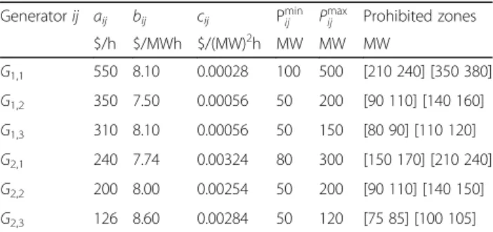
This system consists of two areas. Each area consists of three generators with prohibited operating zones. Transmission loss is considered here. The generator data has modified from [21]. The generator data and B-coefficients are given in the Appendix 1. The percentage of the total load demand in area 1 is 60% and 40% in area 2. The total load demand is 1263 MW and power flow limit of the system is 100 MW.

The problem is solved by using DE, EP, RCGA, and SA. In case of DE, the population size, scaling factor, and crossover rate have been selected as 100, 0.75, and 1.0 re-spectively for the test system under consideration. The population size and scaling factor have been selected as 100, and 0.1 respectively in case of EP. In case of RCGA, the population size, crossover and mutation probabilities have been selected as 100, 0.9 and 0.2 respectively.

Maximum number of generations has been selected 100 for all the four metaheuristic techniques discussed in this paper.

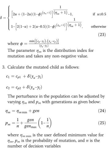
Results obtained from the four metaheuristic techniques i.e. DE, EP, RCGA, and SA have been summarized in Table 1. Figure 1 gives the comparison of convergence of minimum total cost obtained by DE, EP, RCGA, and SA.

4.5.2 Test system 2

This system comprises ten generators with valve-point loading and multi-fuel sources having three fuel options. Transmission loss is considered here. The generator data has been taken from [13]. The total load demand is 2700 MW. The ten generators are divided into three areas. Area 1 consists of the first four units; area 2 includes the next three units and area 3 includes the last three units. The load demand in area 1 is assumed as 50% of the total de-mand. The load demand in area 2 is assumed as 25% and in area 3 is taken as 25% of the total demand. The power flow limit from area 1 to area 2 or from area 2 to area 1 is 100 MW. The power flow limit from area 1 to area 3 or from area 3 to area 1 is 100 MW. Also the power flow limit from area 2 to area 3 or from area 3 to area 2 is 100 MW. The B-coefficients are given in the Appendix 2.

The problem is solved by using four metaheuristic techniques i.e. DE, EP, RCGA, and SA.

In case of DE, the population size, scaling factor, and cross-over rate have been selected as 200, 0.75, and 1.0 respectively for the test system under consideration. The population size and scaling factor have been selected as 100, and 0.1 respect-ively in case of EP. In case of RCGA, the population size, crossover and mutation probabilities have been selected as 100, 0.9 and 0.2 respectively. Maximum number of genera-tions has been selected 300 for DE, EP, RCGA, and SA. 0 50 100 150 200 250 300 350 400 450 500

1.2 1.22 1.24 1.26 1.28 1.3 1.32 1.34x 10

5

)

$(t

s

o

C

Generation

DE

SA EP RCGA

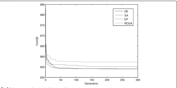
Results obtained from DE, EP, RCGA and RCGA have been presented in Table 2. The cost convergence charac-teristic of this test system obtained from DE, EP, RCGA and SA is shown in Fig. 2.

4.5.3 Test system 3

This system comprises forty generators with valve-point load-ing. The generator data has been taken from [22]. The total load demand is 10500 MW. The forty generators are divided into four areas. Area 1 includes first ten units and 15% of the total load demand. Area 2 has second ten generators and 40% of the total load demand. Area 3 consists of third ten generators and 30% of the total load demand. Area four in-cludes last ten generators and 15% of the total load demand. The power flow limit from area 1 to area 2 or from area 2 to area 1 is 200 MW. The power flow limit from area 1 to area 3 or from area 3 to area 1 is 200 MW. The power flow limit from area 2 to area 3 or from area 3 to area 2 is 200 MW. The power flow limit from area 4 to area 1 or from area 1 to area 4 is 100 MW. The power flow limit from area 4 to area 2 or from area 2 to area 4 is 100 MW. The power flow limit from area 4 to area 3 or from area 3 to area 4 is 100 MW.

Transmission loss is neglected here.

Four metaheuristic techniques i.e. DE, EP, RCGA, and SA have been used to solve the problem.

The population size, scaling factor, and crossover rate have been been selected as 400, 0.75 and 1.0 respectively in case of DE. In EP, the population size and scaling factor have been se-lected 200 and 0.1 respectively. In case of RCGA, the popula-tion size, crossover and mutapopula-tion probabilities have been selected as 200, 0.9 and 0.2 respectively. Maximum number of generations has been selected 500 for DE, EP, RCGA and SA.

Results obtained from DE, EP, RCGA and SA have been depicted in Table 3. The cost convergence characteristic of this test system obtained from DE, EP, RCGA and SA is shown in Fig. 3.

From Tables 1, 2 and 3, it can be inferred that, the low-est minimum total cost amongst the four is achieved by DE, followed by SA. Minimum total cost obtained by EP is more than DE and SA. RCGA is the worst performer. The CPU time requirement is least in case of SA and highest in the case of RCGA amongst the four metaheur-istic techniques discussed in the paper.

5 Conclusion

In this paper, a comparison analysis has been done for the four metaheuristic techniques viz., differential evolution, evolutionary programming, real coded genetic algorithm and simulated annealing technique for multi-area economic dispatch problem considering transmission losses, multiple fuels, valve-point loading and prohibited operating zones with respect to minimum cost and CPU time. Differential evolution achieves the lowest minimum cost and SA requires least CPU time amongst the four metaheuristic techniques.

6 Appendix 1

The transmission loss formula coefficients of two-area system are:

B1¼

17 12 7

12 14 9

7 9 31

2 4

3

5 X10−6

B01¼½−0:3908 −0:1297 0:7047 X10−3

B001 ¼ 0:045

B2¼

24

−6

−8

−6 129

−2

−8

−2 150

2 4

3

5 X10−6

B02¼½0:0591 0:2161 −0:6635 X10−3

B002 ¼ 0:056

7 Appendix 2

The transmission loss formula coefficients of three-area system are:

B1¼

8:70 0:43 −4:61

0:36

0:43 8:30 −0:97

0:22

−4:61 −0:97 9:00 −2:00

0:36 0:22 −2:00

5:30 2

6 6 4

3 7 7

5 X10−5

B01¼ ½−0:3908 −0:1297 0:7047 0:0591 X10−3

B001 ¼ 0:056

B2¼

8:60

−0:80 0:37

−0:80 9:08

−4:90

0:37

−4:90 8:24

2 4

3

5 X10−5

B02¼ ½0:2161 −0:6635 0:5034 X10−3

B002 ¼ 0:045

Table 4Data for 2 area system

Generatorij aij bij cij Pminij Ρ

max

ij Prohibited zones

$/h $/MWh $/(MW)2h MW MW MW

G1,1 550 8.10 0.00028 100 500 [210 240] [350 380]

G1,2 350 7.50 0.00056 50 200 [90 110] [140 160]

G1,3 310 8.10 0.00056 50 150 [80 90] [110 120]

G2,1 240 7.74 0.00324 80 300 [150 170] [210 240]

G2,2 200 8.00 0.00254 50 200 [90 110] [140 150]

B3¼ 1:20

−0:96 0:56

−0:96 4:93

−0:30

0:56

−0:30 5:99

2 4

3

5 X10−5

B03¼ ½−0:3216 0:4635 0:3503 X10−3

B003 ¼ 0:055

Funding

There is NO Funding Information available for this manuscript.

Authors’contributions

JKP makes substantial contributions to conception, design and acquisition of data analysis and interpretation of data. JKP drafted the article and revising it thoroughly for preparation of the manuscript for the esteemed journal. Also he did the simulation part by using different test data for three different test systems. As a corresponding author he takes the primary responsibility for communication of the journal during the manuscript submission, peer review, publication process, and typically ensures that all the journal’s administrative requirements, such as providing details of authorship. JKP will be available throughout the submission and peer review process to respond to editorial queries in a timely manner. Also he will be available after publication to respond to critiques of the work and cooperate with any requests from the journal for data or additional information should be answered about the paper arise after publication. JKP also agrees to be accountable for all aspects of the work in ensuring that questions related to the accuracy or integrity of any part of the work are appropriately investigated and resolved. MB participated in the peer review process of the manuscript and involved in the test data preparation. She reviewed the manuscript thoroughly. DPD participated in the peer review process of the manuscript and to compare the performance of the proposed method with that of other evolutionary methods. All authors read and approved the final manuscript.

Authors_’information

Jagat Kishore Pattanaik received the Master’s degree in Electrical Engineering in 2011 from Jadavpur University, Kolkata, India. He is currently working towards the Ph.D degree in the Department of Power Engineering, Jadavpur University. His research interest is Soft computing application in Power system Engineering.

Dr. Mousumi Basu received the Ph.D. degree from Jadavpur University, Kolkata, India. She is currently working as an Associate Professor in the Department of Power Engineering, Jadavpur University. His research interest is Power system Optimization and Soft computing technique.

Dr. Deba Prasad Dash received the Ph.D. degree from Jadavpur University, Kolkata, India. He is currently working as a Professor in the Department of Electrical Engineering, Orissa Engineering College, Bhubaneswar, Odisha, India. His research interests are Power system Stability, Power system protection & Soft computing technique.

Competing interests

We have declared that we have NO significant competing financial, professional or personal interests that might have influenced the performance or presentation of the work described in the manuscript.

Author details 1

Department of Power Engineering, Jadavpur University, Salt Lake City, Kolkata 700098, India.2_{Electrical Engineering Department, Orissa Engineering}

College, Bhubaneswar, India.

Received: 3 July 2016 Accepted: 18 April 2017

References

1. Shoults, R. R., Chang, S. K., Helmick, S., & Grady, W. M. (1980). A practical approach to unit commitment, economic dispatch and savings allocation for multiple-area pool operation with import/export constraints.IEEE Trans Power Apparatus Syst., 99(2), 625–635.

2. Romano, R., Quintana, V. H., Lopez, R., & Valadez, V. (1981). Constrained economic dispatch of multi-area systems using the Dantzig_–Wolfe decomposition principle.IEEE Trans. Power Apparatus Syst., 100(4), 2127–2137. 3. Desell, A. L., McClelland, E. C., Tammar, K., & Van Horne, P. R. (1984).

Transmission constrained production cost analysis in power system planning.IEEE Trans Power Apparatus Syst., 103(8), 2192_–2198. 4. Helmick, S. D., & Shoults, R. R. (1985). A practical approach to an interim

multi-area economic dispatch using limited computer resources.IEEE Trans Power Apparatus Syst., 104(6), 1400–1404.

5. Wang, C., & Shahidehpour, S. M. (1992). A decomposition approach to non-linear multi area generation scheduling with tie-line constraints using expert systems.IEEE Transactions on Power Systems, 7(4), 1409–1418. 6. Streiffert, D. (1995). Multi-area economic dispatch with tie line constraints.

IEEE Transactions on Power Systems, 10(4), 1946_–1951.

7. Wernerus, J, Soder, L (1995) Area price based multi-area economic dispatch with tie line losses and constraints. In: IEEE/KTH Stockholm power tech conference (pp. 710–715). Sweden

8. Yalcinoz, T., & Short, M. J. (1998). Neural networks approach for solving economic dispatch problem with transmission capacity constraints.IEEE Transactions on Power Systems, 13(2), 307–313.

9. Jayabarathi, T., Sadasivam, G., & Ramachandran, V. (2000). Evolutionary programming based multi-area economic dispatch with tie line constraints. Electric Machine and Power System, 28, 1165–1176.

10. Chen, C. L., & Chen, N. (2001). Direct Search Method for solving Economic Dispatch Problem Considering Transmission Capacity Constraints.IEEE Transactions on Power Systems, 16(4), 764_–769.

11. Chen, C. L. (2005). Optimal generation and reserve dispatch in a multi-area competitive market using a hybrid direct search method.Energy Conversion and Management, 46, 2856–2872.

12. Walter, D. C., & Sheble, G. B. (1993). Genetic algorithm solution of economic dispatch with valve point loading.IEEE Transactions on Power Systems, 8, 1325–1332.

13. Chiang, C.-L. (2005). Improved genetic algorithm for power economic dispatch of units with valve-point effects and multiple fuels.IEEE Transactions on Power Systems, 20(4), 1690–1699.

14. Storn, R., & Price, K. V. (1997). Differential evolution- a simple and efficient heuristic for global optimization over continuous spaces.Journal of Global Optimization, 11(4), 341_–359.

15. Price, K. V., Storn, R., & Lampinen, J. (2005).Differential Evolution: A Practical Approach to Global Optimization. Berlin: Springer.

16. Yang, H. T., Yang, P. C., & Huang, C. L. (1996). Evolutionary Programming based economic dispatch for units with non-smooth fuel cost functions. IEEE transactions on Power Systems, 11(1), 112–118.

17. Goldberg, D. (1989).Genetic Algorithms in Search, Optimization & Machine Learning. Reading: Addison-Wesley Publishing Company, Inc.

18. Deb, K., & Agrawal, R. B. (1995). Simulated binary crossover for continuous search space.Complex Systems, 9(2), 115–148.

19. Kirkpatrick, S., Gelatt, C., & Vecchi, M. (1983). Optimization by simulated annealing.Science, 22, 671–680.

20. Wong, K. P., & Fung, C. C. (1993). Simulated annealing based economic dispatch algorithm.IEE Proceedings Generation Transmission and Distribution, 140(6), 509–515.

21. Gaing, Z.-L. (2003). Particle Swarm Optimization to Solving the Economic Dispatch Considering the Generator Constraints.IEEE Transactions on Power Systems, 18(3), 1187–1195.