Biometrics. 2019;1–11. wileyonlinelibrary.com/journal/biom © 2019 The International Biometric Society 1
count data in the presence of informative dropout
Guoqing Diao
1|
Donglin Zeng
2|
Kuolung Hu
3|
Joseph G. Ibrahim
21Department of Statistics, George Mason
University, Fairfax, VA
2Department of Biostatistics, University of
North Carolina at Chapel Hill, Chapel Hill, NC
3Amgen Inc, Thousand Oaks, CA
Correspondence
Guoqing Diao, Department of Statistics, George Mason University, Fairfax, VA 22030.
Email: [email protected]
Abstract
Recurrent events data are commonly encountered in medical studies. In many applications, only the number of events during the follow‐up period rather than the recurrent event times is available. Two important challenges arise in such studies: (a) a substantial portion of subjects may not experience the event, and (b) we may not observe the event count for the entire study period due to informative dropout. To address the first challenge, we assume that underlying population consists of two subpopulations: a subpopulation nonsusceptible to the event of interest and a subpopulation susceptible to the event of interest. In the susceptible subpopulation, the event count is assumed to follow a Poisson distribution given the follow‐up time and the subject‐specific characteristics. We then introduce a frailty to account for informative dropout. The proposed semiparametric frailty models consist of three submodels: (a) a logistic regression model for the probability such that a subject belongs to the nonsusceptible subpopulation; (b) a nonhomogeneous Poisson process model with an unspecified baseline rate function; and (c) a Cox model for the informative dropout time. We develop likelihood‐based estimation and inference procedures. The maximum likelihood estimators are shown to be consistent. Additionally, the proposed estimators of the finite‐dimensional parameters are asymptotically normal and the covariance matrix attains the semiparametric efficiency bound. Simulation studies demonstrate that the proposed methodologies perform well in practical situations. We apply the proposed methods to a clinical trial on patients with myelodysplastic syndromes.
K E Y W O R D S
Cox model, informative dropout, nonparametric maximum likelihood estimators, nonhomogeneous Poisson process, semiparametric efficiency, zero‐inflated Poisson model
1
|
INTRODUCTION
Recurrent event data are frequently encountered in medical studies. Examples of recurrent events include relapses of multiple sclerosis, admissions to hospitals, occurrences of red blood transfusions, falls in elderly
Our work is motivated by a phase 2, multicenter, randomized, double‐blinded clinical trial with low risk or intermediate myelodysplastic syndromes (MDS) patients who have severe thrombocytopenia (platelet count <50 × 109/L). MDS are malignant diseases of bone‐ marrow stem cells due to ineffective hematopoiesis and dysplastic bone‐marrow morphology (Sloand, 2008). The disease leads to peripheral‐blood cytopenias and in many
patients, progression to acute myeloid leukemia. Platelet transfusion interventions are commonly utilized in terms of bleeding event occurring among these patients. The main objective of the trial is to evaluate whether the investigational product reduces the rate of platelet transfusions and bleeding adverse events reported during the 26‐week study period.
Several important issues arise from the motivating example. First, as is shown in Figure 1, an excess portion of patients have a zero event count (26% and 49% in the placebo group and the treatment group, respectively). Particularly there is a spike at zero for the treatment group. Second, the scatter plot of exposure time vs event count displayed in Figure 2 suggests that the event rate is likely not proportional to the exposure time. Moreover, patients may discontinue the treatment and dropout of study due to disease progression, death or other types of adverse events, which are associated with the event of interest, leading to informative dropout. Finally, in this trial, only the number of recurrent events during the follow‐up period rather than the recurrent event times is available.
When the recurrent event times are observed, there is a large collection of literature on the analysis of recurrent event data in the presence of informative follow‐up times. Cook and Lawless (1997) and Ghosh and Lin (2000; 2002; 2003) proposed marginal models. Alternatively, several authors proposed to jointly model the recurrent events and informative follow‐up time through shared frailty or F I G U R E 1 Frequencies of event count data in the placebo
group (upper panel) and the treatment group (lower panel) from the myelodysplastic syndrome trial
random effects models; for example, see Wang et al. (2001), Huang and Wang (2004), Liuet al. (2004), Yeet al. (2007), Liu and Huang (2009), Zeng and Lin (2009), Zhao et al. (2012), and Liu et al. (2016). In particular, Wang et al. (2001) and Huang and Wang (2004) proposed a shared frailty model without imposing distributional assumptions on the frailty. Another attractive feature of the methods is that the shared frailty is allowed to take value 0 which corresponds to the nonsusceptible subpopulation. On the other hand, Liu et al. (2016) proposed a joint frailty model for zero‐inflated event count data with informative censoring. The joint model consists of a logistic model for the probability of cure (i.e., the patient will not experience the event of interest), a proportional rates model for recurrent event among those “not cured,” and a proportional hazards model for the terminal event. A shared log‐normal frailty is used to account for the correlation between the recurrent events and the terminal event.
All the aforementioned methods assume that the recurrent event times are available. However, in many applications including the motivating example, we do not observe when the recurrent event occurs and instead only the information on the number of recurrent events during the follow‐up period is available. None of the above methods are applicable in such situations. When only the event count data are available, one can consider the zero‐inflated Poisson model (Lambert, 1992; Long, 1997; Cameron and Trivedi, 2013) or zero‐inflated negative binomial models (Long, 1997; Ridout et al., 2001; Yanget al., 2012) to account for the excess number of zero event counts.
The above zero‐inflated Poisson or negative binomial models assume a parametric form of the count data and that the follow‐up time is not informative. That is, the follow‐up time is independent of the event process given the baseline covariates. However, this assumption is violated in several applications including the motivating MDS trial; for instance, see Zhang and Jamshidian (2003), Huang et al. (2006), Sun et al. (2007), He et al. (2009), Zhao and Tong (2011), Zhao et al. (2013), and Diao et al. (2017). None of these methods accounts for excess zeros.
In this paper, we propose a joint semiparametric frailty model to overcome the limitations of existing methods and address the important issues arising in many clinical trials: (a) excess zeros; (b) nonproportionality of the event rate; (c) informative dropout; and (d) unobserved recurrent event times. Specifically, the joint model consists of three components: (a) a logistic regression model for the probability such that a subject will never experience the event of interest; (b) a nonhomogeneous Poisson process for the event data in which the baseline event rate
function is unspecified; and (c) a Cox proportional hazard model for the dropout time. To account for the informative dropout, a shared frailty is introduced in the nonhomo-geneous Poisson model and the Cox model. We develop likelihood‐based estimation and inference procedures. The joint model is similar to the one in Liu et al. (2016); however, it is not trivial to extend the method of Liuet al. (2016) when the recurrent event times are not available. First of all, although the nonparametric maximum like-lihood estimator (NPMLE) of the baseline event rate function is a step function under both scenarios, the jumps can only happen at the observed follow‐up times and there may be no jumps at some observed follow‐up times when the recurrent event times are not available. Second, the proof of the asymptotic properties of the estimators is very much involved and one cannot achieve the usual root‐n convergence rate for the estimator of the unknown baseline event rate function.
The rest of this paper is organized as follows. In Section 2, we introduce the joint semiparametric frailty models. We derive the nonparametric likelihood function of the unknown parameters. Additionally, we describe two algorithms for calculating the NPMLEs. In Section 3, we establish the asymptotic properties of the proposed NPMLEs. Simulation results are provided in Section 4. We apply the proposed methodology to the motivating MDS clinical trial in Section 5. We conclude the paper with some discussions in Section 6.
2
|
METHODS
2.1
|
Semiparametric frailty models
Suppose that there are n subjects. For the ith subject, i= 1, …,n, let Zi denote ad × 1 vector of covariates at baseline;Ciis the administrating censoring time;T∼i is thepotentially informative dropout time; and N t()i is the
event count by time pointt. Therefore, the observed data consist ofOi≡ { , = min ( , ), Δ = (Zi Ti T C∼i i i I T∼i ≤C Xi), =i
N Ti( ) }i ,i= 1,…n, where theTi’s are the observed follow‐
up times and Δi’s are the corresponding censoring indicators. Denote by τ the end of study.
To model excess zero counts, we assume that the underlying population consists of a nonsusceptible subpopulation and a susceptible subpopulation over the [0,τ] interval. We postulate a logistic regression model for the probability such that a subject belongs to the nonsusceptible subpopulation:
∣
∼ ∼
( )
( )
γ γ Y P U( = 1 Z) = exp Z
1 + exp ,
i i
T i
where Ui is a latent variable indicating whether theith
subject belongs to the nonsusceptible subpopulation, ∼
Zi= (1, )Zi , and γ is a vector of regression coefficients
including the intercept.
Second, we assume that subjects in the susceptible subpopulation are from a (conditional) Poisson distribu-tion given that U = 0i and a frailty. Specifically, we
assume that
∣
}
}
{
{
P N t k ξ U
k ξ G t ξ G t
Z
( ( ) = , , = 0)
= 1! ( ) eβ exp − ( ) eβ ,
i i i i
i T iZ k i T iZ (2)
where ξi is a subject‐specific random effect (frailty) representing the subject’s heterogeneity due to other characteristics,G ( )⋅ is an unknown increasing function in [0, ]τ with G (0) = 0, and β is a set of regression coefficients. Model (2) implies that subjects in the susceptible subpopulation follow a conditional Poisson distribution with meanξ G T( ) eβ
i i T iZ. Consequently,N t()i
is a (conditional) nonhomogeneous Poisson process with rate functionξ G t() eβ
i T iZ.
Finally, we assume that T∼i is independent of N t()i givenξi and
∣
∼ ζ
P T( >i t ξi, ) = exp {−Zi ξ H ti ( ) exp ( TZi) }, (3)
where H t() is a strictly monotone increasing but otherwise unspecified function, and ζ is a set of regression coefficients. Model (3) is referred to as the Cox model with a shared frailty (Murphy, 1994; 1995).
For ease of presentation, we have used the same set of covariates Zi in models (1) to (3). However, it is straightforward to extend them to allow for different sets of covariates, which may or may not contain common components. The shared frailtyξiin models (2) and (3) is used to account for informative dropout. The positive correlation between the event rate and the hazard rate of the dropout time suggests that patients who experience more events tend to be at a higher risk of dropout and vice versa. This is a reasonable assumption which was validated by several real applications (Zeng et al., 2014; Yuet al., 2016). A common choice for the distribution of the frailty is the γ distribution, although other distribu-tions such as the log‐normal distribution and the positive stable distribution can also be considered. For the ease of computation, we assume thatξi’s are i.i.dγwith mean 1 and variance θ. The mean of the γ frailty ξi is fixed to ensure model identifiability.
The unknown parameters include γ β, , , , ( )θ ζ G t , and H t(), t ∈[0, ]τ. It is worth to note that there are two infinite‐dimensional parameters in the joint models,
⋅
G ( ) and H ( )⋅ , which present challenges in both the numerical implementation and the theoretical develop-ment of the estimators. Writeϕ= ( , , , )γ β θ ζ . We assume that the censoring timeCiis conditionally independent ofT∼i
given Zi. Based on the observed data, the likelihood
function for the unknown parameters( , , )ϕ G H is
where h ( )⋅ is the first derivative of H ( )⋅ , and
∕
f ξ( ) = (θ−θ−1/Γ ( ) )θ−1 ξθ−1−1 −e ξ θ is the γ θ θ( ,−1 −1)
den-sity. With some algebra, we can show that Ln( , , ) =ϕ G H ∏ni=1 {∑3j=1M3( ; , , ) },Oi ϕ G H where
∫
∏
∼∼ ∼ ∼{
}
( )
( )
( )
( )
{
}
{
} {
}
{
}
{
}
ϕ γ γ γ γL G H I X ξ G T
I X ξ G T ξ G T
X ξ h T ξ H T f ξ dξ
Z
Z Z
Z
( , , ) = ( = 0) exp
1 + exp +
exp − ( ) e 1 + exp
+ ( > 0) ( ) e exp − ( ) e
1 + exp ! × ( ) e exp − ( ) e ( ) ,
β β β ζ ζ n i n ξ i T i T i i i T i i i
i X i i
T i i i i
Δ
i i i i
Z
Z Z
Z Z
=1 i
T i
T i i T i
T i i T i
⎛ ⎝ ⎜ ⎜ ⎜ ⎡ ⎣ ⎢ ⎢ ⎢ ⎤ ⎦ ⎥ ⎥ ⎥ ⎧ ⎨ ⎪ ⎩⎪ ⎫ ⎬ ⎪ ⎭⎪ ⎞ ⎠ ⎟ ⎟ ⎟ ∼ ∼ ∼
{
}
{
}
( )
( )
(
)
( )
{
}
{
}
{
}
{
}
φ γ γ φ γM G H I X h T
θ H T
M G H I X h T
θ G T H T
O Z
Z
O
Z
( ; , , ) = ( = 0) exp ( ) e
1 + exp 1 + ( ) e
( ; , , ) = = 0 ( ) e
1 + exp 1 + ( ) e + ( ) e
ζ
ζ
ζ
β ζ
i i
T i i
T i i θ
i i i
T i i i θ
Z Z Z Z Z 1 Δ +Δ 1 Δ +Δ
T i i
T i i
T i i
T i T i i
and
Naturally one would like to maximize the above likelihood Ln( , , )ϕ G H to estimate the unknown para-meters. However, the maximum likelihood does not exist since for any fixed H t(), one can always let h t() go to infinity at an observed time point ofT∼. Therefore, we use the nonparametric maximum likelihood approach as in Murphy (1994) allowing both G and H to be right continuous and replacingh t()with the jump size ofH ( )⋅ at t. For ease of notation, we also denote the resulting nonparametric likelihood by Ln( , , )ϕ G H . It can be shown that the NPMLE of H is a step function with jumps only at the observed time points ofT∼. The NPMLE ofG ( )⋅ , however, is not unique since the nonparametric likelihood depends on G only through its values at the observed exposure times T ii, = 1, …,n, so we focus on the maximization of Ln( , , )ϕ G H over all nondecreasing step functions with jumps at theTi’s forG t().
Although there is a closed form for the observed‐data nonparametric likelihood function, it is still challenging to maximize Ln( , , )ϕ G H as it involves two infinite‐ dimensional parameters in G and H and a set of finite‐ dimensional parametersϕ. To address this computational issue, we describe an EM algorithm in the next section.
2.2
|
An EM algorithm
We now describe an EM algorithm for maximizing the observed‐data likelihood. Recall that we define a binary latent variable Ui such that U = 1i if Xi belongs to a
subpopulation with a point mass at 0 andU = 0i if Xi
belongs to a subpopulation that follows a conditional Poisson distribution. The complete‐data likelihood based on{ ( , , ), = 1, …, }Oi U ξ ii i n is
It can be shown that, given the observed data Oi and current parameter estimates ( , , )ϕ G H , Ui follows a
Bernoulli distribution with success probability ∑
ϕ ϕ
pi =M1( ; , , )/Oi G H 2j=1Mj( ; , , )Oi G H if X = 0i
and U = 0i with probability one if X > 0i . Further-more, it can be shown that givenUi= 0,Oi, and the
cur-rent parameter estimates, ξ ∼Γ
(
θ + Δ , ( ) eG T βi −1 i i TZi
)
H T θ
+ ( ) e i ζTZi+ −1 if Xi= 0 and ξ ∼Γ
(
θ +Xi −1 i
)
G T H T θ
+Δ , ( ) ei i βTZi+ ( ) ei ζTZi + −1 ifX > 0i . Similarly, given U = 1i , Oi, and the current parameter estimates,
∼
(
)
ξ Γ θ + Δ , ( ) eH T ζ +θ
i −1 i i Z −1
T i
.
Therefore, given the observed data and current parameter estimates ( , , )ϕ G H , we can maximize the
conditional log‐likelihood ∑in=1 E{logLn iC, ( , , )ϕ G H ∣O , , , },i ϕ G H where Ln iC, ( , , )ϕ G H is the complete‐data likelihood contributed from theith subject.
Based on the conditional distribution of( , )ξ Ui i given
the observed dataOiand current parameter estimates, we can derive a closed form for the above conditional log‐ likelihood. In particular, it can be written as the sum of four separate terms: likelihood from a standard logistic regression, likelihood from a Cox model for the informative dropout time, likelihood from a nonhomo-geneous Poisson process for panel count data, and a term involving the variance parameterθ. These four terms can be maximized separately in the M‐step of the EM algorithm. It is a standard practice to update the estimates of γ ζ, , and H ( )⋅ in the M‐step. To update the estimates ofβandG ( )⋅ , one can use an optimization algorithm or the pool adjacent violator algorithm (PAVA) (Barlow et al., 1972; Robertsonet al., 1988).
2.3
|
An alternative algorithm
One drawback of the above EM algorithm is that optimization algorithms or the PAVA are needed to
∏
∼∼ ∼ ∼( )
( )
(
)
( )
{
} {
( )
}
{
}
{
}
{
}
{
}
ϕ γ γ γ γL G H U I X ξ h T ξ H T f ξ
U I X ξ G T I X ξ G T ξ G T
X
ξ h T ξ H T f ξ
Z Z
Z Z
( , , ) = ( = 0) exp
1 + exp ( ) e exp − ( ) e ( )
+ (1 − ) ( = 0)exp − ( ) e
1 + exp + ( > 0)
( ) e exp − ( ) e
{1 + exp } !
× ( ) e exp − ( ) e ( )
ζ ζ
β β β
ζ ζ nC i n i i T i
T i i i i i i
i i i iT
i
i i i
X
i i T i i
i i i A i i
Z Z
Z Z Z
Z Z
=1
Δ
Δ
T i i T i
T i T i i T i
T i i
i T i
⎡ ⎣ ⎢ ⎢ ⎢ ⎤ ⎦ ⎥ ⎥ ⎥ ∼
{
( )
}
{
}
{
}
ϕ γM G H I X G TX h T θ θX
θ
θ G T H T
O
Z
( ; , , ) = ( > 0) ( )! e ( ) e Γ ( Γ ( )+ + Δ )
×
1 + exp 1 + ( ) e + ( ) e .
β ζ
β ζ
i i i
X i
X i i i
X
T i i i θ X
Z Z Z Z 3 Δ −1 −1 +Δ + +Δ i
i T i T i i
i i
T i T i −1 i i
⎡
estimate G ( )⋅ in the M‐step. Therefore, two loops of iterations are involved in the EM algorithm leading to an expensive computational burden. Alternatively, we con-sider an optimization algorithm to maximize the observed‐data likelihood directly. The main challenge is that both the estimates ofG ( )⋅ andH ( )⋅ are constrained to be nondecreasing. To alleviate the constrained optimization problem, we use the following transforma-tion (of the parameters): H t( ) =k ∑kj=1exp ( ), = 1,α kj
m
…, H, and G s( ) =k ∑kj=1exp ( ), = 1, …,δ kj mG, where
⋯
t1< <t2 <tmH are the distinct observed dropout times and s1< <s2 ⋯<smG are the distinct observed exposure times. The new parameters αj and δj are
the jumps of H ( )⋅ and G ( )⋅ at tj and sj, respectively.
A similar transformation technique was also used by Zeng et al. (2006) for the analysis of intercensored data and more recently by Diao and Yuan (2019) for the analysis of current status data with a cured fraction. We then maximize the observed‐data likelihood over
ϕ α α δ δ
( , , …,1 mH, , …,1 mG) without constraints by using the Broyden‐Fletcher‐Goldfarb‐Shanno algorithm (BFGS) algorithm as described in Presset al. (1992). Throughout the numerical studies, the results are obtained based on this direct optimization algorithm.
3
|
ASYMPTOTIC PROPERTIES
In this section, we establish the asymptotic properties of the proposed NPMLEs of the unknown parameters( , , )ϕ G H , denoted by( , , )ϕ G H n n n . Supporting Information Appendix
A lists the necessary assumptions. In Supporting Informa-tion Appendix B, we prove that if two sets of parameters
∈
ϕ G t H t t τ
( , ( ), ( ), [0, ] ) and ( , ( ), ( ),ϕ G t H t t͠ ∼ ∼ ∈[0, ] )τ give the same likelihood for the observed data O, then
͠
ϕ ϕ= ,G t( ) = ( )G t∼ , and H t( ) = ( )∼H t for anyt∈ [0, ]τ . Therefore, the proposed model is identifiable.
Define
∣ ∣ ∣ ∣
∣ ∣
∣ ∣
∈
ϕ ϕ ϕ ϕ
d G H G H
G t G t
H t H t
{ ( , , ), ( , , ) } = −
+ sup { ( ) − ( )
+ ( ) − ( ) }
t τ
0 0 0 0
[0, ] 0
0
where∣ ∣ ⋅∣ ∣is the Euclidean norm. Here( , , )ϕ G H0 0 0 are the true parameters values as defined in Supporting Information Appendix A. We now prove that( , , )ϕ G H n n n
is consistent.
Theorem 1. Under the conditional independent censoring assumption and assumptions (C1) to (C4) in Supporting Information Appendix A, d{ ( , , ),ϕ n G Hn n
→
ϕ G H
( , , ) }0 0 0 0 almost surely.
The proof of Theorem 1 involves the proof of the P‐ Glivenko‐Cantelli property for some classes. Specifically,
we will prove the class k≡{ (m O∣ϕ, , ): ( , , )G H ϕ G H ∈` f f× × } is a P‐Glivenko‐Cantelli class, where
∣ϕ ∣ϕ ∣ϕ
m(O , , ) = log (G H p O , , ) − log (G H p O 0, , )G H0 0 is
the log‐likelihood ratio and p(O∣ϕ, , )G H is the likelihood based on a single observationO as defined in Supporting Information Appendix B. By Theorem 5.8 in van der Vaart (2002), we can then show that
→
ϕ ϕ
d{ ( , , ), ( , , ) } n G Hn n 0 G H0 0 0 almost surely. Detailed proof is provided in Supporting Information Appendix C. With the consistency result, we next derive the convergence rate of ( , , )ϕ G H n n n and the asymptotic
normality property forϕn.
Theorem 2. Under the conditional independent censoring assumption and assumptions (C1) to (C4) in Supporting Information Appendix A, d{ ( , , ),ϕ n G Hn n
∕
ϕ G H O n
( , , ) } =0 0 0 p( −1 3).
Theorem 3. Under the conditional independent censoring assumption and assumptions (C1) to (C4) in Supporting Information Appendix A, n ( − )ϕn ϕ0 converges weakly to a (3 + 2) × 1d normal random vector with mean zero and a covariance matrix attaining the semiparametric efficiency bound.
Remark1. Theorem 2 implies that the NPMLEs have a slower convergence rate than root‐n. To derive this result, we verify the conditions of Theorem 3.4.1 in van der Vaart and Wellner (1996). Theorem 3 further implies that although( , , )ϕ G H n n n has a cubic root‐nconvergence rate,
ϕn still attains the root‐n convergence rate and is
asymptotically normal. Detailed proof of Theorems 2 and 3 is provided in Supporting Information Appendices D and E, respectively.
Remark2. In principle, one can estimate the covariance matrix ofϕnby a plug‐in method replacing the unknown parameters with their NPMLEs in the corresponding analytic form. However, the implementation is very complicated. Therefore, we use the multiplier bootstrap method (Kosorok, 2008, chapter 2) to estimate the covariance matrix of ϕn. The covariance matrix of ϕn is thus estimated by the empirical sample covariance matrix of the bootstrap estimates. Alternatively, one can use the standard bootstrap method (van der Vaart and Wellner, 1996, chapter 3.6). In our experience, the multiplier bootstrap method is numerically more stable particularly for small sample sizes.
provethat underthe conditionalindependentcensoring assumptionandassumptions (C1)to(C4)inSupporting InformationAppendixA,theasymptoticnulldistribution of the likelihood ratio test statistic for testing the null hypothesisofnoninformativedropoutisa50:50 mixture of apointmassat0and χ12.
4
|
SIMULATION
STUDIES
We conduct simulation studies to examine the finite‐ sample performance of the proposed NPMLEs. We generate two covariates: Z1∼Bernoulli(1∕2) and Z2∼ N(0,0.25).Wethengeneratedatabasedonmodels (1) to (3). The true parameters are set to be γ =(−1,−1,0.5),β=(0.5,−0.5), ζ=(−0.5, 0.5), θ=1, G(t) = 2t, and H t()=(t∕5)3∕2. The censoring timefor thedropouttimeissettobeC=6forallsubjects.Under
this simulation setting, approximately 65% of the subjects have zero event counts. For each simulation, we consider sample sizes of 150, 300, and 600. To estimate the covariance matrix of ϕn, we use the multiplier bootstrap method with 400 bootstrap samples. To construct confidence intervals, we first estimate the standard errors based on the bootstrap samples and then apply the asymptotic normality results in Theorem 3. Specifically, the 1 −α confidence interval estimate for ϕ is
∕
ϕn±z SEα 2( )ϕn , where zα 2∕ is the 1 −α∕2 quantile of
N (0, 1).
It is worth noting although the proposed model is identifiable, a data set with a small fraction of zero counts can cause numerical instability and the algorithm may fail to converge. This phenomenon, however, is not unique. In our experience, even for the simple zero‐inflated Poisson regression model, if the proportion of subjects with zero event counts is small, algorithms implemented in standard
T A B L E 1 Summary statistics for the nonparametric maximum likelihood estimators based on 1000 replicates
n Parameters True Est EmpSD Mean SE CP
150 θ−1 1.0 1.426 0.759 0.831 0.978
β1 0.5 0.535 0.344 0.287 0.919
β2 –0.5 –0.506 0.342 0.297 0.921
γ0 0.5 0.450 0.239 0.227 0.952
γ1 –0.5 –0.457 0.404 0.428 0.958
γ2 0.5 0.485 0.422 0.455 0.977
ζ1 –0.5 –0.478 0.299 0.303 0.956
ζ2 0.5 0.500 0.300 0.305 0.955
300 θ−1 1.0 1.229 0.379 0.463 0.976
β1 0.5 0.529 0.217 0.197 0.929
β2 –0.5 –0.520 0.218 0.199 0.923
γ0 0.5 0.481 0.142 0.150 0.964
γ1 –0.5 –0.509 0.270 0.280 0.961
γ2 0.5 0.492 0.285 0.289 0.953
ζ1 –0.5 –0.480 0.202 0.210 0.962
ζ2 0.5 0.496 0.194 0.212 0.967
600 θ−1 1.0 1.127 0.250 0.312 0.975
β1 0.5 0.515 0.146 0.143 0.946
β2 –0.5 –0.518 0.156 0.142 0.921
γ0 0.5 0.484 0.103 0.105 0.954
γ1 –0.5 –0.488 0.193 0.193 0.948
γ2 0.5 0.490 0.194 0.198 0.954
ζ1 –0.5 –0.492 0.141 0.150 0.967
ζ2 0.5 0.491 0.143 0.151 0.963
software packages such as R and SAS can also fail to converge. Indeed, as one referee pointed out, the zero‐ inflated Poisson regression makes little sense if the observed percentage of zero counts is low. Under the above simulation setting, we did not encounter conver-gence problems in the numerical studies.
Table 1 presents the summary statistics of the NPMLEs of the finite‐dimensional parameters based on 1000 replicates. For moderately large sample sizes of 300 and 600, the proposed NPMLEs have low biases, the estimated standard errors obtained from the bootstrap method reflect the actual variation of the estimators, and the coverage probabilities of the 95% confidence intervals obtained based on the bootstrap method and the asymptotic normality results in Theorem 3 are close to the nominal level. As sample size increases from 300 to 600, both biases and coverage probabilities of the 95% confidence interval improve. The standard errors decrease by a factor of 2 suggesting root‐nconvergence rate ofϕn. Under the setting with a smaller sample size of 150, the NPMLEs for all parameters with the exception of the variance of the frailty still perform well. Figure 1 in Supporting Information Appendix F displays the true and estimated curves of the baseline rate function G t() and the baseline cumulative hazard function H t(). The true curves and estimated curves are very close for sample sizes of 300 and 600 suggesting small biases of the estimators of NPMLEs of G t()andH t().
We conduct additional simulation studies to evaluate how sensitive the proposed method is to the frailty distribution misspecification. Specifically, we consider generating the frailty from a log‐normal distribution and an inverse Gaussian distribution, both with mean 1 and variance 1. Detailed results are presented in Tables 1 and 2 in Supporting Information Appendix F. While the estimation of the frailty variance is sensitive to the frailty distribution misspecification, the NPMLEs of the regres-sion parameters are reasonably robust. Figures 2 and 3 in Supporting Information Appendix F show that the estimators ofG t() and H t() have some biases, particu-larly at later time points.
5
|
APPLICATION TO MDS DATA
We apply the proposed methods to the motivating MDS trial, which was conducted in multiple countries with a 2 to 1 randomization ratio (treatment vs. placebo). The randomization was stratified based on baseline platelet counts (25‐50×109/L and below 25×109/L) and disease risk status (low and intermediate‐1). The final data set contains 150 patients, among which 100 were in the treatment group and 50 were in the placebo group. The exposure time ranges from 16 days to 180 days with a median of 113 days in the placebo group and ranges from 7 days to 180 days with a median of 116 days in the treatment group. Thirty‐six treatment patients (36%) and 14 placebo patients (28%) dropped out early during the efficacy follow‐up phase mainly due to alternative therapies that are different from both the treatment and placebo. Log‐rank test shows that there is little difference in the distribution of the dropout time between two treatment groups (P= .677). The total number of bleeding or platelet transfusion events in the placebo group ranges from 0 to 34 with first quartile, median, and third quartile of 0.25, 2, and 11.75. In the treatment group, the event count ranges from 0 to 45 with first quartile, median, and third quartile of 0, 1, and 3.5. Although one patient in the treatment group experienced the event 45 times, the distribution in the placebo group has a heavier right tail and a wider interquartile range.
For comparison, we also analyzed the data using three existing methods, including the method proposed in Diaoet al. (2017) (DZHI), the parametric zero‐inflated Poisson regression model (ZP), and the parametric zero‐ inflated negative binomial model (ZNB). In the para-metric zero‐inflated models, we use the log‐link function and include the logarithm of the dropout time as an intercept. We consider the treatment indicator as the covariate in the model, which takes value 0 for the placebo group and 1 for the treatment group. Both groups have substantial portions of patients with zero event count. We emphasize again that those methods assuming that the recurrent event times are available cannot be used here.
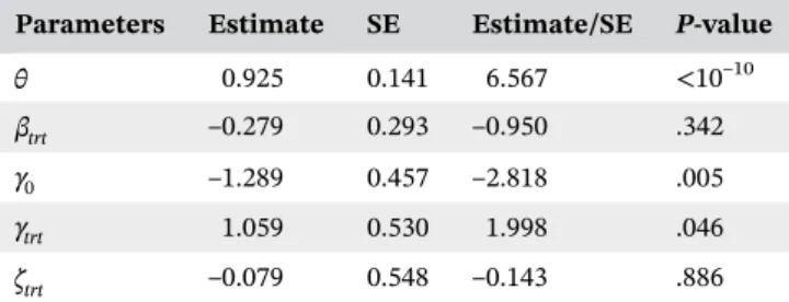
Table 2 presents the results from the MDS trial. The standard errors of the NPMLEs are based on 1000 multiplier bootstrap samples. The variance of theγfrailty is estimated at 0.925 with a standard error of 0.141. These results strongly support the alternative hypothesis of informative dropout and that the event count data and the hazard rate of the dropout time are positively correlated (P< 10−10). There is a significant treatment effect (P= .046) on the probability whether a patient belongs to the nonsusceptible subpopula-tion. The odds for a patient in the treatment group belonging T A B L E 2 Results of the myelodysplastic syndrome trial
Parameters Estimate SE Estimate/SE P‐value
θ 0.925 0.141 6.567 <10–10
βtrt –0.279 0.293 –0.950 .342 γ0 –1.289 0.457 –2.818 .005 γtrt 1.059 0.530 1.998 .046 ζtrt –0.079 0.548 –0.143 .886
ap qi: imixture of a point mass at 0 and a negative binomial distribution with parameters θ + Δ−1 i and success
prob-abilities πi≡G T( ) ei βT iZ/θ−1+G T( ) ei βT iZ + ( ) e ,H Ti ζT iZ
where p = e /(1 + ei γT i∼Z γT i∼Z) and qi = 1 −pi. Therefore, ∣
P X( = 0 , Δ , ) = + (1 − )i Ti i Zi pi qi πi θ +Δ−1 iand fork > 0,
∣
P X k T
q kk θθ π π
Z
( = , Δ , )
= Γ ( +!Γ ( + Δ )+ Δ )(1 − ) .
i i i i i
i
i i
θ ik
−1
−1 +Δi
−1
To check the goodness‐of‐fit of the proposed model, we first categorize the severity of adverse effects to four levels: none (X = 0), mild (1≤ ≤X 5), medium (6≤ ≤X 10), and severe (X > 10). We then compare the goodness‐of‐fit of the proposed method with that of the method of Diao et al. (2017) and the two parametric zero‐inflated models by using the following three statistics for each treatment group: (a) deviance: 2∑k4=1nk log ( / );n μk k (b)
Kullback‐Leibler divergence: 2∑4k=1μk log ( / );μ nk k and (c) Pearson’s χ2 statistic: ∑mk=0 ( ( − ) / ).nk μk 2 μk Here nk
andμkare the observed count and expected count for cell k, respectively. As shown in Table 3, all three goodness‐of‐ fit statistics suggest that the proposed model fits the data better than the three existing methods. Particularly, the proposed method fits the data in the treatment group substantially better than the existing methods since a large portion of patients have zero events.
6
|
DISCUSSION
We have proposed joint semiparametric frailty models for zero‐inflated event count data in the presence of F I G U R E 3 Estimatedbaselinemean
functionG(t)(upperpanel)and estimatedbaselinecumulativehazard functionH t()(lowerpanel)
to the nonsusceptible subpopulation is estimated at 2.89 times (95% confidence interval: 1.02–8.15) the odds for a patient in theplacebo group.Thisresult isconsistentwith the preliminary analysis of the relative frequencies of the patientswithzeroeventcountinthetwogroups.Thereisno significant difference between the two groups for patients whofollowaconditionalPoissondistribution.Thereisalso nosignificantdifference(P=.886)betweenthedistributions of thedropout timeinthetwogroups,whichisconsistent withthelog‐ranktestresult.Figure3displaystheestimates of G t() and H t(). The estimated curve Gn t() does
not appear to be a straight line, suggesting that the event countprocessisnothomogeneous.
Compared to the proposed method, the method of Diao etal.(2017)failed to detectthe difference between thetreatmentgroupandtheplacebogroup.Ontheother hand, the parametric zero‐inflated Poisson model does not account for informative dropout and yields signifi-cant treatment effects on both the probability that a patient belongs to the nonsusceptiblesubpopulationand the event rate for patients inthe Poisson subpopulation with Pvalues .01 and .018, respectively. It is known in statisticalliteraturethatignoringcorrelationsamongdata can lead to an abundance of false positive results. The zero‐inflated negative binomial model appears to yield numerically unstable estimates with the intercept and coefficient for the treatment effect in the logistic model estimated at–10.885and8.972.
Wenextdescribeprocedurestocheckthegoodness‐of‐fitof theproposedmodel.Itcanbeshownthat,conditionalon (T,i Δi, )Zi, Xi follows a zero‐inflated negative binomial
informative dropout. The joint models allow a positive probability such that some patients will never experience the event of interest even after a sufficiently long follow‐ up. Furthermore, the joint models do not require parametric forms of the baseline event rate function of the event count data or the baseline cumulative hazard of the dropout time, and thus gain much flexibility and robustness. Furthermore, a shared frailty is introduced to account for the informative dropout. For the ease of computation complexity, we assume that the frailty follows a γ distribution. Simulation studies demonstrate the NPMLEs of the regression parameters are reasonably robust to the frailty distribution misspecification.
In the logistic regression model (1), we assume that Ui is independent of the frailty ξi, that is,
∣ ∣
P U( = 1 , ) = ( = 1i ξi Zi P Ui Zi). Consequently, the in-dicator Ui whether the ith subject belongs to the
nonsusceptible subpopulation is assumed to be condi-tionally independent of the dropout time T∼i given
covariates Zi. To account for the potential correlation between Ui and T∼i, we may include ξi in the logistic
regression model (1). We may also consider other survival models for the informative dropout time, for example, the proportional odds model (Bennett, 1983), and the short‐term and long‐term hazards/odds rate models (Diaoet al., 2013; Yuan and Diao, 2014). Another limitation of the proposed method is that we assume the recurrent events and the informative dropout share the same frailty. The proposed method may not be applicable if the within‐subject recurrent event correlation and the correlation between the recurrent events and dropout are different. One solution is to use a bivariate frailty to account both types of correlations. The observed‐data likelihood, however, does not have a closed form. Numerical integration or Monte‐Carlo‐based methods will have to be used to maximize the observed‐data likelihood and consequently further increase the already expensive computational burden.
In the real application, we have described several procedures to check the goodness‐of‐fit of the proposed model, which are based on deviance, Kullback‐Leibler divergence and Pearson’s χ2statistic. These procedures, however, are somehow ad hoc and can only be used to compare the fit of different models. It would be desirable to develop formal goodness‐of‐fit procedures to check the model assumptions including the functional forms of the covariates.
We have considered the event count data for one type of event. In many clinical trials, multiple types of adverse events may occur during the treatment period and it is of interest to assess the treatment effects on the multiple event rates. Additional issue arises in such situation. One needs to account for both the correlations among the count data from multiple types of adverse events and the correlations of these event count data with the informa-tive dropout time.
ACKNOWLEDGMENTS
The authors thank the Editor, the Associate Editor, and two anonymous referees for their valuable comments that have improved the presentation of the paper.
ORCID
Guoqing Diao http://orcid.org/0000-0001-7304-9591 Donglin Zeng http://orcid.org/0000-0003-0843-9280
REFERENCES
Barlow, R.E., Bartholomew, D.J., Bremner, J.M. and Brunk, H.D. (1972)Statistical Inference Under Order Restrictions. New York: Wiley.
Bennett, S. (1983) Analysis of survival data by the proportional odds model.Statistics in Medicine, 2, 273–277.
Cameron, A.C. and Trivedi, P.K. (2013). ) Regression Analysis of Count Data. Cambridge, UK: Cambridge University Press. T A B L E 3 Observed and expected frequencies from the myelodysplastic syndrome trial
Placebo Treatment
Count Observations New DZHI (2017) ZP ZNB Observations New DZHI ZP ZNB
0 13 14.097 9.804 12.619 2.4567 49 49.88 23.995 48.7301 21.7206 1‐5 19 14.632 22.194 13.1522 18.7542 28 23.536 51.132 19.4927 45.0795 6‐10 4 9.385 9.671 12.5651 12.7071 10 13.972 16.271 20.0345 21.3796 >10 14 11.886 8.333 11.6637 16.082 13 12.612 8.601 11.7427 11.8203 Deviance 5.583 8.899 10.707 30.686 2.080 37.250 9.570 40.337 KL divergence 6.757 9.788 14.079 25.160 2.183 36.060 10.797 37.835
χ2 4.856 8.680 8.918 51.488 2.003 41.191 8.875 46.906
Cook, R.J. andLawless, J.F. (1997)Marginal analysisof recurrent eventsandaterminatingevent.StatisticsinMedicine,16,911–924. Diao,G.andYuan,A.(2019)Aclassofsemiparametriccuremodels
withcurrentstatusdata.LifetimeDataAnalysis,25,26–51. Diao,G.,Zeng,D.,Hu,K.andIbrahim,J.G.(2017)Modelingevent
count data in the presence of informative dropout with application to bleeding and transfusion events in myelodysplas-tic syndrome.Statistics in Medicine, 36, 3475–3494.
Diao, G., Zeng, D. and Yang, S. (2013) Efficient semiparametric estimation of short‐term and long‐term hazard ratios with right‐ censored data.Biometrics, 69, 840–849.
Ghosh, D. and Lin, D. (2000) Nonparametric analysis of recurrent events and death.Biometrics, 56, 554–562.
Ghosh, D. and Lin, D. (2002) Marginal regression models for recurrent and terminal events.Statistica Sinica, 663–688. Ghosh, D. and Lin, D. (2003) Semiparametric analysis of recurrent
events data in the presence of dependent censoring.Biometrics, 59, 877–885.
He, X., Tong, X. and Sun, J. (2009) Semiparametric analysis of panel count data with correlated observation and follow‐up times.
Lifetime Data Analysis, 15, 177–196.
Huang, C.‐Y. and Wang, M.‐C. (2004) Joint modeling and estimation for recurrent event processes and failure time data.
Journal of the American Statistical Association, 99, 1153–1165. Huang, C.‐Y., Wang, M.‐C. and Zhang, Y. (2006) Analysing panel count
data with informative observation times.Biometrika, 93, 763–775. Kosorok, M.R. (2008) Introduction to Empirical Processes and
Semiparametric Inference. New York: Springer.
Lambert, D. (1992) Zero‐inflated Poisson regression, with an application to defects in manufacturing.Technometrics, 34, 1–14. Liu, L. and Huang, X. (2009) Joint analysis of correlated repeated measures and recurrent events processes in the presence of death, with application to a study on acquired immune deficiency syndrome.Journal of the Royal Statistical Society, 58, 65–81. Liu, L., Huang, X., Yaroshinsky, A. and Cormier, J.N. (2016) Joint
frailty models for zero‐inflated recurrent events in the presence of a terminal event.Biometrics, 72, 204–214.
Liu, L., Wolfe, R.A. and Huang, X. (2004) Shared frailty models for recurrent events and a terminal event.Biometrics, 60, 747–756. Long, S.J. (1997) Regression Models for Categorical and Limited
Dependent Variables. Beverly Hills, CA: Sage Publications. Murphy, S.A. (1994) Consistency in a proportional hazards model
incorporating a random effect.The Annals of Statistics, 22, 712–731. Murphy, S.A. (1995) Asymptotic theory for the frailty model. The
Annals of Statistics, 23, 182–198.
Murphy, S.A. and vanderVaart, A.W. (1997) Semiparametric like-lihood ratio inference.The Annals of Statistics, 25, 1471–1509. Press, W.H., Teukolsky, S.A., Vetterling, W.T. and Flannery, B.P.
(1992)Numerical Recipes in C: The Art of Scientific Computing, Second ed. Cambridge: Cambridge University Press.
Ridout, M., Hinde, J. and DeméAtrio, C.G. (2001) A score test for testing a zero‐inflated poisson regression model against zero‐ inflated negative binomial alternatives.Biometrics, 57, 219–223. Robertson, T., Wright, F. and Dykstra, R. (1988)Order Restricted
Statistical Inference. New York: Wiley.
Sloand, E.M. (2008) Myelodysplastic syndromes: introduction,
Seminars in Hematology. Elsevier Inc., pp. 1–2.
Sun, J., Tong, X. and He, X. (2007) Regression analysis of panel count data with dependent observation times.Biometrics, 63, 1053–1059.
van der Vaart, A. and Wellner, J. (1996)Weak Convergence and Empirical Processes. New York: Springer‐Verlag.
van der Vaart, A.W. (2002) Semiparametric statistics. In:Lectures on Probability Theory and Statistics, Lecture Notes in Math, P. Bernard (ed), New York: Springer, Vol. 1781, pp. 331–457. Wang, M.‐C., Qin, J. and Chiang, C.‐T. (2001) Analyzing recurrent
event data with informative censoring.Journal of the American Statistical Association, 96, 1057–1065.
Yang, J., Li, X. and Liu, G.F. (2012) Analysis of zero‐inflated count data from clinical trials with potential dropouts. Statistics in Biopharmaceutical Research, 4, 273–283.
Ye, Y., Kalbfleisch, J.D. and Schaubel, D.E. (2007) Semiparametric analysis of correlated recurrent and terminal events.Biometrics, 63, 78–87.
Yu, H., Cheng, Y.‐J. and Wang, C.‐Y. (2016) Semiparametric regression estimation for recurrent event data with errors in covariates under informative censoring. The International Journal of Biostatistics, 12.
Yuan, M. and Diao, G. (2014) Semiparametric odds rate model for modeling short‐term and long‐term effects with application to a breast cancer genetic study. The International Journal of Biostatistics, 10, 231–249.
Zeng, D., Cai, J. and Shen, Y. (2006) Semiparametric additive risks model for interval‐censored data.Statistica Sinica, 16, 287–302. Zeng, D., Ibrahim, J.G., Chen, M.‐H., Hu, K. and Jia, C. (2014) Multivariate recurrent events in the presence of multivariate informative censoring with applications to bleeding and transfusion events in myelodysplastic syndrome. Journal of Biopharmaceutical Statistics, 24, 429–442.
Zeng, D. and Lin, D. (2009) Semiparametric transformation models with random effects for joint analysis of recurrent and terminal events.Biometrics, 65, 746–752.
Zhang, Y. and Jamshidian, M. (2003) The Gamma‐frailty Poisson model for the nonparametric estimation of panel count data.
Biometrics, 59, 1099–1106.
Zhao, X., Liu, L., Liu, Y. and Xu, W. (2012) Analysis of multivariate recurrent event data with time‐dependent covariates and informative censoring.Biometrical Journal, 54, 585–599. Zhao, X. and Tong, X. (2011) Semiparametric regression analysis of
panel count data with informative observation times. Computa-tional Statistics and Data Analysis, 55, 291–300.
Zhao, X., Tong, X. and Sun, J. (2013) Robust estimation for panel count data with informative observation times.Computational Statistics and Data Analysis, 57, 33–40.
SUPPORTING INFORMATION
Additional supporting information may be found online in the Supporting Information section.
https://doi.org/10.1111/biom.13085