Filter-based reconstruction methods for tomography

(1)

Cover Page

The handle

http://hdl.handle.net/1887/39638

holds various files of this Leiden University

dissertation.

Author: Pelt D.M.

(2)

Filter-based reconstruction methods for

tomography

Proefschrift

ter verkrijging van

de graad van Doctor aan de Universiteit Leiden,

op gezag van Rector Magnificus prof. mr. C. J. J. M. Stolker,

volgens besluit van het College voor Promoties

te verdedigen op dinsdag 3 mei 2016

klokke 16:15 uur

door

Daniël Maria Pelt

(3)

Samenstelling van de promotiecommissie:

Voorzitter: Prof. dr. A. W. van der Vaart Secretaris: Prof. dr. S. J. Edixhoven

Overige leden: Prof. dr. S. Bals (Universiteit Antwerpen) Prof. dr. R. H. Bisseling (Universiteit Utrecht)

(4)

Filter-based reconstruction

methods for tomography

(5)

projections of a circle with a width of 257 pixels and a uniform attenuation factor. This operation is similar to those involved in the computation of the filters introduced in Chapters 3 and 4 of this thesis. The image was computed by the ASTRA toolbox through its integration with TomoPy, introduced in Chapter 7.

The research in this thesis has been financially supported by the Netherlands Organ-isation for Scientific Research (NWO), programme 639.072.005. It was carried out at Centrum Wiskunde & Informatica (CWI), Amsterdam. Networking support was provided by COST Action MP1207.

(6)

1

Introduction and outline

In this chapter, an introduction is given to tomography and the problem of tomographic reconstruction. A mathematical formulation of the problem is given, and several standard solution methods are explained. We will discuss the need for developing new efficient and accurate methods for use in modern tomographic experiments where the standard methods fail to produce sufficiently accurate results, and more advanced methods have computational costs that are too high to be used in practice. Finally, an overview is given of the main results of this thesis, in which several efficient and accurate methods are introduced.

1.1 Tomography

In many applications, it is useful to have a way of looking inside an object without destroying it. For example, in medical applications, being able to examine the internals of a patient without needing surgery is helpful for diagnosis.Radiographyis often used

in hospitals to perform this task. In radiography, a patient is briefly illuminated by a source of X-rays, and the rays passing through the patient are collected by a detector. Since different parts of the body absorb different amounts of X-rays that pass through, the resulting image on the detector shows the internal structure of the body. Bones, for example, are highly absorbing, and as such are usually clearly visible in the radiograph. An example of a radiograph is shown in Fig. 1.1.

The result of radiography is a two-dimensional (2D) image of the three-dimensional (3D) internal structure of the patient. Information about the structure in the direction of the X-rays is lost: in a radiograph, it is impossible to see whether a certain feature is located at the front or the back of the patient. Specialists are able to correctly diagnose patients using a 2D radiograph in many cases, since a lot of information is known about the human body. In other cases, however, the complete 3D information about the

(9)

Figure 1.1: Radiograph of a human shoulder (© Nevit Dilmen).

Detector

X-ray source Patient

(a) (b)

Figure 1.2: (a) Schematic overview of a computed tomography scanner. (b) A single slice of a reconstructed tomographic dataset (source: James Heilman, MD).

patient is needed. For example, when diagnosing or treating a tumor, it is important to know the exact position of the tumor in the body. Computed tomographyis often used

in these cases to acquire a 3D view of the internals of a patient.

In computed tomography, multiple radiographs are acquired while rotating the X-ray source and detector around the patient. In this way, X-ray images, called

pro-jectionsin this context, are acquired for several angles. A schematic overview of a

computed tomography scanner is shown in Fig. 1.2a. The acquired 2D projections can be used to compute the 3D internal structure of the patient by a mathematical process calledtomographic reconstruction. As an example, a single slice of a reconstructed 3D

image of a patient’s internals is shown in Fig. 1.2b. Various algorithms can be used to reconstruct tomographic data, which will be explained in more detail in Section 1.2. Tomography is used routinely in many applications other than medical diagnosis. Exam-ples include material science_[Sal₊03_], biomedical research_[Lov₊13_], and industrial applications_[Sip93_]. A wide variety of radiation sources and scanning devices can be used, with length scales ranging from the nanoscale in electron tomography[Sco+12] to the astronomical scale in astrotomography[BSC01].

In this thesis, we will focus mainly on tomographic datasets acquired at a syn-chrotron radiation facility and datasets acquired with an electron microscope. Syn-chrotron radiation facilities, orsynchrotrons, accelerate electrons in a circular path

(10)

1.2. TOMOGRAPHIC RECONSTRUCTION 3

beam has many useful properties for tomographic experiments, such as a high energy, flux, brilliance, and stability, and synchrotrons are routinely being used for advanced high-resolution tomographic experiments at theµm scale. Electron microscopes use a beam of electrons instead of photons to produce images. Since the wavelength of electrons is much smaller than the wavelength of X-rays, electron microscopes are able to image much smaller features compared to X-ray scanners. To performelectron

tomography, i.e. tomographic experiments with electron microscopes, the sample is

usually mounted on a holder that can rotate the sample within the beam. Because of physical restrictions of the system, the angular range for which projections can be acquired is typically limited in electron tomography. In most tomographic experiments performed with either synchrotrons or electron microscopes, the X-ray or electron beam does not diverge significantly when passing through the object, and can be regarded as aparallelbeam. Mathematically, the fact that the beam is non-diverging

has advantageous properties that we will exploit in this thesis.

1.2 Tomographic reconstruction

An important part of tomography is the reconstruction of the 3D structure using the acquired 2D projection images. In this section, we will define the reconstruction prob-lem mathematically and give a brief overview of standard tomographic reconstruction methods. We will restrict the explanation to 2D parallel-beam problems, where the goal is to reconstruct a 2D image from one-dimensional (1D) projections, also called sinograms in this context. Note that 3D parallel-beam problems can usually be regarded as a collection of separate 2D parallel-beam problems for each slice.

Mathematically, we model the scanned object as a finite and integrable function

f :R2→Rwith bounded support. We can define a single ray passing through the

object as a linel_θ,t with the characteristic equationt = xcosθ+ ysinθ. The line integral of f over a single linel_θ_,_t, written as a functionP_θ:_R_→_R, is given by:

P_θ(t) = Z

l_θ_,t

f(x,y)ds (1.1)

=

Z Z

R2

f(x,y)δ(xcosθ+ysinθ−t)dxdy (1.2)

Here,δis the Dirac delta function. The goal of reconstruction in 2D parallel beam tomography is to recover the unknown function f given its line integrals P_θ(t)for

different combinations ofθ andt. The geometry is shown graphically in Fig. 1.3.

In practice, projection data are acquired only for a finite number of anglesθ, using a finite set of detectors that each detect a single raytper angle. IfN_θ angles

are used with N_d detectors per angle, the acquired dataset consists of N_θN_d line

(11)

Figure 1.3: The two-dimensional parallel-beam tomography model. Parallel lines, rotated by angleθ, pass through the objectf. A linelθ,thas the characteristic equationt=xcosθ+ysinθ, and a projectionPθ(t) off is given by the line integral off over the linel_θ,t.

In many cases, the unknown function f is reconstructed on a grid ofN×N pixels,

whereNis often chosen to be equal toNd.

We can write the acquired projections as a vectorp∈RNθNd with_N

θNdelements. Similarly, the reconstructed image can be written as a vectorx∈RN

2

withN2elements.

Using these definitions, we can write the tomographic acquisition process as a linear equation:

p=W x (1.3)

Here,W is aN_θNd×N2matrix that corresponds to computing the line integrals of the objectx. In the matrixW, the elementwi jspecifies the contribution of pixel jto detectori. The multiplication of an imagex byW is called theforward projectionofx, and the multiplication of a vectorpbyWTis called thebackprojectionofp. Note that for typical sizes of tomographic datasets, the dimensions ofWwill be too large to store it in computer memory. Instead, forward projections are usually computed on-the-fly by computing the line integrals of an imagex directly[PBS11], with backprojections computed on-the-fly as well. The projection operations can be computed efficiently using graphic processor units (GPUs), which helps to reduce reconstruction times in practice[XM05; MXN07].

Two types of methods are commonly used to reconstruct the unknown object from the acquired projections:analyticalreconstruction methods andalgebraic

reconstruc-tion methods.

Analytical reconstruction

Analytical reconstruction methods are based on taking the continuous model of tomo-graphic acquisition (Eq. (1.2)) and inverting it to find an expression forf(x,y). The

result of this approach for 2D parallel-beam tomography is thefiltered backprojection

method (FBP). FBP starts by convolving the acquired projection dataP_θ(t)with a filter h:_R_→_R:

q_θ(t) =

Z ∞

−∞

(12)

This convolution operation can be efficiently performed in Fourier space, with ˆhand

ˆ

P_θ being the Fourier transforms ofhandP_θ:

q_θ(t) =

Z ∞

−∞

ˆ

h(u)ˆP_θ(u)e2πıutdu (1.5)

By taking ˆh(u) =|u|, we obtain an expression for f(x,y)[KS01]:

f(x,y) =

Z π

0

q_θ(xcosθ+ysinθ)dθ (1.6)

In practice, projections are only acquired for a finite number of anglesθ and detectorsτ, as explained above. Therefore, we have to discretize Eq. (1.6) to be able to obtain the filtered backprojection method:

f(x,y)_≈FBP_h(x,y) = X

θd∈Θ X

τp∈T

h(τ_p)P_θ

d(t−τp) (1.7) wheret=xcosθ+ysinθ. Sincet−τpis not necessarily equal to one of the acquired detector positions, some interpolation is needed to find the value ofP_θ_d(t−τp). Linear interpolation is often used, since projection data are usually reasonably smooth. The filterhis only needed at a finite number of discrete positionsh(τp), and is often defined as a vectorh∈RNd. Several standard filters are commonly used in practice, such as the Ram-Lak (ramp), Shepp-Logan, and Hann filters[Far+97; WWH05]. One of the most popular filters is the Ram-Lak filter, which is obtained by discretizing the theoretical ˆ

h(u) =_|u_|filter. In the matrix and vector notation, the FBP method can be written as:

xFBP=FBPh(p) =WTChp (1.8)

Here,Chis a convolution operation that convolves each 1D array of detector values,

taken at a single rotation angle, with the 1D filterh.

(13)

(a) (b) (c) (d)

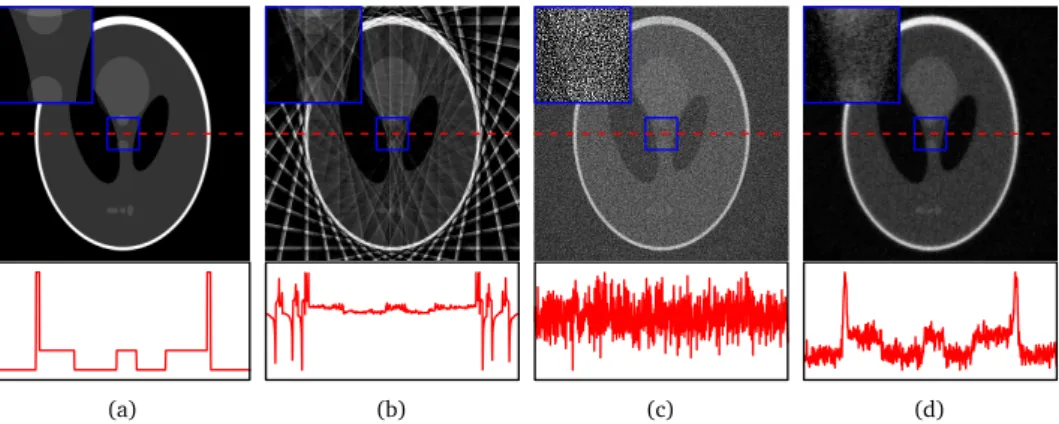
Figure 1.4: Three reconstructions of the Shepp-Logan head phantom (a), showing artifacts that occur with imperfect data. In (b) and (c), FBP was used to reconstruct the images. In (b), data from only 16 projections were used, and severe streak artifacts are present in the result. In (c), data from 1024 projections were used, but a large amount of Poisson noise was present, resulting in severe noise in the resulting image. In (d), SIRT, an algebraic method, was used to reconstruct the image using the same noisy projection data as in (c). The algebraic reconstruction image (d) has less noise compared to the FBP reconstruction (c). Under each image the line profile of the middle row is shown, and a small section is shown enlarged in the upper left of each image.

Algebraic reconstruction

Algebraic reconstruction methods are based on the discrete matrix representation of the tomographic reconstruction problem (Eq. (1.3)). Specifically, the reconstruction problem is written as a system of linear equations, which is then solved by an optimiza-tion method. Most algebraic methods minimize the difference between the forward projection of the reconstructed image with the acquired projection data, which is called

theprojection error. A popular choice is to minimize the`₂-norm of the projection

error, in which case we can write the algebraic approach as the following optimization problem:

xalg=argmin

x∈RN2

kp−W xk2 (1.9)

Because of the size of the matrixW, it is often impossible to use direct methods such as singular value decomposition to find a solution to Eq. (1.9). Instead, methods are used in which the projection error is iteratively minimized. Different mathematical optimization methods can be used to minimize the projection error, leading to different algebraic reconstruction methods. For example, if the projection error is minimized by Landweber iteration[Lan51], i.e. using gradient-descent steps on the projection error, the result is the Simultaneous Iterative Reconstruction Technique (SIRT). Iterations of the SIRT method can be written as:

xk+1₌_xk₊_α_WT _p

−W xk _(1.10)

Here,α∈Ris a parameter that influences the convergence rate and stability of the

(14)

the projection error is minimized by a Conjugate Gradient method[HS52], and the Algebraic Reconstruction Technique (ART)[GBH70], where the error is minimized by the Kaczmarz method[Kac37].

Since algebraic methods use a model of the tomographic reconstruction problem that includes only the projections that are actually acquired instead of assuming that an infinite number of projections are available, they tend to handle problems with a limited number of projections better than analytical methods. Furthermore, the effect of noise in the projection data can be limited in most algebraic methods by stopping the iteration process early, which is a form of implicit regularization. A comparison between a reconstruction computed by the algebraic SIRT method with a reconstruction computed by the analytical FBP method is shown in Fig. 1.4. Note that the artifacts caused by the noise are significantly reduced in the algebraic reconstruction, shown in Fig. 1.4d, compared to the analytical reconstruction, shown in Fig. 1.4c.

One of the main disadvantages of algebraic methods is their high computational costs. Several tens or hundreds of iterations are typically needed in algebraic methods to converge to an acceptable reconstruction image, with multiple projection operations per iteration. For the large datasets that are routinely acquired at experimental facilities, the high computational costs can be prohibitive in practice. For example, suppose we want to reconstruct a 10243_{3D volume using 1024 projections of 1024}_×_{1024 pixels}

each, which would be a medium-sized problem in synchrotron tomography. Using a state-of-the-art GPU system, it would take around 80 seconds to reconstruct the full volume with the analytical FBP method, while reconstructing with 200 iterations of the algebraic SIRT method would take around one and a half hours. Since a single tomographic dataset can often be acquired in a few minutes or less, the reconstruction time of algebraic methods tends too be too long to routinely use them in practice, and FBP is used instead.

In advanced tomographic experiments, one is often restricted to acquiring only a very limited number of projections, and a large amount of noise can be present in each projection. In these cases, algebraic methods are often also unable to produce reconstructions that are sufficiently accurate for further analysis, similar to analytical methods. The reason for this is that the linear system that is solved in algebraic methods (Eq. (1.9)) is highly underdetermined if N_θN_d N2. The result is that there exist

infinitely many reconstructions that have the same projection error, most of which are not suitable for analysis. It depends on the specific optimization method that is used which reconstruction is computed by an algebraic method. Furthermore, the projection matrixWis ill-conditioned in most applications of tomography. This means that even minor inconsistencies in the projection data, such as noise, can have a large effect on the reconstructed image.

The reconstruction quality of algebraic methods can be improved by exploiting prior knowledge about the scanned object or scanning system. Mathematically, this prior knowledge is often encoded as an additional term g:RN2→Rin the objective

function that is minimized, resulting inregularized iterative methods:

xreg=argmin

x∈RN2

kp−W xk2+λg(x)

(15)

(a) (b) (c) (d)

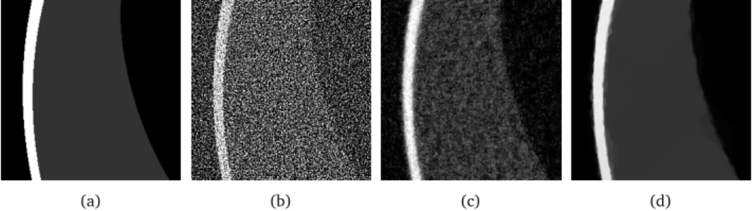
Figure 1.5: Zoomed-in reconstructions of the Shepp-Logan head phantom (a), showing the resulting images of three different reconstruction methods: (b) FBP, (c) SIRT, and (d) total variation minimization. The images were reconstructed on a 1024×1024 pixel grid, using projection data acquired withNd=1024

detectors andN_θ=256 projection angles, equally distributed in the interval[0,π], and additional Poisson noise applied.

Here, g(x)is a penalty function that penalizes undesired solutions that do not fit with the assumed prior knowledge, and the_λterm controls how strongly the penalty function is weighted compared to the projection error term. For example, when it is assumed that the gradient of the reconstructed object is sparse, a popular choice is to useTotal Variation minimization(TV-minimization) by setting g(x) =k∇xk1,

where∇is a discrete gradient operator[SP08]. If the assumed prior knowledge prior

knowledge is appropriate for the acquired data, regularized iterative methods can be extremely successful in reconstructing objects from (highly) limited data[BS11; Kos+13]. A comparison between FBP, SIRT, and TV-minimization reconstructions is shown in Fig. 1.5 for noisy projection data. A major disadvantage of regularized iterative methods is their high computational costs, which tend to be even higher than those of algebraic methods. For example, when reconstructing the 10243_volume

defined above on the same state-of-the-art GPU system, it would take more than aday

to reconstruct the full volume using the FISTA method for TV-minimization[BT09a].

1.3 Overview of this thesis

As explained above, in many applications of tomography, analytical methods produce reconstructions that are not accurate enough for further analysis. More accurate reconstructions can be obtained by using (regularized) iterative methods, but these can have computational costs that are too high to be used in practice. In this thesis, new reconstruction methods are developed that combine the analytical and algebraic approaches, resulting in methods that are as computationally efficient as analytical methods, but with a reconstruction accuracy of algebraic methods. Analytical methods allow for changing the filterhwithout increasing the needed computation time. We will use this freedom in filter choice to develop newfilter-basedreconstruction methods,

(16)

1.3. OVERVIEW OF THIS THESIS 9

introduced in this thesis, and reconstruction results are compared with other popular methods. In the rest of this section, the contributions and results of each chapter are explained.

In Chapter 2, the MR-FBP method is introduced, which uses a filter that minimizes the projection error of the resulting FBP reconstruction. The filter can be computed using an approach that is similar to algebraic reconstruction methods, i.e. minimizing the`2-norm of the projection error:

h∗=argmin

h∈RNd

kp−WFBP_h(p)k2 (1.12)

Note that the filter that is computed depends on the acquired data. The results of Chapter 2 show that the method is able to produce reconstructions with similar reconstruction quality as the algebraic SIRT method, but is much faster at producing them. Furthermore, it is shown that some forms of prior knowledge can be exploited to improve reconstruction quality, and that the computed filters automatically adapt to the characteristics of the object and the scanning parameters.

A different approach is taken in Chapter 3, where the SIRT-FBP method is introduced. This method explicitly approximates the SIRT method by the FBP method with a specific filter. The approximation is achieved by first rewriting the SIRT method into a matrix form, and then approximatingkiterations of SIRT by a single convolution operation. By

comparing with the standard FBP method, it is possible to show that the approximated SIRT method is identical to the FBP method with a specific angle-dependent filter. The filter can be pre-computed for a certain scanning geometry by a single SIRT-like iteration method, after which it can be reused for datasets that are acquired with the same geometry. The results of Chapter 3 show that reconstructions computed with the SIRT-FBP method are virtually identical to standard SIRT reconstructions.

In Chapter 4, a method is introduced that allows one to approximate a slow regu-larized iterative method inside a (small) subvolume of the complete reconstruction volume. If one is only interested in a small subvolume of the scanned object, as is often the case, this method can significantly reduce the computation time that is needed to perform the required analyses. Note that regularized iterative methods generally need to compute the entire reconstruction volume, since they are based on minimizing a global objective function (Eq. (1.11)). The local approximation method is based on extending the SIRT-FBP method introduced in Chapter 3 to allow for different types of additional regularization terms. In the results of Chapter 4, we show that the reconstruction quality of the local approximations is almost identical to that of the much slower global regularized iterative methods for several popular types of prior knowledge, such as TV-minimization.

The NN-FBP method is introduced in Chapter 5. An NN-FBP reconstruction consists of a nonlinear combination of multiple FBP reconstructions, each with a different filter. The filters are pre-computed by using projection data and high-quality reconstructions of objects that are similar to the objects that will be reconstructed later. Methods from neural network theory are used totrainthe filters, after which they can be used to

(17)

reconstructions with a significantly higher quality than both analytical and algebraic reconstruction methods. Also, it is shown that the method can be used to approximate slow regularized iterative methods in the case that it is not possible to acquire a large number of projections for use in training.

An application of the NN-FBP method in electron tomography is presented in Chapter 6. In electron tomography, acquiring a large number of projections is both time-consuming and labor-intensive. As a result, it is difficult to scan a large number of samples and obtain statistically significant results for certain sample characteristics. By lowering the number of projections that need to be acquired, the effort needed to obtain statistically significant results can be reduced. In Chapter 6, we use the NN-FBP method to obtain accurate reconstructions of gold nanoparticles using a very limited number of projections. The NN-FBP method is trained on a small number of nanoparticles that are scanned with a higher number of projections. Results show that the NN-FBP method is able to produce accurate reconstructions with only a few projections, and that the method can be used to obtain statistically significant results with reduced scanning time.

(18)

2

Data-dependent filtering

2.1 Introduction

Tomographic reconstruction problems are found in many applications, such as X-ray scanners in medical imaging, or electron microscopy in materials science[Gra13]. In the standard tomographic problem, we aim to reconstruct an object from its projections, acquired for a range of angles. This problem has been studied extensively because of its practical relevance, leading to a wide range of reconstruction methods. For an overview of previous work, see[KS01; Nat01; Buz08]. Most of the current reconstruction methods can be separated into two groups:analyticalmethods andalgebraicmethods.

The basis of analytical reconstruction methods is a continuous representation of the tomographic problem. This continuous model is inverted, and the result is discretized. The resulting reconstruction methods, of which the filtered backprojection (FBP) method is the most widely used, are usually computationally efficient. Furthermore, if projection data of sufficiently high quality is available, reconstructions computed by these methods are often accurate. These two properties are among the reasons that the FBP method is very popular in practice_[PSV09_], along with its ease of implementation. An important drawback of analytical methods is that they are based on an approximation of a model where perfect data is available forallprojection angles. If the available

data is not perfect, either because few projections are available or because the data is noisy, the quality of analytical reconstructions will suffer from interpolation effects.

Practical considerations can lead to limited or noisy projection data in many ap-plications of tomography. In electron tomography, for example, the electron beam

This chapter is based on:

D. M. Pelt and K. J. Batenburg. “Improving Filtered Backprojection Reconstruction by Data-Dependent Filtering”.IEEE Transactions on Image Processing23.11 (2014), pp. 4750–4762.

(19)

damages the sample, leading to a hard limit on the number of projections that can be measured[MDG95]. In many other applications, there is a limit on the duration of a single scan. To decrease the scan duration, one can either acquire fewer projec-tions or use a reduced dose per projection. In industrial tomography, process speed considerations limit the duration of each scan[Sip93].

Algebraic methods are based on a discrete representation of the tomographic problem, leading to a linear system of equations. This system is solved to obtain a reconstructed image. Since algebraic methods use a model of the actual data that is available, they usually yield more accurate reconstructions from limited data than analytical methods. Furthermore, by using specific ways of solving the linear system, it is possible to reduce the effect of noise on the reconstruction. An important drawback of algebraic methods is that they are computationally more expensive than analytical methods. The linear system that has to be solved is usually very large, and the iterative methods that are used often need a large number of iterations to converge to an acceptable solution.

In many applications of computed tomography, the computational efficiency of a reconstruction method is an important consideration. For example, in fast x-ray micro-tomographic experiments at synchrotrons, the speed of the post-processing pipeline has to match the high speed of data acquisition_[Mok₊13_]. In fact, the computation efficiency of the FBP method is an important reason for why it is still commonly used instead of more advanced reconstruction methods[PSV09].

Methods that reduce the computation time of algebraic methods have been proposed by other authors. One approach is to implement algebraic methods more efficiently by using graphic processing units (GPUs)[XM05; Pan+11]. Other approaches focused on improving the convergence of algebraic methods, for example by improving the properties of the linear system [GB08]. Although these improvements reduce the computation time of algebraic methods significantly, even faster methods can be obtained by changing the algebraic methods themselves.

One such approach is taken in [BP12], where an angle-dependent FBP filter is calculated, such that the resulting FBP method approximates an algebraic method. Although the resulting method is able to approximate the algebraic method well, calculating the filter requires a large number of runs of the algebraic method, which is computationally expensive. The resulting filter can be reused for problems with identical projection geometry, but a change in geometry requires calculation of a new filter.

A filter that approximates an algebraic method is also derived in[Zen12], in which a reformulation of the SIRT algebraic method is translated to a fixed filter for the FBP method. An extension of the method for noisy projection data is given in[ZZ13]. The derived filter does not depend on the scanning geometry of the problem, and during derivation it is assumed that enough projections are available such that certain approximations are accurate. As such, the resulting method has more in common with analytical reconstruction methods than with algebraic methods.

A different approach, specific to tomosynthesis, is proposed in[Nie+12]. Instead of calculating a reconstruction image directly, Nielsen et al. calculate a filtermatrix,

(20)

2.2. NOTATION AND CONCEPTS 13

the final reconstruction. Nielsen et al. show that their filter matrix can be formed efficiently in the case of tomosynthesis, but a complex method is needed to obtain this efficiency. Similar to[BP12], a change in geometry requires calculation of a new filter. Other methods for tomosynthesis use algebraic reconstructions of certain test objects to create filters[Kun+07; Lud+08].

In this chapter, we introduce a new reconstruction method, theminimum residual

filtered backprojectionmethod (MR-FBP), that combines ideas from both the analytical

and algebraic approach, resulting in a method with a data-dependent filter. The method is based on an algebraic model of the tomographic problem, resulting in a method that can reconstruct problems with limited data more accurately than analytical methods. The linear system that has to be minimized, however, is based on filtered backprojection. Therefore, the system is much smaller than the ones used in algebraic methods or other approaches, making the method computationally efficient. Furthermore, we are able to use filtered backprojection to form our linear system, leading to a simple and efficient implementation.

This chapter is structured as follows. We formally define the tomographic recon-struction problem and analytical and algebraic reconrecon-struction methods in Section 2.2. In Section 2.3, we introduce and explain the key contribution of this chapter: the minimum residual filtered backprojection method. Considerations concerning its im-plementation are discussed in Section 2.4. An extension of the method is given in Section 2.5, where additional constraints are added to its linear system to improve reconstruction quality. The experiments we performed to test the new method are explained in Section 2.6. Results, where we compare MR-FBP with popular reconstruc-tion methods, are given in Secreconstruc-tion 2.7, along with a discussion on the interpretareconstruc-tion of the results. Finally, we conclude the chapter in Section 2.8, where we give a summary and some final remarks.

2.2 Notation and concepts

In this section, we will explain the mathematical notation used throughout the chapter, and introduce all relevant concepts. We begin by formally defining the tomographic reconstruction problem. Filtered backprojection and algebraic methods are explained, and their mathematical definitions are given.

Problem definition

We consider the problem of reconstructing a two-dimensional object from its parallel-beam projections, with a single rotation axis. The approach we introduce here can be adapted to other geometries as well, such as fan-beam or cone-beam projections. The unknown object is modeled as a finite and integrable two-dimensional function

f :R2→Rwith bounded support.

(21)

Figure 2.1: The two-dimensional tomography model used in this chapter. Parallel lines, rotated by angleθ, pass through the objectf. A linelθ,thas the characteristic equationt=xcosθ+ysinθ, and a projection

P_θ(t)off is given by the line integral off over the linel_θ,t.

P_θ(t)of f over a single linel_θ_,t is given by: P_θ(t) =

Z

lθ,t

f(x,y)ds (2.1)

=

Z Z

R2

f(x,y)δ(xcosθ+ysinθ−t)dxdy (2.2)

Thetomographic reconstruction problemis concerned with the reconstruction of the

unknown object f from its measured projectionsP_θ(t)for different combinations ofθ

andt. This projection geometry is shown graphically in Fig. 2.1.

In practice, only a finite set of projectionsP_θare measured, one for each combination

of projection angle_θ ∈Θ ={θ0,θ1, . . . ,θN_θ−1} and detectork ∈ {0, 1, . . . ,Nd−1}, whereN_θis the number of projection angles, andNd the number of detectors. Relative to the central detector, the position of a detectorkis given byτk:

τk=s

k−Nd₂−1

, (2.3)

where sis the width of a detector. The entire set of measured detector positions is

given byT={τ0,τ1, . . . ,τNd−1}. Using the measured projection data, the unknown object is reconstructed on anN_×N grid of square pixels. We assume, without loss of

generality, that the width of each pixel is equal to 1. Often, the number of pixels in each row of the reconstruction grid is taken equal to the number of detectors.

Filtered backprojection

One approach to solving the tomographic reconstruction problem is to take Eq. (2.2), and try to find an expression for f(x,y)from this equation. Thefiltered backprojection

(22)

2.2. NOTATION AND CONCEPTS 15

Figure 2.2: The Ram-Lak (ramp) filter for the FBP method, in real space. This filter is a discrete approximation of the optimal filter.

with a filterh:R→R:

q_θ(t) =

Z ∞

−∞

h(τ)P_θ(t₋τ)dτ (2.4)

This convolution can be also be performed in Fourier space, where ˆPand ˆhdenote the

Fourier transforms ofPandhrespectively:

q_θ(t) =

Z ∞

−∞

ˆ

h(u)ˆP_θ(u)e2πıutdu (2.5)

One can show[KS01]that we obtain an expression for f(x,y)if we take ˆh(u) =_|u_|:

f(x,y) =

Z π

0

q_θ(xcosθ+ysinθ)dθ (2.6)

In practice, it is not possible to use Eq. (2.6) to reconstruct the object, since it requires P_θ(t)to be known forallanglesθ ∈[0,π)and t ∈R. Instead, we only

know P_θ(t)for the measured anglesΘand detector positionsT. To be able to use

these discrete measurements, Eq. (2.6) has to be discretized, after which the filtered backprojection method is obtained:

f(x,y)≈FBPh(x,y) = X

θd∈Θ X

τp∈T

h(τp)Pθd(t−τp) (2.7) wheret=xcosθd+ysinθd. Sincet−τpis usually not equal to one of the measured detector positions, some interpolation is needed to find the value ofP_θ

d(t−τp). Linear interpolation is often used, since projection data is usually reasonably smooth.

The filterhis only needed for discrete positionsτ_p_∈T, and is therefore usually

spec-ified as a vectorh. Several discrete approximations of the optimal filter ˆh(u) =|u|are

used in practice, such as the Ram-Lak (ramp), Shepp-Logan, and Hann filters[Far+97; WWH05]. One of the most popular filters is the Ram-Lak filter, where we take the optimal ˆh(u) =_|u_|, and set ˆh(u) =0 whenu>u_c for someu_c. This filter is shown, in

real space, in Fig. 2.2.

(23)

Figure 2.3: Three reconstructions of the Shepp-Logan head phantom (a), showing artifacts that occur with imperfect data. In (b) and (c), FBP was used to reconstruct the images. In (b), data from only 16 projections were used, and severe streak artifacts are present in the result. In (c), data from 1024 projections were used, but a large amount of Poisson noise was present, resulting in severe noise in the resulting image. In (d), SIRT, an algebraic method, was used to reconstruct the image using the same noisy projection data as in (c). The algebraic reconstruction image (d) has less noise compared to the FBP reconstruction (c).

backprojected to obtain the reconstructed image. One of the advantages of FBP is that it is fast compared to other methods: the filtering step can be performed efficiently in Fourier space inO(N_θNdlogNd)time, and only one backprojection is needed, which can be performed inO(N_θN2)time.

The quality of an FBP reconstruction depends on how well the discretized equation Eq. (2.7) approximates the continuous equation Eq. (2.6). If data for many projection angles (say, several hundred) are known, an FBP reconstruction is often highly accu-rate. However, when the number of projections is small compared to the size of the image, the approximation is not very accurate, and severe artifacts can appear in the reconstructed image. Furthermore, noise in the projection data can cause artifacts in the reconstruction as well. FBP with the Ram-Lak filter is especially sensitive to noise, since high-frequency components of the projection data are amplified by the filter. The artifacts can make subsequent analysis of the reconstruction very difficult. Examples of artifacts in FBP reconstructions of imperfect data are shown in Fig. 2.3.

Algebraic methods

A different approach to solving the tomographic problem is to use a discrete represen-tation of the problem. Here, we represent the discrete projection data as a single vector p ∈RNθNd, and represent the unknown image as a vector _x ∈_RN2. The_projection matrixWhasN_θNdrows andN2columns, with elementwi jspecifying the contribution of pixel jto detectori. We refer to the product ofW with an imagex as theforward projectionofx. Similarly, the product ofWTwith projection datapis referred to as the

backprojectionofp. If we look at the definition of the discrete FBP method (Eq. (2.7)),

we see that the backprojection in the FBP method is identical to multiplication of the filtered sinogram withWT_.

(24)

2.3. MINIMUM RESIDUAL FILTERED BACKPROJECTION 17

solution imagexalgis defined as:

xalg=argmin

x k

p−W xk22 (2.8)

The algebraic solutionxalgcan be found by solving the linear systemW x=pin a least squares sense.

The algebraic linear system is typically too large to be solved directly. Therefore, an iterative optimization method is normally used, which can often exploit the sparse structure of the projection matrix to improve computational and memory requirements. Different iterative methods can be used, leading to various algebraic reconstruction methods. One example is SIRT[KS01], belonging to the class of Landweber iteration methods [Lan51], which uses a specific Krylov subspace method to minimize the projection error. A different method is CGLS[Bjö96], which uses a conjugate gradient method.

The advantage of using an algebraic method compared to analytical methods is that the projection matrixW can be adapted to the actual geometry that was used during scanning. Therefore, these methods use a model of the actual data that is available, instead of assuming perfect data, as in analytical methods. Another advantage of algebraic methods is that additional constraints can be imposed on the reconstructed imagex, which can be used to improve reconstructions by exploiting prior knowledge. For example, total variation minimization based methods use algebraic methods to minimize the projection error, with an additional constraint that the`1-norm of the

gradient ofx should be minimal as well[SP08].

The main disadvantage of algebraic methods compared to analytical methods is their computation time. Because of the large system size, and the number of iterations that are needed to solve them, the time to reconstruct an image using an algebraic method is often several orders of magnitude larger than filtered backprojection, even when optimized for graphic processor units (GPUs)[XM05]. In the next section, we introduce a new reconstruction method that uses ideas from algebraic methods to improve filtered backprojection, leading to a method that is both fast and accurate.

2.3 Minimum residual filtered backprojection

We will now present the key contribution of this chapter: the minimum residual filtered backprojection method (MR-FBP). We start by noting that the FBP method is a linear operation on the projection data. In other words, the operation of the FBP algorithm can be modeled as a linear operatorM :RNdNθ _→_RN2applied to the projection data p, which can be written as aN2×NdNθmatrixMh:

FBP_h(p) =Mhp (2.9)

As explained in Section 2.2, FBP consists of a convolution ofp with filterh, followed by a backprojection of the result:

(25)

whereC_hpis the convolution ofpbyh, specified by theNdNθ×NdNθmatrixCh.

One of the properties of a convolution of two vectors is that it iscommutative.

Therefore, we can exchange the positions ofhandpin Eq. (2.10):

M_hp=WT_C

ph (2.11)

Up to this point, we have only rewritten the equation of the FBP method. Now, we will improve the method by changing the filterhfrom one of the standard filters to one specific to the problem we are solving. To calculate the specific data-dependent filterh∗, we minimize the squared difference of the projections of the reconstruction with the measured projection data, similar to algebraic methods:

h∗=argmin

h k

p−W FBP_h(p)k22 (2.12)

Using Eqs. (2.9) and (2.11), we can write this as:

h∗=argmin

h

p−W WTC_ph

2

2 (2.13)

As with the algebraic methods, we can findh∗by solving the following linear system forhin the least squares sense:

Aph=p (2.14)

whereA_p₌W WT_C

p.

After computing the least squares solution h∗ to the linear system of Eq. (2.14), the MR-FBP reconstruction is obtained by computing the FBP reconstruction withh∗ as filter. The complete MR-FBP algorithm is given by:

Algorithm 2.1MR-FBP reconstruction method

1. CalculateA_p=W WT_C

p.

2. Find least squares solutionh∗ofA_ph=p.

3. ReturnFBP_h∗(p)as MR-FBP reconstruction.

The linear system we need to solve in step 2) looks similar to the systemW x=p, which is solved in the least squares sense by algebraic methods (Eq. (2.8)). The difference is that the system of Eq. (2.14) has fewer unknowns:AphasNd columns if we impose thathis angle-independent, whileW hasN2columns. As we will show

in Section 2.4, we are able to reduce the number of columns ofA_p toO(logNd)by exponential binning, without reducing the reconstruction quality significantly.

(26)

2.4. IMPLEMENTATION 19

2.4 Implementation

Although the number of unknowns of the MR-FBP method is smaller than that of algebraic methods, the actual implementation of the method is important to actually obtain a method that is computationally more efficient. In this section, we give details on how we implemented the MR-FBP method in this chapter to obtain the experimental results of Section 2.7. We will begin by discussing how the matrixA_p of Eq. (2.14) can be calculated efficiently. Furthermore, we will show that the size of the linear system can be reduced by exponential binning. Finally, we discuss the computational complexity of the MR-FBP method compared to existing methods.

Calculation of

A

_p

The first step of the MR-FBP method is to calculate the matrixAp=W WTCp. Usually,

the projection matrix W is not used directly by algebraic methods, since it can be very large. Instead, multiplication ofW with an imagex is calculated implicitly by calculating the line integrals ofx on-the-fly_[PBS11_]. Similarly, multiplication ofWT with a sinogrampis calculated by backprojectingp on-the-fly. Here, we use a similar approach to calculateA_p, column by column.

Denoting a column jofA_pbyA_p₍:,j), we have:

Ap(:,j) =Apej (2.15)

whereejis a unit vector with all elements zero except for element j, which is equal to one. Using the definition ofAp, we see that:

Ap(:,j) =W WTCpej=W W T

Cejp=W FBPej(p) (2.16)

In other words, we can calculate a column jofA_pby creating a filtered backprojection reconstruction with filterej, and forward projecting the result. By doing this for every column, we can calculate matrixA_p.

Exponential binning

At this point, the MR-FBP linear system of Eq. (2.14) has NdNθ equations andNd unknowns, one for each detector element. Although the system is smaller than the one used in algebraic reconstruction methods, which haveN_dN_θ equations andN2

unknowns, we can further reduce the number of unknowns byexponential binning.

Exponential binning was also used successfully to reduce system sizes in[BK06]and Chapter 5 of this thesis.

In exponential binning, we assume that the filterhis a piecewise constant function ofN_bpieces. Each constant region of the function is called abin, and the boundary

points of a binβiare defined by positionssi andsi+1:βi= (si,si+1). The width of a bin is equal to the difference between its boundary pointsd_i =s_i₊₁−s_i. Since the

(27)

Figure 2.4: A filter with exponential binning, where we impose that the filter is symmetrical, and consists of several bins with a constant filter value. The size of the bins increases exponentially away from the center of the filter.

one element for each bin. The idea of exponential binning in the MR-FBP method is that we can reduce the number of unknowns of the linear system fromN_d toN_b, by

using fewer bins than detectors (N_b<N_d). The question remains how to choose the

boundary points of the bins.

Looking at Fig. 2.2, we see that the Ram-Lak filter has most details aroundn=0,

and drops to zero relatively quickly for|n_{|→ ∞}. This suggests that we should use

small bins aroundn=0, and can use larger bins further away from the center. In

this chapter, we use bins with widths that increase exponentially away fromn=0.

Specifically, we taked_i=1 for_|i_|<N_l andd_i=2|i|−Nl for_|_i_|≥_N

l, withβ0being the central bin. The number of bins with width 1 is specified byN_l, where larger values

lead to more detail around the center of the filter, but more unknowns as well. For the rest of this chapter, we usedNl=2, unless specified otherwise. We can reduce the number of bins even more by making it symmetric, defining new binsB₀=β₀and Bi = (βi∪β−i)for i6=0. A filter with exponential binning andNl=2 is shown in Fig. 2.4.

Since the bin width increases exponentially, we end up withO(logN_d)bins.

There-fore, by using exponential binning, we have reduced the number of unknowns of the MR-FBP method fromNd toO(logNd). The restrictions we impose on the filter by assuming it is piecewise constant and symmetrical can reduce the quality of the MR-FBP reconstructions. We will show in Section 2.7, however, that the quality does not decrease significantly by using exponential binning, while the time it takes to calculate the reconstructions greatly decreases.

The matrixApwith an exponentially binned filter can again be calculated column

by column. In order to do this, we change the filterejof Eq. (2.16) to a vectorqBi, in which each filter element included in binB_iis set to one, and all other elements are

(28)

2.5. ADDITIONAL CONSTRAINTS 21

Computational complexity

For many tomographic reconstruction methods, the most costly subroutines com-putationally are forward projecting and backprojecting, for which straightforward implementations takeO(NdNθN)andO(NθN2)time, respectively, although faster

im-plementations exist which use hierarchical decomposition[BB00]. We can compare the computational costs of different reconstruction methods by comparing the number of projection operations each method has to perform. Filtered backprojection consists of a single projection operation: the final backprojection of the filtered sinogram. Algebraic methods usually perform a few projection operations per iteration. The SIRT method, for example, performs two projection operations per iteration, and typically has to performO(Nd)iterations to converge to an acceptable solution.

The MR-FBP method has to perform one forward projection and one backprojection for every column ofApduring its calculation. Because there areO(logNd)unknowns, MR-FBP has to performO(logN_d)projections. The total computation time of calculating

ApbecomesO (NθNdN+NθN2)logNd

. If we assume thatN_d_≈N, which is often the

case, the total computation time becomesO N_θN_d2logNd

_{. To summarize, FBP, SIRT,} and MR-FBP have to performO(1₎,O(Nd), andO(logNd)projections, respectively, which shows that MR-FBP has to perform significantly fewer operations than SIRT.

Of course, the MR-FBP method also has to find the least squares solution to its linear system of Eq. (2.14). Because of its smaller size however, we can use direct methods to find this solution, instead of the iterative methods used in algebraic methods. The direct method we used in this chapter to generate the results of Section 2.7, the_gels* lapack routine, uses singular value decomposition, and can solve anm×nsystem in

O(mn2)time. Since the MR-FBP system hasNdNθ equations and logNd unknowns, the least squares filterh∗can be found inO(NdNθ[logNd]2)time. Summing both the calculation ofA_pand ofh∗, the total computation time of the MR-FBP method becomes

O N_θN2logN_d+N_dN_θ[logN_d]2.

2.5 Additional constraints

The reconstruction quality of algebraic reconstruction methods can be improved by exploiting prior knowledge about the object that was scanned. One approach of exploiting this knowledge is to add an additional constraint to the system that is minimized. Formally, such a reconstructionx∗can be found by solving the following equation:

x∗=argmin

x

kp−W xk22+λg(x)

(2.17)

whereg(x)is a function depending on the type of prior knowledge that is exploited. For example, if one knows that the object that is reconstructed has a sparse gradient, total-variation minimization can be used by settingg(x) =k∇xk1[SP08]. The parameterλ

(29)

A similar approach can be applied to the MR-FBP method, by imposing an additional constraint on the optimal filterh∗:

h∗=argmin

h

p−W WTC_ph

2

2+λg(h)

(2.18)

Different functionsf can be used to exploit various kinds of prior knowledge. In this

chapter, we will use one example, where the change in intensity of the reconstructed image in the horizontal direction and vertical direction is minimized. This can be achieved by lettingg(h) =k∇xWTCphk2+k∇yWTCphk2, where∇xf denotes the horizontal gradient of image f, and∇yf the vertical gradient. The horizontal and vertical gradient can be approximated by the linear Sobel operatorsDx andDy, which convolve the image with two-dimensional kernelsGxandGy, respectively:

Gx= 



+1 0 −1

+2 0 −2

+1 0 −1



,Gy=





+1 +2 +1

0 0 0

−1 −2 −1



 (2.19)

If we approximate the gradients byDx andDy, we can add the additional constraints to the linear MR-FBP system, as additional equations:





W WT_C

p

λDxWTCp

λDyWTCp



h=

  p 0 0   (2.20)

The least squares solutionh∗_GMof this system can be found using standard methods, by solving:

(2.21) h∗_GM=argmin

h

p−W WTC_ph

2 2+λ

D_xWTC_ph

2 2+

D_yWTC_ph

2 2

The resulting method, which we call MR-FBPGM, finds a filter that minimizes a weighted

sum of the residual and the horizontal and vertical gradient of the resulting reconstruc-tion. The method can improve reconstructions of objects that have a small gradient. In the case of noise in the projection data, MR-FBP_GMcan improve reconstructions as well, since the gradient of the object is usually much smaller than that of image noise. Therefore, by reducing the gradient of the reconstructed image, we reduce the amount of image noise as well.

Similar to the MR-FBP method, we can calculate the matrixA_pof the MR-FBP_GM method column by column. For a column j, we can calculate the FBP reconstruction

with filter ej. We can then forward project this reconstruction to obtain the top part of column j of the linear system shown in Eq. (2.20). The remaining part of

column jcan be calculated by applying the Sobel operatorsDx andDy to the FBP reconstruction. Since the gradient image calculations can be performed efficiently in Fourier space, the asymptotic computational complexity of theApcalculation step

(30)

2.6. EXPERIMENTS 23

(a)PHANTOM1 (b)PHANTOM2 (c)PHANTOM3

Figure 2.5: The three phantom images used in this chapter.PHANTOM1 is the Shepp-Logan head phantom,

PHANTOM2 represents a cross section of an engine block, andPHANTOM3 is a difficult to reconstruct object

with both discrete and continuous areas.

O((NdNθ+N2)[logNd]2)time, which is a slightly higher complexity than MR-FBP without gradient minimization. The total computational complexity of MR-FBPGMis

equal toO N_θN2logNd+ (NdNθ+N2)[logNd]2

.

2.6 Experiments

To compare the performance of the MR-FBP and MR-FBP_GM methods with other methods, we implemented them using Python 2.7.3, PyCUDA 2012.1, and Numpy 1.6.3[Oli07]built with ATLAS 3.10.0[WP05]. The GPU implementations of the for-ward and backprojection operations are based on the ASTRA-Toolbox[PBS11], in which backprojection is not the exact transpose of forward projection for performance reasons. We applied MR-FBP on three phantom images and two experimentalµ-CT datasets, comparing the results of MR-FBP with SIRT, an algebraic method, and FBP with three different standard filters: the Ram-Lak filter, the Hann filter, and the Shepp-Logan filter. We compare MR-FBPGMreconstructions with MR-FBP, FBP, and SIRT reconstructions of

one of the three phantoms, with noise in the projection data.

The three phantom images are shown in Fig. 2.5. Each phantom image is repre-sented on a 4096×4096 pixel grid, on which projections are calculated. Afterwards,

the projection data is rebinned to 1024 detector elements, and all reconstructions are calculated on a 1024×1024 pixel grid. We calculate reconstructions for varying

numbers of projection angles, and compare them to the original phantom image, scaled to a 1024×1024 pixel grid by averaging 4×4 squares.

(31)

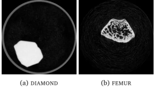
(a)DIAMOND (b)FEMUR

Figure 2.6: Reconstructions of theµCT datasets used in this chapter. The reconstructions were calculated using SIRT and all available projections.

For each experiment, we report the mean absolute error and structural similar-ity (SSIM) index [Wan+04]of reconstructions of the various methods. The mean absolute error is defined as:

ep(x,o) = N_D−1P

i∈D|xi−oi|

maxo−mino (2.22)

wherex ∈RN

2

is the reconstructed image,o∈RN

2

the correct image, and the average is taken over allN_Dpixels within the central discDof radiusN/2. For the experimental

data, the mean absolute errors and SSIM indices are calculated with respect to SIRT reconstructions from projection data of all available projections, shown in Fig. 2.6. The SSIM index measures the similarity between two images, and was designed to represent human visual perception more accurately than other metrics. A higher SSIM index corresponds with larger perceptual similarity between the compared images. For the phantom experiments, we also report the mean absolute residual, defined as:

er(x,p) = (NdNθ)−1

NdNθ−1 X

i=0

(W x)_i−p_i

(2.23)

where x ∈RN2 is the reconstructed image, and p∈RNθNd the measured projection data.

2.7 Results and discussion

Results for simulation phantoms

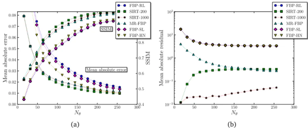
The mean absolute error, SSIM index, and mean absolute residual forPHANTOM1 are shown in Fig. 2.7 as a function of the number of projection anglesN_θ. The results show

(32)

2.7. RESULTS AND DISCUSSION 25

0 50 100 150 200 250 300

Nθ

0.00 0.01 0.02 0.03 0.04 0.05 0.06 0.07 0.08

Mean

absolute

error

0.4 0.5 0.6 0.7 0.8 0.9 1.0

SSIM FBP-RL SIRT-200 SIRT-1000 MR-FBP FBP-SL FBP-HN

Mean absolute error SSIM

(a)

0 50 100 150 200 250 300

Nθ

10−2 10−1 100 101 102 Mean absolute residual FBP-RL SIRT-200 SIRT-1000 MR-FBP FBP-SL FBP-HN (b)

Figure 2.7: The mean absolute error, SSIM, and mean absolute residual of reconstructions calculated with different methods, forPHANTOM1. The methods shown are FBP with the Ram-Lak filter (FBP-RL), FBP with

the Shepp-Logan filter (FBP-SL), FBP with the Hann filter (FBP-HN), SIRT with 200 iterations (SIRT-200), SIRT with 1000 iterations (SIRT-1000), and the MR-FBP method (MR-FBP).

found for the SSIM, with significantly higher indices for SIRT and MR-FBP, compared to all tested FBP methods. Compared to SIRT, MR-FBP produces reconstructions with slightly higher errors, lower SSIM indices, and higher residuals. Later results in Fig. 2.9 will show, however, that MR-FBP is significantly faster than SIRT at producing these reconstructions. Results for the other two phantom images are similar to those of PHANTOM1.

For all three phantoms, reconstructions of FBP with the Ram-Lak filter, SIRT, and MR-FBP are shown in Fig. 2.8 for 32 projection angles. Note that in all comparison images in this chapter, the pixel value that a certain graylevel represents is identical for all compared methods. A zoomed inset is included in most images, giving a better indication than the entire image of how the reconstruction will look at full resolution. Figure 2.8 shows that both MR-FBP and SIRT are able to reduce the number of streak artifacts compared to standard FBP. Visually, the sharpness of the MR-FBP and SIRT reconstructions is slightly lower than that of the FBP reconstructions. In some applications, the higher sharpness of the FBP reconstructions might be preferable despite its artifacts, especially when the user is familiar with the scanned objects and FBP artifacts. In other applications, and in common post-processing steps such as segmentation, the artifacts present in FBP reconstructions can be problematic, and MR-FBP might be preferable.

The time it takes to calculate the reconstructions ofPHANTOM1 using the different methods is shown in Fig. 2.9. In Fig. 2.9a, the reconstruction time is shown as a function of the number of projections, for a fixed number of detectors N_d =1024.

The results show that MR-FBP is significantly faster than SIRT, but slower than FBP with a standard filter. Specifically, MR-FBP is around 20 times faster than SIRT with 200 iterations in these cases, which is expected since MR-FBP has to perform around 2 logN_d=20 forward projections and backprojections, while SIRT with 200 iterations

(33)

(a) FBP-RL (b) SIRT-200 (c) MR-FBP

(d) FBP-RL (e) SIRT-200 (f) MR-FBP

(g) FBP-RL (h) SIRT-200 (i) MR-FBP

Figure 2.8: Reconstructions of the phantom images, from data with 32 projections, for different reconstruction methods.

0 50 100 150 200 250 300

Nθ

10−3 10−2 10−1 100 101 102

Reconstruction

time

(

s

)

FBP-RL SIRT-200 SIRT-1000 MR-FBP

(a)

101 ₁₀2 ₁₀3 ₁₀4

N=Nd

10−4 10−3 10−2 10−1 100 101 102 103

Reconstruction

time

(

s

)

FBP-RL SIRT-200 SIRT-1000 MR-FBP

(b)

Figure 2.9: The reconstruction time of thePHANTOM1 image. In (a),N=Nd=1024, and the reconstruction

time is shown as a function of the number of projectionsNθ. In (b), the number of projections is 64, and the

(34)

2.7. RESULTS AND DISCUSSION 27

101 ₁₀2 ₁₀3 ₁₀4 ₁₀5 ₁₀6 ₁₀7

I0

0.0 0.1 0.2 0.3 0.4 0.5 0.6 0.7

Mean

absolute

error

0.1 0.2 0.3 0.4 0.5 0.6 0.7 0.8 0.9

SSIM FBP-RL SIRT-200 SIRT-1000 MR-FBP FBP-SL FBP-HN

Mean absolute error SSIM

Figure 2.10: Mean absolute error and SSIM of reconstructions ofPHANTOM1 from data of 64 projections with various amounts of Poisson noise applied.

time is shown as a function of the number of detectors, for a fixed number of projections

N_θ=64.

In Fig. 2.10, the mean absolute error of reconstructions ofPHANTOM1 with different methods is shown, for data of 64 projections with various amounts of Poisson noise applied. The parameterI₀indicates the amount of applied Poisson noise, with lower

values corresponding to higher amounts of noise. Specifically, noise was applied by first transforming the projection data to virtual photon counts, whereI₀corresponds

to the largest photon count of all detector elements. For each detector element, a new photon count is sampled from a Poisson distribution with the original photon count as expected value. The resulting noisy photon counts are transformed back to obtain noisy projection data.

Since the Ram-Lak filter amplifies high-frequency signals, the reconstructions of FBP with the Ram-Lak filter are of low quality when noise is present in the projection data. Other filters, like the Hann filter, suppress high-frequency signals, and therefore yield reconstructions of higher quality. Algebraic techniques, like SIRT, often include a form of regularization on the reconstruction image, yielding reconstructions of even higher quality when noise is present. The results of Fig. 2.10 show that, as expected, SIRT reconstructions have the lowest error and highest SSIM, while the FBP method with the Hann filter yields reconstructions with higher errors and lower SSIM, and FBP with the Ram-Lak filter produces reconstructions with the highest error and lowest SSIM. The MR-FBP method yields reconstructions with similar errors and SSIM indices to the SIRT method, for every noise level, but requires less computation time. Examples of reconstructions of data with two different noise levels are shown in Fig. 2.11, for FBP with the Ram-Lak filter, SIRT, and the MR-FBP method.