LAB 1 CLOUD CAPACITY PLANNING

Capacity Planning in Cloud Computing

Technology

The traditional notion of capacity planning changes when using cloud computing, there are two points of view to consider one from the user of cloud services and the other from the provider.

1 From the Cloud User’s Point of View

When services are executed on demand using cloud resources the burden of capacity planning shifts to the provider of the cloud services. However, cloud users have to be able to negotiate SLAs with cloud service providers. Since there may be SLAs for different QoS metrics, cloud users should consider using the notion of utility function to determine the combined usefulness of cloud services as a function of the various SLAs. Utility functions are used quite often in economics.

The following notation to formalize the problem of optimal selection of SLAs to be negotiated with the provider of cloud services. Let

SLAr – SLA (in seconds) on the average response time per transaction.

SLA_{x – SLA (in tps) on the transaction throughput.}

SLA_{a – SLA on the cloud availability.}

C_r

₍

₎

SLA is SLAr .

C_x

₍

₎

is SLAx .

C_a

₍

₎

Global utility – The global utility function is composed of terms that represent the utility for various metrics such as response time, throughput, and availability. The utility is a dimensionless number in the [0,1] range.

W

,W

,W

respectively, used to compute the global utility Wr+Wx+Wa=1 .

The cost functions used in the following example are:

C_r(SLA_r)=α_re−βrSLAr _{; (1)}

C_x(SLA_x)=α_xSLA_{x ; (2)}

Ca(SLAa)=e β_aSLA_a

−e0 .9βa, SLA_a¿0 . 9 _{. (3)}

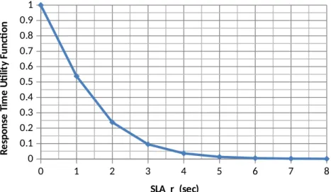
As it can be seen, the response time cost decreases exponentially as the SLA for response time increases. The throughput cost increases linearly with the throughput SLA and the availability cost increases exponentially as the availability SLA goes from 0.9 to 1.0.

Used the following utility function:

U=ω_r2 .0e

−SLA_r

1+e−SLAr +ωx(1−e

−0 .1SLA_x

)+ω_a(10SLA_a−9)

. (4)

The first term in Eq. (3) is the response time utility function, the second term is the throughput utility function, and the third is the availability utility function. Because each of these individual utility functions have their values in the [0,1] range

A cloud user is now faced with the problem of selecting the optimal values of the SLAs that maximize the utility function subject to SLA and cost constraints. This can be cast as the (generally) non-linear constraint optimization problem shown below.

Maximize U=f

(

)

Subject to γ_rmin≤SLA_r≤γ_rmax ₍₆₎

γ_xmin≤SLA_r≤γ_xmax ₍₇₎

γ_amin≤SLA_r≤γ_amax ₍₈₎

Cr

(

)

(

)

(

)

The optimization problem above indicates that values of the SLAs for response time, throughput, and availability have to be obtained so that the utility function is maximized. The SLAs have constraints (minimum and maximum values), which may be inherent to what the cloud provider can offer. There is also a maximum cost constraint

C_{max .}

Provide here a numeric solution for this problem with the following set of parameters

0 1 2 3 4 5 6 7 8 0 0.1 0.2 0.3 0.4 0.5 0.6 0.7 0.8 0.9 1

SLA_r (sec)

R e sp o n se T im e U ti lit y Fu n cti o n

Figure 1 – Response Time Utility Function

0 5 10 15 20 25 30 35 40 45 50 0 0.1 0.2 0.3 0.4 0.5 0.6 0.7 0.8 0.9 1

SLA_x (sec)

Th ro u gh p u t U ti lit y Fu n cti o n

Figure 2 – Throughput Utility Function

0.9 0.91 0.92 0.93 0.94 0.95 0.96 0.97 0.98 0.99 1 0 0.1 0.2 0.3 0.4 0.5 0.6 0.7 0.8 0.9 1

SLA_a (sec)

A va ila b ili ty U ti lit y Fu n cti o n

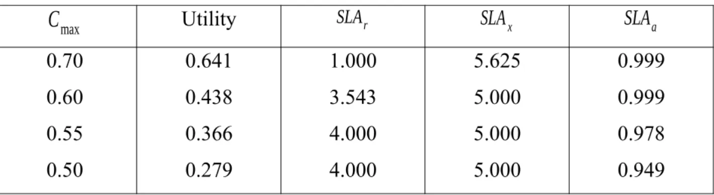
Table 1 shows the results of solving the non-linear constrained optimization

problem for various values of the maximum cost

C

w

,w

,w

decreases from row 4 to row 1. When the user is willing to spend 0.70 cents per transaction, the response time SLA is the best possible (i.e., 1 second), the throughput SLA is slightly above the worst possible value of 5 tps, and the availability is the best possible (i.e., 0.999). As the user is less willing to spend more money per transaction,

the SLAs to be negotiated with the cloud change. For example, for

C

cents, the user will need to settle for a response time SLA of 3.543 sec. The throughput

SLA goes down to its worst value (i.e., 5.0 tps). As the

C

need to be negotiated as shown by the table. As seen in the table, the cloud utility value

decreases as

C

Many optimization solvers can be used to solve the type of non-linear optimization problem discussed above. The NEOS Server for Optimization provides many such options. MS Excel’s Solver (under the Tools menu) can also be used to solve medium scale optimization problems.

Table 1 – Numeric results for optimal SLA selection. Cost is in cents, SLAr _{in sec and}

SLA

C

0.70 0.60 0.55 0.50

0.641 0.438 0.366 0.279

1.000 3.543 4.000 4.000

5.625 5.000 5.000 5.000

0.999 0.999 0.978 0.949

1. Calculate utility functions:

U_r=2. 0e

−SLA_r

1+e−SLAr

, for SLA_r=0,1,…,9;

;

U_x=(1−e−0 .1SLAx), for SLA_x=5,10,…,50; _;

U_a=10SLA_a−9, for SLA_a=0.91,0.92,…,1.

.

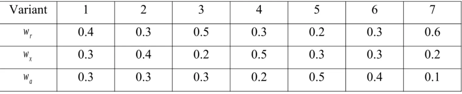
2. Calculate values of global utility according to the variant (Table 2) and equation (4).

Table 2 – Weights associated with response time, throughput, and availability

Variant 1 2 3 4 5 6 7

w_r 0.4 0.3 0.5 0.3 0.2 0.3 0.6

w_x 0.3 0.4 0.2 0.5 0.3 0.3 0.2

w_a 0.3 0.3 0.3 0.2 0.5 0.4 0.1

4. Fill the table:

U_r

U_x

U_a

U