Blind Separation of Nonlinear Mixing Signals Using
Kernel with Slow Feature Analysis
Usama S. Mohmmed
*1, Hany Saber
*21
Department of Electrical Engineering, Assiut University, Assiut 71516, Egypt 2
Department, of Electrical Engineering, South Valley University, Aswan, Egypt 1
Corresponding author [email protected]
Abstract-- This paper describes a hybrid blind source separation approach (HBS S A) for nonlinear mixing model (NL-BS S ). The proposed hybrid scheme combines simply the kernel-feature spaces separation technique (KTDS EP) and the principle of the slow feature analysis (S FA). The nonlinear mixed data is mapped to high dimensional feature space using kernel -based method. Then, the linear blind source separation (BS S ) based on the slow feature analysis (S FA) is used to extract the most slowness vectors among the independent data vectors. The proposed scheme is based on the following four key features: 1) estimating an orthonormal bases, 2) mapping the data into the subspace using this orthonormal bases, 3) applying linear BS S on the mapping data to make the data vectors in the feature spaces are independent, 4) Applying the principle of slow feature analysis on the mapping data to select the desired signals. The S FA provides the dimension reduction according to the most independent and slowing variable signals. Moreover, the orthonormal bases estimation in the wavelet domain is introduced in this work to reduce the complexity of the KTDS EP algorithm. The motivation of using the wavelet transform, in estimating the orthonormal bases, is based on the fact that the low frequency band in the wavelet domain contains the significant power of the signal. The advantages of the proposed method are the fast estimation of the orthonormal bases and the dimension reduction of the estimating data vectors. Performed computer simulations have shown the effectiveness of the idea, even in presence of strong nonlinearities and synthetic mixture of real world data. Our extensive experiments have confirmed that the proposed procedure provides promising results.
Index Term-- Nonlinear blind source separation, slow feature analysis, independent slow feature analysis, slow feature analysis, kernel base algorithm, and kernel trick
I. INT RODUCT ION
The problem of blind source separation (BSS) consists on the recovery of independent sources from their mixture. This is important in several applications like speech enhancement, telecommunication, biomedical signal processing, etc. Most of the work on BSS mainly addresses the cases of instantaneous linear mixture [1]-[5]. Let A is a real or complex rectangular (n×m; n≥m) matrix, the data model for linear mixture can be expressed as follows:
AS(t)
X(t)
(1)Where S(t) rep resents the statis tically independent sources array wh ile X(t) is the array containing the observed signals. For real world situation, however, the basic linear mixing model in equation (1) is too simple for describ ing the observed data. In many applications such as the no nlinear characteristic introduced by preamplifiers of receiving sensors, we can consider a nonlinear mixing. Therefore, a nonlinear mixing is more realistic and accurate than linear model. For instantaneous mixtures, a general nonlinear data model can have the form:
(S(t))
X(t)
f
(2)Where f is an unknown vector of real functions. The linear instantaneous mixing (BSS) can be solved by using independent component analysis (ICA) [4]. The goal of the ICA is to separate the signals by finding indepen dent component from the data signal. It is important to note that if
x and y are two independent random variables, any of their functions f(x) and f(y) are also independent. An even more serious problem is that in the nonlinear case, x and y can be mixed and still be statistically independent. Several authors [6-10] have addressed the important issues on the existence and uniqueness of solutions for the nonlinear ICA and BSS problems. In general, the ICA is not a strong enough constraint for ensuring separation in the nonlinear mixing case. There are several known methods that try to solve this nonlinear BSS problem. They can roughly be divided into algorithms with a parametric approach and algorithms with nonlinear expansion approach. With the parametric mo del the nonlinearity of the mixture is estimated by parameterized nonlinearities. In [8] and [11], neural network is used to solve this problem. In the nonlinear expansion approach the observed mixture is mapped into a high dimensional feature space and afterwards a linear method is applied to the expanded data. A common technique to turn a nonlinear problem into a linear one is introduced in [12].
I.1 Nonlinear mixture model
A generic nonlinear mixture model for blind source separation can be described as follows:
X(t)
A
f
(S(t))
(3) Where S(t) represents the statistically independent sources array while X(t) is the array containing the observed signals and f is unknown multiple-input and multiple-output (MIMO) mapping which called the nonlinear mixing transform (NMT). In order for the mapping to be invertible, we assume that the nonlinear mapping is monotone. We make the assumption here, for simplicity and convenience, that the dimensions of Xand S is equal.
An important special case of the nonlinear mixture is the so-called post-nonlinear (PNL) mixture
(AS(t))
X(t)
f
(4)
Where f is an invertible nonlinear function that operates componentwise and A is a linear mixing matrix, more detailed
n
1,...,
i
,
(t)
S
a
f
(t)
X
m
1 j
j ij i
i
(5)
Applications are found, for example, in the fields of telecommunications, where power efficient wireless communication devices with nonlinear class C amplifiers are used [19] or in the field of biomedical data recording, where sensors can have nonlinear characteristics [20].
In this work, a new method to solve the PNL-BSS problem or the general nonlinear BSS is proposed. In the first step, the nonlinear mixed data is mapped to higher dimensional feature space fk and linear blind source separation algorithm is applied on the mapped data. In the second step, the principle of slow feature analysis is used on the linearly separated data to find the most slow and independent vectors in this feature space. In the following Sections, the kernel-feature Spaces separation technique (KTDSEP) and the principle of slow feature analysis (SFA) will be discussed.
II. KERNEL FEAT URE SPACES AND NONLINEAR BLIND SOURCE SEPARAT ION
In kernel-based learning, the data is mapped to a kernel feature space of a dimension that corresponds to the numb er of training data points. Suppose that the data is Xi (i=1,………..,N), so the idea is to mapping the data Xi into some kernel feature space ƒk by some mapping Φ : Rn→ ƒk. Performing a simple linear algorithm in ƒk, corresponds to a nonlinear algorithm in the input space will solve the separation problem. Essential ingredients to kernel based learning are: (1) support vector machine (SVM) [21] [22] theory that can provide a relation between the complexity of the function class in use and the generalization error, and (2) the famous kernel trick
Φ(y)
Φ(x)
y)
K(x,
(6)Which efficiently computes the scalar product. This trick is essential if ƒk is an infinite dimensional space. Even though ƒk might be infinite dimensional the subspace, where the data lies is maximally N-dimensional. However, the data typically forms an even smaller subspace in ƒk [23]. To map the
nonlinear mixing data X1… XN
n
R
into the feature spaceƒk the kernel trick in Equation (6) must be used, but the high domination mapping data will be. In [21] the idea of estimating the orthonormal bases for subspace ƒk is proposed and these bases is used to map the nonlinear mixed data to the feature space ƒk
For some further points v1,……..,vd
n
R
from the same space, that will later generate a bases in ƒk. The mapping method will be as follows:Consider the mapping points asx
(x1) .. .. (xN)
, andv
(v1) .. .. (vd)
.Assume that the columns of Φv constitute a base of the column space of Φx, so
)
(
and
)
(
)
(
span
rank
d
span
v
x
Tv
v
(7)Moreover, Φv being bases implies that the matrix ΦvT Φv has full rank and its inverse exists. Now an orthonormal bases can be defined as follows:
v v v
2 1
)
(
(8)The column space of which is identical to the column space of Φv. Consequently, the bases
enable us to parameterize allvectors that lie in the column space of Φx by some vectors
in
R
d. The space that is spanned by
is called parameter space. The orthonormal bases Equation (7) enables theworking in
R
d the span of
, which is extremely valuable since d depends solely on the kernel function and the dimensionality of the input space. Therefore, d is independent of N.To map the mixed data from input space to feature space fk the kernel trick is used to perform the following:
d
j
i
v
v
k
v
v
i j i jij v v
...
1
,
with
)
,
(
)
(
)
(
)
(
N
j
d
i
x
v
k
x
v
i j i jij x v
...
1
,
...
1
,
with
)
,
(
)
(
)
(
)
(
(9)
Finally the mapping matrix will be
x v v v x
x
21 )
(
(10)
Which is also a real valued d x N matrix and the matrix
2 1
)
(
v
v is symmetric. Two main problems facing the kernel based algorithm (KTDSEP):
Selecting the points v1,…..,vd to constructed the orthonormal bases
The number of output signals from KTDSEP algorithm will be d signals and we need only n signals where n is smaller than d.
In the traditional KTDSEP algorithms, the random sampling method and the k-mean clustering method are used to find the orthonormal bases. These two techniques increase the complexity of the algorithm. Moreover, the KTDSEP method cannot automatically find n signals out of d signals. The proposed solution by the KTDSEP method [24] is based on the correlation among the original signals and the output signals. In the blind source separation field the original signals is not available, so this technique is not practical. Another proposed solution [21] is done by applying the KTDSEP on the signals two times. This solution will increase the computational complexity of the algorithm.
In this work, after mapping the data, the linear blind source separation algorithm is used. The temporal decorrelation BSS (TDSEP) [24] is used as linear blind source separation algorithm. In the next Sections, the details of our proposed solution will be discussed.
III. SLOW FEAT URE ANALYSIS AND NONLINEAR BLIND SOURCE SEPARAT ION
Slow Feature Analysis (SFA) is a method that extracts slowly varying signals from a given observed signals [25], [26]. Consider an input signal x(t)=[x1(t), . . . ,xN(t)]T, the objective of SFA is to find a nonlinear input-output function g(x) =
[g1(x), . . . , gL(x)]T such that the components of u(t)= g(x(t)) are varying as slowly as possible. The variance of the first derivative is used as a measurement of the slowness. The optimization problem will be as follows:
)
(
))
(
(
2'
t
U
t
U
i
i
(11)Successively for each Ui(t) under the following constraints:
0
)
(
t
u
i(a)
u
i(
t
)
2
1
(b)
0
)
(
)
(
t
u
t
j
i
u
i j
(c)
Where <•>denotes averaging over time. Constraints (a), (b) and (c) ensure that the solution will not be the trivial solution (Ui(t)= const). Constraint (c) provides uncorrelated output signal components and thus guarantees that different components carry different information.
Note that slowly varying signal components are easier to predict and should therefore have strong correlations in time. In the proposed work, the principle of slow feature analysis is used to overcome the main drawback of the kernel base algorithm (KTDSEP) to pickup n signals out of d signals. The slow feature analysis algorithm is motivated by the fact that the linear signals are the slowest varying signals among all the signals [12]. Therefore, the slow feature analysis can be used to pickup n slow varying signals (linear) from d signals. The slow feature analysis algorithm can be summarized in the following steps:
i. Nonlinear expanding the input data.
ii.The nonlinear expanding signal is whitened using eigenvalue decomposition of the zero time-log correlation matrixes.
iii. Derivative the whitened signal is calculated according to
)
(
)
1
(
)
(
y
'
t
y
t
y
t
iv. The rotating matrix Q is calculated using the joint approximate diagonalization (JAD).
v. The eigenvalue and the eigenvectors of Q are evaluated. vi. The dimensional reduction of the signals by is achieved
using the normalized eigenvectors that corresponding to the smallest eigenvalue of the rotation matrix Q.
IV. THE PROPOSED HYBRID BLIND SOURCE SEPARAT ION APPROACH (HBSSA)
One of the most popular methods to solve the problem of the nonlinear mixing model (NL-BSS) is the mapping of the nonlinear mixing data into high dimensional feature space fk.
Then the problem can be handled as a linear problem under some constraints [12], [21]. As mentioned in Section II, the kernel base algorithm (KTDSEP) is depended on mapping the nonlinear mixed data into high dimensional space.
The proposed separation method combines simply the kernel-feature Spaces separation technique (KTDSEP) and the principle of the slow feature analysis (SFA). The estimation of the orthonormal bases is done in the wavelet domain to reduce the complexity of the KTDSEP algorithm. The motivation of using the wavelet transform, in estimating the orthonormal bases, is based on the fact that the low frequency band in the wavelet domain contains the significant power of the signal. Moreover, the SFA is used to select the desired signals from the output signals of the KTDSEP algorithm. The SFA algorithm is motivated by the fact that the linear signals are
the slowest varying signals among all the signals. The orthonormal bases is started by selecting the data vector
v1,………….., vd and testing these vector using Equation (6). This vector is selected using the k-mean clustering in KTDSEP. The wavelet transform is applied on the nonlinear mixed data n-times to select the v1,………….., vd from lowest frequency band. Then, equation (7) is used to find the
orthonormal bases
. The proposed method can be summarized as the follows:1. The wavelet transformed (using wavelet packet) is applied on the nonlinear mixed data n times.
2. The points v1,….., vd are selected fro m the lo west frequency band in the wavelet domain.
3. Equation (7) is used to construct the orthonormal
bases
.4. The kernel t ric k is used to map the mixed data into the nonlinear feature space fk and find d x N matrix
5. The output data ψx are pre-whitened
6. Evaluate n time shifted covariance matrices among the vectors of pre-whitened ψx
7. The joint approximate diagonilaizat ion criteria is used with the n time shifted covariance matrices to estimate the
d x d separating matrix B.
8. The Slow Feature Analysis is applied on the d x d
separation matrix B to get n x d rotation matrix (QASF) as following:
Derivative the whitened signals ψx step (5)
The rotating matrix Q is calculated using the joint approximate diagonalization (JAD).
The eigenvalue and the eigenvectors of Q are evaluated
Applying the dimensional reduction to find n out of d signals by using the n norma lized e igenvectors that corresponding to the smallest n e igenvalue of the rotation matrix Q and find QASF= Q(mxd) x B(dxd) 9. Multiply the QASF by the output d x N, fro m step (5), to
get n x d output signals.
Steps 5, 6 and 7 a re re fer to the TDSEP algorith m and step 8 is the principle of SFA algorithm
V. ASSUMP TIONSAND DEFINITIONS
In the proposed algorith m, there are some assumptions are considered as follows: (1) the source signals must be independent, (2) the number of mixed signals are greater than or equal to the number of the source signals, (3) there are at most one source signal have Gaussian distribution, (4) the nonlinear function f is invertible function, and (5) the mixed matrix must be of full rank.
VI. SIMULAT ION RESULT S AND IMPLEMENT AT ION
Several types of signals are used to evaluate the performance of the proposed technique. To put the results in a comparison form, the same examples in [21] and we introduced a new example.
Experiment 1: In the first experiment, two sinusoidal signals
with different frequencies are used:
T 2 1
(t)
S
(T)]
[S
S(t)
where
S
1(
t
)
sin(
100
t
)
andS
2(
t
)
sin(
42
t
)
,)
(
21
x v v v x
x
with
t
1
,...,
2000
. These source signals are nonlinearly mixed according to the following equation:) ( )
( 2
) ( )
( 1
2 1
2 1
)
(
)
(
t s t
s
t s t
s
e
e
t
X
e
e
t
X
(12)
Here, a polynomial kernel of degree 5 is used,
5
)
1
(
)
,
(
a
b
a
b
k
T (13)In this experiment, 21 points (v1,….,v21) are selected. So we have
ψ
x with size of 21 x 2000. When TDSEP is applied onψ
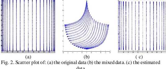
x, 21 different data vectors are generated and the slowfeature analysis generates 2 x 2000 data vectors. Fig. 1 shows the original, the mixing and the estimating sources. Moreover, the scattering plot of the three signals is shown in Fig 2.
Experiment 2: In this experiment, two speech signals, T
2 1
(t)
S
(T)]
[S
S(t)
, of 2000 samples are mixed. Thenonlinear mixing is done using Equation (14). Fig. 3 shows the original, the mixing and the estimating sources. The scattering plot of the original signals, the mixed signals and the estimating signals are shown in Fig 4.
))
(
sin(
)
1
)
(
(
5
.
1
)
(
))
(
cos(
)
1
)
(
(
)
(
1 2
2
1 2
1
t
S
t
S
t
X
t
S
t
S
t
X
(14)
Gaussian radial base function (RBF) Equation (15) is employed with σ = 0.5.
e
σ
b
a
k(a ,b )
2
2
(15)In this experiment, 17 points (v1,….,v17) is selected so the
ψ
xhas a size of 17 x 2000 is estimated. When TDSEP is applied on
ψ
x we will have 17 different data vectors. The slow featureanalysis is used to get 2 x 2000 data vectors from 17 x 2000 different data vectors.
Fig. 1. the original data are the first two signals on the top, the mixing data are in the middle and the recovering data are in the last two rows
(a) (b) ( c)
Fig. 2. Scatter plot of: (a) the original data (b) the mixed data. (c) the estimated data
Experiment 3: In this experiment, the same speech signals in experiment 2 are used. The nonlinear twisted function [12], Equation (16), is used. Fig. 5 shows the original, the mixing and the estimating sources. The scattering plot of the original signals, the mixed signals and the estimating signals are shown in Fig 6.
))
(
5
.
1
sin(
)
6
)
(
3
)
(
(
)
(
))
(
5
.
1
cos(
)
6
)
(
3
)
(
(
)
(
1 1
2 2
1 1
2 1
t
S
t
S
t
S
t
X
t
S
t
S
t
S
t
X
(16)
The same RBF in Equation (15) with σ = 0.5 is employed in this experiment. 20 points (v1,….,v20) is selected so we will get
ψ
x of size 20 x 2000. When TDSEP is applied onψ
x we willhave 20 different data vectors. The slow feature analysis is used to get 2 x 2000 data vectors from 20x2000 different data vectors.
Fig. 3. the original data are the first two signals on the top, the mixing data are in the middle and the recovering data are in the last two rows
(a) (b) ( c)
Fig. 5. the original data are the first two signals on the top, the mixing data are in the middle and the recovering data are in the last two rows
(a) (b) ( c) Fig. 6. (a) scatter plot of the original data. (b) Scatter plot of the mixed data.
(c) scatter plot of the estimated data
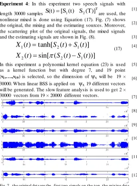
Experiment 4: In this experiment two speech signals with
length 30000 samples
T 2 1
(t)
S
(T)]
[S
S(t)
are used, thenonlinear mixed is done using Equation (17). Fig. (7) shows the original, the mixing and the estimating sources. Moreover, the scattering plot of the original signals, the mixed signals and the estimating signals are shown in Fig. (8).
))]
(
)
(
(
sin[
)
(
)]
(
)
(
tanh[
)
(
1 2
2
1 2
1
t
S
t
S
t
X
t
S
t
S
t
X
(17)In this experiment a polynomial kernel equation (23) is used as a kernel function but with degree 7, and 19 point (v1,….,v19) is selected, so the dimension of
ψ
x will be 19 ×30000. When linear BSS is applied on
ψ
x 19 different vectorswill be generated. The slow feature analysis is used to get 2 × 30000 vectors from 19 × 20000 different vectors.
Fig. 7. the original data are the first two signals on the top, the mixing data are in the middle and the recovering data are in the last two rows
(a) (b) ( c)
Fig. 8. (a) scatter plot of the original data. (b) Scatter plot of the mixed data. (c) scatter plot of the estimated data
VII. CONCLUDING REMARKS
In this paper, a novel hybrid scheme to solve the problem of blind source separation in nonlinear mixing model (NL-BSS) is proposed. The proposed hybrid scheme combines simply the kernel-feature Spaces separation technique (KTDSEP) and the principle of the slow feature analysis (SFA). The proposed algorithm overcomes the drawback of the kernel base nonlinear blind source separation algorithm (KTDSEP). The slow feature analysis principle is used in selecting the n
separated signals from d output signals. Moreover, new approach to construct the orthonormal bases by selecting the bases points from the lowest frequency band in the wavelet transformed is introduced. The advantage in performance of HBSSA lays in the complexity reduction in the orthonormal bases estimation process and the fast selection of the desired signals from the output signals of the KTDSEP algorithm.
REFERENCES
[1] Amari, A. Cichocki, and H. H. Yang. "A new learning algorithm for blind signal separation." In NIPS 95, pp. 882 –893. MIT Press, 1996.
[2] Bell and T . Sejnowski. ―Information-maximization approach to blind separation and blind deconvolution" Neural Computation, vol. 7, pp.1129–1159, 1995.
[3] Cardoso. "infomax and maximum likelihood for source separation" IEEE Letters on Signal Processing, vol. 4, pp.112 –114, 1997. [4] W. Lee, M. Girolami, and T . Sejnowski. "Independent component analysis using an extended infomax algorithm for mixed sub-Gaussian and super-sub-Gaussian sources." Neural Computation, vol. 11, pp.417–441, 1999.
[5] D.-T . Pham, and J.-F. Cardoso, ― Blind separation of instantaneous mixtures of non-stationary sources‖, IEEE T rans. on Signal Processing, vol. 49, no.9, pp. 1837 -1848, Sep. 2001.
[6] C. Jutten and A. T aleb, ―Source separation: from dusk till dawn,‖ in Proc. 2nd Int. Workshop on Independent Component Analysis and Blind Source Separation (ICA2000), pp. 15–26, Helsinki, Finland, 2000.
[7] A. Hyv¨arinen and P. Pajunen, ―Nonlinear independent component analysis: Existence and uniqueness results,‖ Neural Networks, vol. 12, no. 3, pp. 429–439, 1999.
[8] A. T aleb and C. Jutten, ―Source separation in post -nonlinear mixtures,‖ IEEE Trans. on Signal Processing, vol. 47, no. 10, pp. 2807–2820, 1999.
[9] A. T aleb, ―A generic framework for blind source separation in structured nonlinear models,‖ IEEE T rans. on Signal Processing, vol. 50, no. 8, pp. 1819–1830, 2002.
[10] J. Eriksson and V. Koivunen, ― Blind identifiability of class of nonlinear instantaneous ICA models,‖ in Proc. of the XI European Signal Proc. Conf. (EUSIPCO 2002), vol. 2, T oulouse, France, , pp. 7–10, September 2002.
[11] Luis B. Almeida, "Linear and nonlinear ICA based on mutual information‖ the MISEP method, Signal Processing, Special Issue on Independent Component Analysis and Beyond 2004, vol. 84, no.2, pp.231–245.
[13] T aleb and C. Jutten. Nonlinear source separation: T he post -nonlinear mixtures. In Proc. European Symposium on Artificial Neural Networks, pp. 279–284, Belgium, 1997.
[14] T .-W. Lee, B.U. Koehler, and R. Orglmeister. Blind source separation of nonlinear mixing models. IEEE International Workshop on Neural Networks for Signal Processing, pp. 406–415, 1997.
[15] H.-H. Yang, S. Amari, and A. Cichocki. Information -theoretic approach to blind separation of sources in non -linear mixture. Signal Processing, vol. 64, no.3, pp.291 –300, 1998.
[16] A. T aleb and C. Jutten. Source separation in post -nonlinear mixtures. IEEE T rans. on Signal Processing, vol. 47, no.10, pp.2807–2820, 1999.
[17] A. Ziehe, M. Kawanabe, S. Harmeling, and K.-R. M¨uller. Separation of post -nonlinear mixtures using ACE and temporal decorrelation. In T .-W. Lee, editor, Proc. Int . Workshop on Independent Component Analysis and Blind Signal Separation (ICA2001), pp. 433–438, San Diego, California, 2001. [18] C. Jutten and J. Karhunen. Advances in nonlinear blind source
separation. In Proc. of the 4th Int. Symp. on Independent Component Analysis and Blind Signal Separation (ICA2003), pp. 245–256, Nara, Japan, Invited paper in the special session on nonlinear ICA and BSS, April 2003.
[19] L. E. Larson. "Radio frequency integrated circuit technology low-power wireless communications". IEEE Personal Communications, vol. 5, no. 3, pp.11–19, 1998.
[20] A. Ziehe, K.-R. M¨uller, G. Nolte, B.-M. Mackert, and G. Curio. Artifact reduction in magnetoneurography based on time-delayed second-order correlations. IEEE Trans. Biomed. Eng., vol. 47 , no. 1, pp. 75–87, 2000.
[21] Harmeling, S., Ziehe, A., Kawanabe, M., and Müller, K. -R. "Kernel-based nonlinear blind source separation." Neural Computation, vol. 15, pp: 1089–1124, 2003.
[22] N. Cristianini and J. Shawe-T aylor.(200) " An Introduction t o Support Vector Machines." Cambridge University Press, Cambridge, UK, 2000
[23] B. Schölkopf, S. Mika, C.J.C. Burges, P. Knirsch, K.-R. Müller, G. Rätsch, and A.J. Smola." Input space vs. feature space in kernel-based methods." IEEE Transactions on Neural Networks, vol. 10, no. 5 pp.1000–1017, 1999
[24] A. Ziehe and K.-R. Müller. "T DSEP —an efficient algorithm for blind separation using time Structure,‖ In Proc. Int. Conf. on Artificial Neural Networks (ICANN’98), pp. 675–680, 1998 [25] Laurenz Wiskott "Slow feature analysis: a theoretical analysis of
optimal free responses" Neural Computation, vol. 15, pp.2147 - 2177, 2003