Functional Modelling of Microarray Time Series

FUNCTIONAL MODELLING OF MICROARRAY TIME SERIES

WITH COVARIATE CURVES

Maurice Berk

Department of Mathematics, Imperial College London Giovanni Montana

Department of Mathematics, Imperial College London

1. INTRODUCTION

Biological systems are inherently dynamic and gene expression levels may be tempo-rally regulated for a wide range of reasons including the cell cycle, circadian rythms, developmental processes or in response to stimuli (e.g. drug treatment or environmen-tal stress) (Spellmanet al., 1998; Wang and Kim, 2003; Calvanoet al., 2005). Microarrays are a high throughput assaying technique for measuring these expression levels of thou-sands of genes simultaneously. Each microarray hybridisation provides a snapshot of expression levels at a single point in time; by carrying out sequential hybridisations on biological samples arising from the same source (e.g. a human patient), the evolution of these expression levels over time can then be elucidated.

The resulting microarray time series give rise to data that possess certain character-istics which make their analysis particularly challenging. Specifically, due to the large number of genes under study simultaneously, the data is very highly dimensional and there are many more genes than there are time points. Each time series will be repli-cated typically no more than ten times, and experiments with no replication are not uncommon. The number of genes will often number in the tens of thousands while there are rarely more than ten time points. Even with the falling cost of microarray technology, the limiting factor is often the ability to obtain biological samples which may be restricted due to ethical concerns or other practical, experimental issues. Other challenges include the fact that the data is noisy, with frequent missing observations, and individual heterogeneity.

female and ten male adult human subjects over a period of 6 months, in order to charac-terise the change in gene expression levels over time in healthy humans. Figure 1 shows some of the raw data for a probe corresponding to the TMEFF1 gene from this exam-ple data set where some of the characteristics discussed above can be seen to manifest themselves. A key aspect of human data sets is that the gene expression levels are often collected with covariates - for example, the individual’s age, sex and other phenotypic data such as height or weight may be recorded. In the case study, the individuals were stratified by age and gender which allows us to explore not only the evolution of gene expression levels over time but also which genes are differentially expressed between the two gender or age groups.

When modelling experimental data arising from longitudinal microarray experi-ments there are three distinct challenges: (a) modelling each individual time series, across all genes and individuals, (b) accounting for the correlation between individu-als on a gene by gene basis and (c) modelling the correlation between genes. Account-ing for each of these sources of correlation — the temporal, the within-gene (between-individual) and the between-gene — is vital for obtaining better parameter estimates and avoiding a loss of power when testing for genes which are differentially or temporally expressed. With less than 10 timepoints, achieving (a) is not possible with standard time series analysis techniques — it is unlikely, for instance, that we would observe any pe-riodicity. Instead, a field which has proven to be quite successful in this area is that of functional data analysis (FDA). In the FDA paradigm, it is assumed that our observa-tions are noisy realisaobserva-tions of an underlying smooth function of time which is to be estimated. These estimated functions, or curves, are then treated as the fundamental unit of data in any subsequent analysis. Formally, the signal-in-noise model assumed is that observationy_itaken at timet_i is given by

y_i= f(t_i) +εi (1)

where f(·)is the function of interest to be estimated andε_i is an error term. Typically the infinite dimensional function f(·)is projected onto some finite dimensional basis using parameterisations such as splines, wavelets or fourier bases. In our discussion we will focus on splines in particular as these regularly occur in the literature in terms of both microarray and functional data analysis. For a thorough treatment of FDA, the monograph Ramsay and Silverman (2005) provides an excellent introduction.

In a longitudinal study, for a particular gene, observations will be collected on not just a single functionf(·), but a collection ofnfunctionsf_i(·),i=1,· · ·,n, one for each individual biological unit. Often the main quantity of interest is the population mean functionµ(·)characterising the overall population gene expression level over time. In this case we extend the signal-in-noise model (1) so that the jth observation on individ-ual at timet_{i j} is given by

y_{i j}=µ(t_{i j}) +f_i(t_{i j}) +εi j (2)

both considered functions. Functionµ(·)is treated as a fixed-effect as it is assumed to be some fixed, but unknown, population function to be estimated. In constrast, the functions f_i(·),i=1,· · ·,nrepresent a random sample from the population as a whole and are assumed to be i.i.d realisations of an underlying stochastic process. Model (2) has appeared in a number of different forms depending upon the exact parameterisa-tion of the fixed- and random-effects. For instance, Guo (2002) models both as cubic smoothing splines while Rice and Wu (2001) prefer a B-spline representation.

The task of handling correlations amongst the genes has, to date, generally been overlooked by researchers. It is a challenging, open problem to model both the between-and within-gene correlation simultaneously given the size of the data. Although it is well known that genes are co-regulated, for the sake of tractability the most common approach is to simply model each gene independently. In other words, given the frame-work outlined thus far, each gene would be modelled as a separate functional mixed-effects model.

In this paper we propose a functional-mixed effects model and a framework for estimation and testing in one-sample problems. The model enables the estimation of a mean response curve with the inclusion of covariates, such as gender and age, also modeled as time-varying smooth functions. We also show how a functional PCA can be applied to the estimated mean curves in order to identify the principal modes of functional variation in the data set, and visually represent the entire set of genes in a low-dimensional plot.

The structure of the paper is as follow. Section 2 provides a description of a data set, previously collected and analysed by Karlovichet al.(2009), that we use here as a case study. The proposed model, inferential procedures and functional PCA are provided in Section 3. In Section 4 we present the experimenal results obtained in the context of our case study. In Section 5 we discuss how our methodology compares to related models that have appeared in the literature and compare our experimental results to that of the original study, as well as highlight some of the biological implications. Finally, we conclude in Section 6.

2. DATA DESCRIPTION

The data set used in our case study is taken from Karlovichet al.(2009). The purpose of the study was to characterise the gene expression levels of healthy human individuals over a period of 6 months. 22 subjects were studied, with gene expression levels assayed from blood samples at days 1, 14, 28, 90 and 180. One subject developed lung cancer during the course of the study and died prior to Day 180, thus contributing only a partial time series. All other individuals completed the study and were observed at all 5 time points. Twelve of the individuals were female and ten were male. In the original study, the subjects were divided into two age groups, with the younger group taken to be those subjects less than or equal to 55 years of age, and the older group those subjects over 55.

modelled as

y_{i t}=µ+αi+βgg e nd e ri+βaa g ei+βtt i met+εi t

This is a standard linear mixed-effects model. µ is the average gene expression level across all individuals after controlling for gender, age and time effects.αiis an individual

specific term allowing for a deviation in terms of the intercept of the model. Theβg,

βaandβt parameters separate out the gender, age and time effects respectively while

εi t is an error term.

The model and study design permitted a wide range of biological issue to be ex-plored. Using t-tests, the significance of the age and gender effects was determined. After correcting for multiple-testing by controlling the false discovery rate (FDR) using the procedure of Benjamini and Hochberg (1995), no genes showed a significant age ef-fect. This was somewhat unexpected given previous studies (Eadyet al., 2005; Whitney

et al., 2003; Tanget al., 2004) but it was noted that these age effects might be harder to detect in blood than in other tissuses. 78 unique gender genes were identified including XIST, responsible for deactivating one of the X chromosomes in females in order to ensure dosage equivalence, and 23 genes mapped to the Y chromosome. Temporally regulated genes were identified by performing pairwise comparisons between Day 14 and Day 1, Day 28 and Day 14, and Day 180 to Day 90. This was partly due to con-cerns about a potential batch effect, as Days 1, 14 and 28 were processed in one batch, with Days 90 and 180 being processed in a second batch. No temporally regulated genes were identified in the Day 14 vs Day 1 or the Day 28 vs Day 14 comparisons, but 248 probes were found to be differentially expressed when comparing Day 180 to Day 90, corresponding to 157 unique genes.

Our proposed approach is to replace the original linear mixed-effects model with a functional one. The age and gender effects will be modelled as functions of time, along with the mean and individual curves. To avoid over-parameterisation, all curves will be represented using smoothing splines. The result is a flexible model which permits the interaction of age and gender with time, if the data supports it. During our preprocess-ing we found little evidence of a batch effect and we will use the entire time course to identify temporally regulated genes, on the basis of the fitted mean function.

3. METHODS

We propose the following functional mixed-effects model for the data described in Sec-tion 2. Each gene is modelled independently. For a given gene, the observed gene expression level for individuali at timet_{i j}is given by

y_i(t_{i j}) =µ(t_{i j}) +αk(ti j) +βl(ti j) +γi(ti j) +εi j (3)

whereµ(·)models the mean expression levels across all individuals after accounting for age and gender effects;αk(·)is the gender effect for genderk to which individual i belongs withk ={Male, Female};β

l(·)is the age group effect for group l to which

individuali belongs where l ={Young, Old};γ

individuali andεi j is an error term. The functionsµ(·),αk(·),βl(·)andγi(·)are

as-sumed to be smooth functions of time which we wish to estimate based on the noisy observations. We treatµ(·),α

k(·)andβl(·)as fixed-effects, unknown population

func-tions to be estimated, and theγi(·)functions which are treated as random-effects as they

represent a random sample of functions from the population as a whole. Formally, the γi(·)are assumed to be i.i.d. realisations of an underlying Gaussian Process with mean

0 and covariance functionδ(r,s).

The functions can be parameterized in a number of ways but we favour smooth-ing splines as these offer a fine degree of control over the amount to which the data is smoothed. Writing the vector of all observed time points for individuali asti =

[t_i1,t_i2,· · ·,t

i ni]

T _wheren

i is the total number of observations on individuali, (3) can

be written in matrix form as

yi=Xiµ+Xiαk+Xiβl+Xiγi+εi (4)

whereyi= [yi(ti1),yi(ti2),· · ·y_i(t_{i n} i)]

T _andε

i= [εi1,εi2,· · ·,ε_{i n} i]

T _{are vectors of length}

n_i and µ= [µ(τ₁),µ(τ₂),· · ·,µ(τ_M)]T is a vector of length M. The vectorsα_k, β_l and γ_i are defined similarly to µ. The values τ₁,τ₂,· · ·,τ_M denote the distinct de-sign time points, of which there are M in total, and ti may differ from these may

differ if individual i has missing data or duplicate observations for some time points. The matrixXi is an incidence matrix of dimensionni×M where each row x_{i j} con-tains all zeroes aside from the column m where t_{i j} = τm. Further details on

form-ing the incidence matrices and an example can be found in Appendix A.1. Recall that γi(·)∼GP(0,δ),i =1,· · ·,n, then the vectorsγ_iare multivariate-normally distributed with mean0and covariance matrixD whereD(r,s) =δ(τr,τs). Similarly the noise

termεi is multivariate-normally distributed with mean 0 and covariance matrixRi,

and we assume that the vectorsγi andεi are independent. For simplicty we assume

that Ri =σ2Ini×ni, although a more complicated structure could be modelled at the expense of fitting more parameters. It is further necessary to impose the identifiabil-ity constraint that the age and gender fixed-effects for the two groups sum to zero, i.e.

αma l e+αf e ma l e=0andβyo un g+βo l d=0. For simplicity, therefore, we model a single

gender and age effect, α=αf e ma l e andβ=βo l d respectively. These constraints can

equivalently be expressed be rewriting (4) as

yi=Xiµ+Wiα+Ziβl+Xiγi+εi (5)

where

Wi=

−X_i ifiis male Xi ifiis female Zi

=

−X_i ifiis young Xi ifiis old

Letη= [µ,α,β]T_{, then (5) can be rewritten more compactly as}

yi=X ∗

where

X∗

i =

Xi Wi Zi

Finally, the complete data vector for all individuals,y, can be expressed as

y=X∗

η+Xeγ+ε (6)

wherey= [yT 1,y

T 2 ,· · ·,y

T n]

T _{is anN=}P

ini length vector, andγ andεare similarly

defined,X∗

= [X∗ 1

T_,X∗ 2

T_{,· · ·X}∗ n

T_]T _{is anN×3Mmatrix and}

e

X=d ia g(X1,X2,· · ·,X_n) is anN×nM matrix, with thed ia g(·)operator denoting a block diagonal matrix. The vectorsγ andεare both multivariate-normally distributed with mean0and covariance matrixDe=d ia g(D,· · ·,D)andR=d ia g(R₁,R₂,· · ·,R_n)respectively.

3.1. Parameter Estimation

Model (6) is in the form of the standard linear mixed-effects model (Laird and Ware, 1982). Standard practice for obtaining estimates of the fixed- and random-effects, ηˆ andγˆi,i =1,· · ·,n would be to maximise the joint likelihood ofηandγ_i (Robinson, 1991). This is equivalent to minimising the following generalized log likelihood (GLL) criterion

GLL= (y−X∗η−Xeγ)TR−1(y−X∗η−Xeγ) +log|De| (7)

+γT

e

D−1

γ+log|R|

However, in our model the fixed- and random-effects are the fitted values of the smooth-ing spline estimates of the functionsµ(·),α(·),β(·),γ

i(·),i=1,· · ·,n, and it is necessary

to incorporate a penalty term for the roughness of the smoothing splines into the like-lihood. ThepenalizedGLL is then given by

P GLL=GLL+λγ

n

X

i=1

(

Zb

a

[γ′′ i (t)]

2_{d t}

)

+λ

Zb

a

[µ′′

(t)]2d t (8)

+λ

Zb

a

[α′′

(t)]2d t+λ

Z b

a

[β′′

(t)]2d t

where the integrals quantify the roughness of the curves µ(·), α(·), β(·), γ_i(·),

i=1,· · ·,nin terms of their squared second derivative, although other penalties could be used. The scalarsλandλ_γ are positive-valued smoothing parameters that control the roughness of the fit. For a given smoothing spline fit,λ=0 would correspond to an in-terpolation of the data points while asλtends to infinity, the fit tends to a straight line. Note that the same smoothing parameterλis used for the three fixed-effects functions, µ(·),α(·),β(·), and similarly the same smoothing parameter,λ_γ, is used for all random-effect functionsγi(·),i =1,· · ·,n. This is conceptually justified as each functionγi is

to envisage selecting a separate smoothing parameter for each fixed- and random-effect function, albeit at the expense of a far greater computational cost.

Minimization of (8) requires calculation of the integral of the squared second derivative of the fixed- and random-effects. In the case of cubic smoothing splines, for a given function f(t) observed at time points t₁,t₂,· · ·,t

n such that f =

[f(t₁),f(t₂),· · ·,f(t_n)]T, there is a roughness matrix G which can be calculated in a computationally efficient manner that satisfies:

Zb

a

[f′′

(t)]2d t =fTG f

this result can be found in Green and Silverman (1994) and we have reproduced the derivation in Appendix A.2 for completeness. Incorporating the roughness matrix into (8) gives

P GLL = GLL+λ_γ

n

X

i=1

γT

i Gγi+λ(µTGµ+αTGα+βTGβ)

= GLL+λ_γγT

e

Gγ+ληT

G∗

η

whereGeis a block diagonal matrix comprised of the matrixGrepeatedntimes.

Simi-larly,G∗

is a block diagonal matrix comprised ofGrepeated three times.

After a rearrangement on the terms featuring in the penalised log-likelihood, the model can be re-written in terms of the regularised covariance matrices

e

D_γ= (De−1+λ_γG)e −1 andV = XeDe_γXeT +R, so called because the matrix De_γ is

ob-tained by regularising the covariance matrixDe with the term λ_γGe. This method of

imposing the smoothness constraints by regularisation of the covariance matrix can be credited to Wu and Zhang (2006).

Minimising (8) gives the BLUE and BLUP of the fixed- and random-effects as

ˆ

η= (X∗T_V−1

X∗

+λG∗

)−1

X∗T_V−1

y (9)

ˆ

γ=De_γXeTV−1(y−X∗η) (10)

The discussion thus far has assumed that the variance components D and σ2 _were

known. Of course, in practical applications this will not be the case. Assuming the random-effectsγiand error termsεare known, the maximum likelihood estimatorsDˆ

andσˆ2_{are given as}

ˆ D= 1

n n

X

i=1

γiγ T

i σˆ

2₌ 1 Nε

T

ε (11)

As the random-effectsγi and error terms are not, in fact, directly observed, we resort

to the Expectation-Maximisation algorithm where they can be treated as missing data. In this procedure the sufficient statistics of Dˆ and σˆ2 _{— γ}

respectively — are replaced by their conditional expectations which are calculated at the E-step. In the M-step, the maximum likelihood estimators are then calculated having replaced the sufficient statistics by these conditional expectations, which are given by

E[γiγiT|y,η= ˆη] = γˆiγˆiT + ˆDγ−Dˆ_γXT

i V

−1

i XiDˆγ (12)

E[εT_ε

|y,η= ˆη] = εˆTεˆ+ ˆσ2N−σˆ4t r(V−1) (13)

wheret r(·)denotes the trace of a matrix andV

i=XiDγXiT +σ 2_I

ni×n_i. Derivations of

these conditional expectations are given in Appendix A.3.

3.2. Model Selection

Thus far we have treated the smoothing parametersλandλγ as fixed. In reality,

opti-mal values of these parameters must be found using a model selection procedure. Guo (2002) made use of the relationship between a smoothing spline and a linear mixed-effects model in order to treat the smoothing parameters as variances components that could be estimated during the normal course of the EM-algorithm. We prefer, however, to dissociate the model selection from parameter estimation and numerically optimise over the two dimensional space of non-negative reals (Λ×Λ_γ) as this is a much more flexible approach. There are a number of different criteria for scoring the smoothing parameters, all of which essentially trade off between model fit and model complexity.

Maet al.(2006)’s smoothing-spline clustering approach for microarray data, for in-stance, employed Wahba (1977)’s generalized cross validation (GCV) criterion. It is well known, however, that GCV tends to undersmooth (Lee, 2003). Alternatively, we can employ either the Akaike Information Criterion (AIC) or the Bayesian Information Criterion (BIC):

AI C(λ,λ_γ) =−2lik+2df

B I C(λ,λ_γ) =−2lik+l o g(N)df

These two criteria both score the smoothing parameters in terms of the likelihood — measuring the model fit — adjusted for a penalty term for the model complexity, in terms of degrees of freedom. The difference lies in the size of the penalty term, with BIC giving more conservative results whenl o g(N)>2, in other words when there are more than 9 data points.

3.2.1. Smoother Matrices

In order to evaluate the criteria, it is necessary to calculate the degrees of freedom of the model. As per Bujaet al.(1989), the degrees of freedom associated with the fixed-and rfixed-andom-effects,ηandγ, can be expressed as the trace of some smoother matrixA such thatyˆ=Ay. Equivalently, it is useful to determine the two smoother matrices A= Aη+Aγ so that the degrees of freedom of the fixed- and random-effects can be

accounted for separately.

Recall that the fitted values of the fixed-effects at the design time points can be writ-ten asX∗_ˆ

η. Replacingηˆwith (9) gives

X∗_ˆ

η=X∗

(X∗T_V−1

X∗

+λG∗

)−1

X∗T_V−1

y=A_ηy

and so the smoother matrixAηis given by

A_η=X∗

(X∗T_V−1

X∗

+λG∗

)−1

X∗T_V−1

Similarly, the fitted values of the random-effects at the design time points can be written asXeγˆ, which gives

e

Xγˆ=XeDe_γXeTV−1(I_N−A_η)y=A_γy

The degrees of freedom of the model can then be calculated asd f =t r(Aη+Aγ) +1,

which is the trace of the smoother matrix plus an additional paramter for fitting the noise varianceσ2_.

With the scoring function in place any kind of two-dimensional optimisation rou-tine can be used, although in practice a simple grid search or sequential line optimisa-tion is recommended (Wu and Zhang, 2006). We have found that a more sophisticated simplex-search optimiser (Nelder and Mead, 1965) can be employed without incurring a significant computational cost. This allows optimisation over the two smoothing pa-rameters λand λ_γ simultaneously without needing to calculate the derivative of the criterion.

3.3. Confidence Bands

Pointwise confidence bands at the design time points for each of the fixed-effects func-tions can be determined either theoretically or using a bootstrap resampling procedure. In the case of the former, we have

c ov(ˆη) = (X∗T_V−1

X∗

+λG∗

)−1

X∗T_V−1

X∗

(X∗T_V−1

X∗

+λG∗

)−1

asµ(τˆ i)±z

p

c ov( ˆµ(τi)), wherezis the critical value under the normality assumption

such thatφ(z) =1−1

2α. These bands can be calculated for the other fixed-effectsαˆand

ˆ

βin an identical fashion.

Alternatively, confidence intervals can be estimated by resampling the between- and within-individual residuals. To construct a bootstrapped sample for a single individ-ual, first one of the individual functions γi is randomly selected and evaluated at the

design time points - denote this vector asγ∗

. Next,M residuals from the noise vector

ε, are resampled with replacement, writing this vector asε∗

. Then, the bootstrapped observation vectory∗

is given by

y∗₌

µ+α∗₊

β∗₊

γ∗₊

ε∗

whereα∗₌

αif the individual is female and−αotherwise, similarly forβ. This process is then repeated fornindividuals, sampling the individual functions with replacement, to give a complete bootstrapped data set. The model is then fit to this resampled data and new estimates for the fixed-effects obtained. Repeating this process for a large number of iterations gives a large number of fixed-effects estimates from which the confidence bands at a given significance level can be determined empirically.

3.4. Testing for temporal regulation and other effects

Fitting model (6) allows us to separate out the mean, age and gender effects for each gene. It is then possible to determine whether there is a significant group or gender effect by testing the null hypothesis that the corresponding population coefficients are zero. As the effects are modelled as functions, a natural way to quantify their size is theL₂norm. For instance, the hypothesis of absence of an age effect, for a given gene, versus the alternative hypothesis of an age affect, can be framed as

H₀:||α(·)||

2=0, H1:||α(·)||2>0

which is tested using theL2 norm of the estimated coefficients.

Assessing the statistical significance in settings similar to ours is complicated by the fact that the sample sizes are generally very small. On the basis of this, and in agree-ment with previous published studies, we suggest deteriming the null distribution em-pirically by using data resampling schemes. For example, in Storeyet al.(2005), the null distribution of their F-type test-statistic was determined using a nonparametric boot-strap procedure by resampling the individual effects and error terms with replacement. In out study, the null distribution of the L₂ norm of the age and gender effects has been estimated empirically using a permutation procedure where the class assignments — male/female or young/old — are randomly permuted. We take a similar approach when testing for temporal regulation. In this case, the null hypothesis of no change over time is formulated as||µ′(·)||

2=0 whereµ ′

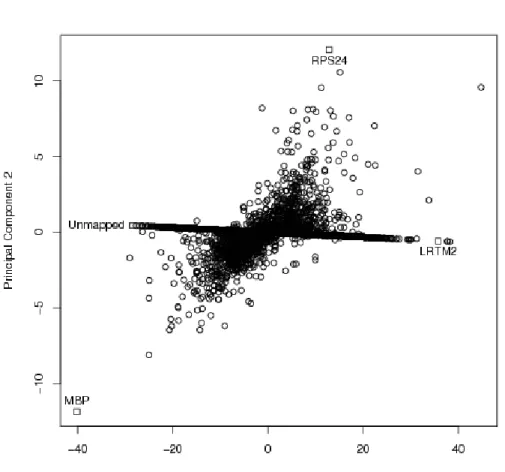
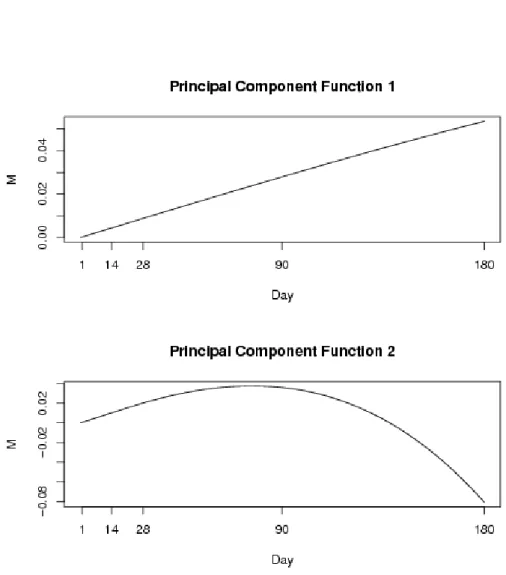
3.5. Functional Principal Components Analysis

Fitting model (6) to each gene yields a set of mean curvesµi(t),i=1,· · ·,GwhereGis

the total number of genes in the data set. Performing a functional PCA (fPCA) (Ramsay and Silverman, 2005) on this set of curves allows us to identify the main patterns of vari-ation across all genes. We perform this analysis in two stages: (1) the data are smoothed by fitting model (6) to each gene (2) a fPCA is then performed on the smoothed data — in the form of the set of curvesµi(t),i=1,· · ·,G. Alternative methods of fPCA such

as Jameset al.(2000), which estimate and smooth the PCs directly, cannot be applied in this case where there are two levels of variation — the between and within-gene. Further details of our approach are given below.

Initially, each curve is discretised on a fine grid ofnequally spaced points across the range of the time course. If there areN curves in total, this yields a data matrixX, of dimensionN×n, and a standard PCA can then be performed onX. As routinely done, this entails solving the eigenequation

Vu=λu (14)

whereV=N−1

XT_{Xis the sample covariance matrix ofX,λis one of the eigenvalues of}

V, anduis one of the eigenvectors, or principal components. In the functional setting, we replaceV by a covariance functionv(s,t), anduby a function ofs,ξ(s)such that the eigenequation (14) becomes

Z

v(s,t)ξ(t)d t=ρξ(s) (15)

for a given value ofs. Noting that after discretisation of the curves the elements of the matrixV=v(s_j,s_k)wherej andkare any of thendiscretised points on the fine grid, the integral in (15) can be approximated as a summation such that

Z

v(s,t)ξ(t)d t=w n

X

k=1

v(s,s_k)ξ˜k

wherewis the spacing between the points on the fine grid, and ˜ξk are the discretised

values of the functionξ(s). The approximate discrete form of the functional eigenequa-tion is therefore

wVξ˜=ρξ˜

which corresponds to (14) with ρ= wλ. Assuming the eigenvectors obtained from the standard PCA have been normalised, the equivalent functional constraint that

R

ξ(s)2_{d s = 1 is achieved by enforicingw||ξ}˜_||2 _{= 1. The function ξ(·)is then}

re-covered by interpolating the points ˜ξ. Assuming the grid is fine enough, the choice of interpolation method is almost irrelevant.

retaining enough PCs to explain most of the variation in the data. AssumingKPCs are retained, for curveiwe have

y_i(t) =µ(t) +

K

X

k

κi kξˆk(t) +εi(t)

whereκi kare the PC loadings for curve i. These can be estimated by minimising the

residualsy_i(t)−PK

kκi kξˆk(t), which in practice again requires discretisation of the curve i, and the PCsξˆk(t).

4. RESULTS

We fit the functional mixed-effects model described in Section 3 to the example data set described in Section 2, independently for each probe. Convergence of the EM al-gorithm was confirmed by convergence of the variance components estimatesσˆ2_and

ˆ

Dand typically took around 30 iterations. 100 iterations of the simplex optimisation procedure were used to select the smoothing parameters. After obtaining estimates of the mean, age and gender effects, and individual curves, these were assessed for signifi-cance. To relieve some of the computational burden, permuted null test statistics were shared across all genes - theoretical results justifying this pooling can be found in Storey

et al. (2004). Each gene was permuted 32 times, yielding in excess of 1 million null test statistics for each comparison. From these null distributions, empirical p-values were calculated, which were then corrected for multiple testing using the procedure of Benjamini and Hochberg (1995) to control the FDR at 10%.

After applying multiple testing corrections, no significant age genes were identified, as in the original analysis. 21 probes were found to be gender specific. Two of these 21 probes can be found on the Y-chromosome but are not mapped to any known genes. The remaining probes correspond to 7 known genes and 2 open reading frames, given in Table 2. Aside from XIST which, as discussed in Section 2 is only expressed in females and is responsible for X-chromose inactivation to facilitate dosage equivalence between the sexes, all significant genes and the two open reading frames are found on the Y-chromosome.

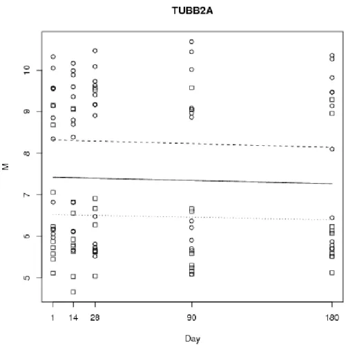
The highest ranked gender-effect gene on an autosomal chromosome was found to be TUBB2A, located on chromosome 6 and ranked number 23, with an associated FDR of 13%, hence of borderline significance. The gene and fitted mean and gender-effect curves is plotted in Figure 3, where a definite difference between the two groups is apparent, corresponding to between a 3- and 4-fold difference in expression levels.

TABLE 1

19 probes found to be significantly differentially expressed according to gender by Karlovich et al.(2009), with a mean log-transformed signal intensity greater than or equal to 7.

Gene Name Chromosome Affymetrix ID Fold Change

- - 211074_at 0.82

EIF1AX X 201019_s_at 0.86

TMEFF2 M 224321_at 0.87

FLOT1 6 210142_x_at 0.87

EIF2S3 X 224936_at 0.90

RPS4X X 213347_x_at 0.91

MGC71993 17 224573_at 0.93

EEF1A1 1 213477_x_at 1.05

EEF1A1 6 206559_x_at 1.07

SPOP 17 204640_s_at 1.07

ERBB2IP 5 217941_s_at 1.09

UHMK1 1 224691_at 1.11

PP784 4 212199_at 1.12

HMGN4 6 209787_s_at 1.13

C10orf45 10 223058_at 1.13

HTATSF1 X 202602_s_at 1.14

GNG2 14 224964_s_at 1.14

HMGN4 6 209786_at 1.17

HMGN4 6 202579_x_at 1.20

the correct structure of myelin, which may explain why we found it to be seasonally regulated, although we could find no existing evidence of this.

5. DISCUSSION

A number of different models have been proposed in the literature for the analysis of microarray time series data. One of the earliest examples of a FDA approach to the modelling of microarray time series data was Bar-Josephet al.(2003) which dealt with the issue of clustering unreplicated data. In their model, the curves were parameterised using B-splines and functional mixed-effects models were used to estimate the cluster mean curves and model the within-cluster variability. In their approach, the function µ(·)in (2) represents a given cluster’s mean, and the functions f_i(·),i =1,· · ·,n repre-sent the temporal profiles of each of the genes belonging to this cluster, of which there aren. A specialised EM algorithm was used to handle dynamic cluster assignments. A very similar approach was developed independently by Luan and Li (2003).

A limitation of the models in Bar-Josephet al.(2003) and Luan and Li (2003) is that the B-spline parameterisation of the curves requires selecting both the number and lo-cation of theknots— breakpoints for the piecewise polynomials — which control the overall smoothness of the fitted curve fˆ(·). As the total number of knots is limited by the number of time points, there is limited scope for controlling the smoothness of the fit. Furthermore, each curve was parameterised using the same number of knots which may be unable to fully capture the wide range of temporal profiles we are likely to ob-serve. Maet al.(2006) set out to resolve these issues with their alternative framework for clustering. In their model, the cluster mean curves —µ(·)in (2) — are represented using smoothing splines, which place a knot at each design time point and use a roughness penalty to avoid fitted curves which are too ‘wiggly’. One drawback to their approach, however, is that the individual functions f_i(·),i =1,· · ·,n are only modelled as scalar shifts rather than smooth curves. This leads to a more parsimonious model which avoids fitting too many parameters but may fail to adequately model the within-cluster variability.

Angeliniet al.(2009) adopt a fully Bayesian approach to estimation and testing in unreplicated or cross-sectional microarray data sets. Each gene is represented using Leg-endre polynomials. Three choices for a prior on the noise varianceσ2_{allows for errors}

which are marginally normal, Studentt_{or double exponentially distributed, although}

σ2_{is assumed the same for all genes. This assumption is unlikely to hold in practice, as}

TABLE 2

21 probes found to have a significant gender-effect Aside from XIST, all of these probes can be found on the Y-chromosome. Q-value indicates the corresponding false discovery rate (FDR) if a

particular gene is taken to be the cut-off between significant and non-significant. Gene Name Chromosome Affymetrix ID L₂norm q-value

XIST X 224588_at 57.2 0.00248

XIST X 224590_at 53.9 0.00248

EIF1AY Y 204409_s_at 48.8 0.00248

RPS4Y1 Y 201909_at 42.9 0.00248

DDX3Y Y 205000_at 36.7 0.00248

XIST X 214218_s_at 35.4 0.00248

EIF1AY Y 204410_at 34.5 0.00248

XIST X 221728_x_at 33.2 0.00248

CYorf15B Y 214131_at 30.3 0.00248

CYorf15A Y 232618_at 29.2 0.00248

USP9Y Y 228492_at 27.8 0.00248

JARID1D Y 206700_s_at 25.3 0.00248

XIST X 224589_at 24.8 0.00248

- Y 244482_at 22.4 0.00430

XIST X 227671_at 22.2 0.00430

TSIX X 231592_at 18.4 0.0247

BCORL2 Y 1562313_at 18.4 0.0247

- Y 1560800_at 16.3 0.0323

DDX3Y Y 205001_s_at 16.1 0.0543

CYorf15B Y 223646_s_at 14.1 0.0597

CYorf15A Y 236694_at 13.8 0.0845

The EDGE method of Storeyet al._{(2005) is a FDA approach to modelling both}

longitudinal and cross-sectional microarray data. In their method for longitudinal data analysis, each gene is modelled independently as a separate functional mixed-effects model. The mean curve —µ(·)in (2) — is modelled as a B-spline while the individual effects are treated as scalar shifts as in Maet al.(2006). A complete framework for detect-ing genes differentially expressed across two or more biological groupdetect-ings is presented, with the model estimation performed by an EM algorithm. Differential expression is quantified using an F-type statistic which compares the residuals of a null model where the biological groupings are ignored to an alternative model where the groupings are taken into account. Significance is assessed by using a resampling bootstrap procedure to estimate the null distribution of this F-type statistic, and the multiple testing prob-lem is handled by analysing the empirical p-value histogram (Storey and Tibshirani, 2003) to estimate the positive false discovery rate.

been a number of different methods suggested for estimating the PCs in a functional context including direct estimation in a mixed-effects model framework (Jameset al., 2000), standard PCA on discretised curves (Ramsay and Silverman, 2005) and ‘Princi-pal Components Analysis through Conditional Expectation’ (PACE) (Yaoet al., 2005). It is this latter approach which Liu and Yang (2009) applied to the analysis of microar-ray data; however, PACE was originally proposed for data where the observations on each individual are taken at different time points — for example, in the case of growth curve data — in our experience, microarray experiments tend to have much more regu-lar designs, with each individual observed at the same time points, although these may, indeed, be unequally spaced.

Some key shortcomings of these methods should be noted. Firstly, none of the methods can incorporate the gender and age covariates, particularly as functions of time. Secondly, all of these approachs either use B-splines and/or model the individ-ual ‘functions’ as scalar-shifts, both of which lead to inflexible models. Finally, we are not aware of any existing methods which address the issue of modelling both the within-and between-gene variation. Our proposed methodology has been developed to address some of these limitations.

Our results related to the case study presented in section 2 can be compared to the original findings of Karlovichet al.(2009), who used a non-functional mixed-effect model. Those authors listed 19 probes detected as having a significant gender effect and with a log-transformed signal intensity greater than 7, which we have reproduced here in Table 1. No justification for this cut-off of 7 is provided, and this filter gives misleading results. For instance, all of the significant gender genes we have identified fail to meet the cut-off. This is because the mean log-transformed signal intensity is taken across both genders, and all of our genes aside from XIST are found on the Y-chromosome and hence completely unexpressed in females.

We were unable to find any confirmation in the literature that TUBB2A is a sex-related gene, and it does not appear in the 15 probes given by Karlovichet al.(2009). With a mean log-transformed signal intesity of 7.4, it meets their cut-off criteria. It is possible that they removed the probe from their analysis if the residuals from their model were found to be non-normally distributed. Indeed, the unadjusted p-value for the Shapiro-Wilk test on the residuals ofourmodel for this probe is 2.54e−5

. However, looking at the residual analysis plotted in Figure 2, it is easy to see that there is one very large outlier. This observation corresponds to subject 174 at Day 90. Subject 174 is the individual who developed lung cancer between days 28 and 90, and died prior to day 180. If this observation is removed then the unadjusted Shapiro-Wilk p-value is 0.297, and the null hypothesis that the residuals are normally distributed is no longer rejected. Hence, TUBB2A may indeed be a novel gender regulated gene.

6. CONCLUSIONS

In this paper we have demonstrated a complete framework for the analysis of microar-ray time series data. The unique characteristics of microarry data lend themselves well to a functional data analysis approach and we have shown how this naturally extends to the inclusion of covariates such as age and sex. Our model presented here is a specialisa-tion of the more general funcspecialisa-tional mixed-effects model (Rice and Wu, 2001; Guo, 2002) and, to the best of our knowledge, we are the first to show how to derive the maximum-likelihood estimators, EM-algorithm, confidence intervals and smoother matrix with more than one fixed-effects function.

We were motivated by a real data set and we have aimed to improve upon the existing results with a more flexible model. By taking a roughness penalty approach, this is achieved while avoiding overfitting, allowing for a departure from the original linear mixed-effects model when the data permits it. A deeper biological interpretation is required to fully assess our success here, but the results we have highlighted in this paper suggest that we can easily attach meaning to our findings. It may also prove worthwhile performing a comparative analysis with Eadyet al. (2005), which is another, similar longitudinal study taken over a shorter period of five weeks.

A. APPENDIX

A.1. Example incidence matrix

In our example data set, there are 5 design time points: Day 1, 14, 28, 90 and 180. Therefore, the incidence matrices for all individuals,Xi,i=1,· · ·,n, all have 5 columns.

The first column corresponds to observations at Day 1, the second to observations at Day 14 and so on. The rows correspond to the specific observations on a particular individual. If the individual is observed once at each design time point, then, assuming their vector of observationsyihas been ordered according to the time points,Xi=I.

Now consider the case of subject 174 who died prior to Day 180 and hence only contributed 4 observations at each of the remaining design time points. The design matrix for this individual has 4 rows, corresponding to the 4 observations, but still has 5 columns, corresponding to the design time points. Specifically the incidence matrix in this case is:

Xi=



   

1 0 0 0 0 0 1 0 0 0 0 0 1 0 0 0 0 0 1 0



   

Note how there is no 1 in the final column which would correspond to an observation at Day 180.

A.2. Specification of roughness matrixG

roughness matrix for a smoothing spline given the set of distinct time pointsτ₁,· · ·τ

M.

The roughness matrix is given asG=AB−1

AT _{where the matricesAandBare defined}

as follows. First calculate h_r =τr+1−τr,r =1,· · ·,M−1, the differences between

successive time points. Then matrixAis anM×(M−2)matrix whose entriesa

r,s are

given by

a_r,r =h−1

r , ar+1,r=−(h −1

r +h

−1

r+1), ar+2,r=h −1 r+1

forr=1,· · ·,M−2 and 0 elsewhere.Bis an(M−2)×(M−2)matrix with the entries given by

b_1,1= h1+h2

3 , b2,1= h₂

6

b_r,r+1= hr+1

6 , br+1,r+1=

h_r+1+h_r+2

3 , br+2,r+1= h_r+2

6 , r=1,· · ·,M−4

b_M−3,M−2= hM−2

6 , bM−2,M−2=

hM−2+hM−1

3

A.3. Derivation of conditional expectations

We begin by first considering the posterior expectation ofγ_iγT

i which, using basic prop-erties of expectations, can be rewritten as:

E   1 n n X

i=1

γiγ T

i |y,η= ˆη

  = 1 n n X

i=1 E”γiγ

T

i |y,η= ˆη

—

The definition of covariance allows us to write:

E”γiγ T

i |y,η= ˆη

—

= E

γi|y,η= ˆη

E”γ_iT|y,η= ˆη

—

+ C ov(γi|y,η= ˆη,γT

i |y,η= ˆη)

The problem is now to determine the mean and covariance ofγi|y, for which we use a standard result conerning the multivariate normal distribution (See, for example, An-derson, 1958) which says, for any vectorsx1andx2distributed as

x₁ x₂ ∼ N µ₁ µ₂ ,

V₁₁ V₁₂ V₂₁ V₂₂

the conditional distribution ofx₁|x

2is given by

x₁|x

2∼ N[µ1+V12V −1

22 (x2−µ2),V11−V12V −1 22V21]

If we letx1=γ andx2=y, and derive the covariance ofγandyasC ov(γ,y) =De_γXeT

then we have

γ

y|η= ˆη

∼ N

0

Xηˆ

,



 e

Dγ De_γXeT

e

XDe_γ V 

 !

Recognising that, becauseDe_γandVare block diagonal andXeDe_γV−1(y−Xηˆ) = ˆγ, we have

γi|y,η= ˆη∼ N[ˆγ_i,D_γ−D_γXT

i V

−1 i XiDγ]

and we can now write

E”γiγ T

i |y,η= ˆη

—

= γˆiγˆ T

i + [Dγ−DγX

T

i V

−1 i XiDγ]

For the posterior expectation ofσ2_{, we follow exactly the same approach, writing}

ε

y|η= ˆη

∼ N

0

Xηˆ

, R R R V

ε|y,η= ˆη∼ N[RV−1(y−Xηˆ),R−RV−1R]

εi|y,η= ˆη∼ N[RiV −1

i (yi−Xiηˆ),Ri−RiV −1 i Ri]

Note that

RiV −1

i (yi−X_iηˆ) = (V_i−X_iDXT

i )V −1

i (yi−X_iηˆ) = (I−X_iD_γXT

i V

−1

i )(yi−X_iηˆ) = (yi−X_iηˆ)−X_iD_γXT

i V

−1

i (yi−X_iηˆ) = yi−Xiηˆ−Xiγˆi

= εˆi

and

Ri−R_iV−1

i Ri = σ2Ini−σ

4_V−1 i

= σ2(Ini

−σ2V−1

i )

and using the identity

E[εT_iεi|y,η= ˆη] = t r{E[εiε T

i|y,η= ˆη]}

allows us to derive

E[εT_i εi|y,η= ˆη] = t r{E[εiε T

i |y,η= ˆη]}

= t r{E[ε_i|y,η= ˆη]E[εT

i |y,η= ˆη] +σ 2_(I

ni−σ

2_V−1 i )}

= t r{εˆ_iεˆT

i +σ

2_(I ni−σ

2_V−1 i )}

= t r{εˆ_iεˆT

i }+t r{σ 2_(I

n_i−σ2V−1

i )}

= εˆT_iεˆi+σ2(t r{Ini

} −σ2t r{V−1

i })

and so

E[εT_ε

|y,η= ˆη] =

n

X

i=1

[ˆεT

i εˆi+σ2(ni−σ2t r{V−1

i })]

REFERENCES

T. W. ANDERSON(1958).Introduction to Multivariate Statistical Analysis. Wiley.

C. ANGELINI, D. D. CANDITIIS, M. PENSKY(2009).Bayesian models for two-sample time-course microarray experiments. Computational Statistics & Data Analysis, 53, no. 5, pp. 1547 – 1565. Statistical Genetics & Statistical Genomics: Where Biology, Epistemology, Statistics, and Computation Collide.

Z. BAR-JOSEPH, G. K. GERBER, D. K. GIFFORD, T. S. JAAKKOLA, I. SIMON(2003).Continuous

representations of time-series gene expression data. Journal of Computational Biology, 10, no. 3-4, pp. 341–356.

Y. BENJAMINI, Y. HOCHBERG(1995).Controlling the false discovery rate: A practical and power-ful approach to multiple testing_{. Journal of the Royal Statistical Society, 57, no. 1, pp. 289–300.} A. BUJA, T. HASTIE, R. TIBSHIRANI(1989). Linear smoothers and additive models. The Annals

of Statistics, 17, no. 2, pp. 453–510.

S. E. CALVANO, W. XIAO, D. R. RICHARDS, R. M. FELCIANO, H. V. BAKER, R. J. CHO, R. O. CHEN, B. H. BROWNSTEIN, J. P. COBB, S. K. TSCHOEKE, C. MILLER-GRAZIANO, L. L. MOLDAWER, M. N. MINDRINOS, R. W. DAVIS, R. G. TOMPKINS, S. F. LOWRY, L. S. C. R. PROGRAMINFLAMM, H. R.TOINJURY(2005). A network-based analysis of systemic inflammation in humans. Nature, 437, no. 7061, pp. 1032–1037.

J. J. EADY, G. M. WORTLEY, Y. M. WORMSTONE, J. C. HUGHES, S. B. ASTLEY, R. J. FOXALL, J. F. DOLEMAN, R. M. ELLIOTT(2005).Variation in gene expression profiles of peripheral blood

mononuclear cells from healthy volunteers. Physiol. Genomics, 22, no. 3, pp. 402–411. P. J. GREEN, B. W. SILVERMAN(1994).Nonparametric Regression and Generalized Linear Models.

Chapman and Hall.

W. GUO(2002).Functional mixed effects models. Biometrics, 58, no. 1, pp. 121–128.

D. A. HARVILLE(1977).Maximum likelihood approaches to variance component estimation and to related problems. Journal of the American Statistical Association, 72, no. 358, pp. 320–388. G. JAMES, T. HASTIE, C. SUGAR(2000). Principal component models for sparse functional data.

Biometrika, 87, no. 3, pp. 587–602.

C. KARLOVICH, G. DUCHATEAU-NGUYEN, A. JOHNSON, P. MCLOUGHLIN, M. NAVARRO, C. FLEURBAEY, L. STEINER, M. TESSIER, T. NGUYEN, M. WILHELM-SEILER, J. CAULFIELD(2009). A longitudinal study of gene expression in healthy individuals. BMC Medical Genomics, 2, no. 1, p. 33.

T. C. M. LEE (2003). Smoothing parameter selection for smoothing splines: a simulation study. Computational Statistics & Data Analysis, 42, no. 1-2, pp. 139 – 148.

X. LIU, M. C. K. YANG(2009). Identifying temporally differentially expressed genes through func-tional principal components analysis_{. Biostat, p. kxp022.}

Y. LUAN, H. LI(2003). Clustering of time-course gene expression data using a mixed-effects model with B-splines. Bioinformatics, 19, no. 4, pp. 474–482.

P. MA, C. I. CASTILLO-DAVIS, W. ZHONG, J. S. LIU(2006).A data-driven clustering method for time course gene expression data.Nucleic Acids Res, 34, no. 4, pp. 1261–1269.

J. A. NELDER, R. MEAD(1965). A Simplex Method for Function Minimization. The Computer Journal, 7, no. 4, pp. 308–313.

J. RAMSAY, B. W. SILVERMAN(2005).Functional Data Analysis. Springer, 2 ed.

J. RICE, C. WU(2001). Nonparametric mixed effects models for unequally sampled noisy curves. Biometrics, 57, pp. 253–259(7).

G. K. ROBINSON(1991). That BLUP is a good thing: the estimation of random effects. Statistical Science, 6, no. 1, pp. 15–32.

P. T. SPELLMAN, G. SHERLOCK, M. Q. ZHANG, V. R. IYER, K. ANDERS, M. B. EISEN, P. O. BROWN, D. BOTSTEIN, B. FUTCHER(1998). Comprehensive identification of cell cycle-regulated genes of the yeast Saccharomyces cerevisiae by microarray hybridization. Mol. Biol. Cell, 9, no. 12, pp. 3273–3297.

J. D. STOREY, J. E. TAYLOR, D. SIEGMUND(2004).Strong control, conservative point estimation and simultaneous conservative consistency of false discovery rates: A unified approach. Journal of the Royal Statistical Society. Series B (Statistical Methodology), 66, no. 1, pp. 187–205. J. D. STOREY, R. TIBSHIRANI(2003).Statistical significance for genomewide studies. Proceedings

of the National Academy of Sciences of the United States of America, 100, no. 16, pp. 9440– 9445.

J. D. STOREY, W. XIAO, J. T. LEEK, R. G. TOMPKINS, R. W. DAVIS(2005).Significance analysis of time course microarray experiments.Proc Natl Acad Sci U S A, 102, no. 36, pp. 12837–12842. Y. C. TAI, T. P. SPEED(2006). A multivariate empirical bayes statistic for replicated microarray

time course data. Annals of Statistics, 34, no. 5, pp. 2387–2412.

Y. TANG, A. LU, R. RAN, B. J. ARONOW, E. K. SCHORRY, R. J. HOPKIN, D. L. GILBERT, T. A. GLAUSER, A. D. HERSHEY, N. W. RICHTAND, M. PRIVITERA, A. DALVI, A. SAHAY, J. P. SZAFLARSKI, D. M. FICKER, N. RATNER, F. R. SHARP(2004).Human blood genomics: distinct profiles for gender, age and neurofibromatosis type 1. Molecular Brain Research, 132, no. 2, pp. 155 – 167. Neurogenomics.

V. G. TUSHER, R. TIBSHIRANI, G. CHU(2001). Significance analysis of microarrays applied to

G. WAHBA(1977). Practical approximate solutions to linear operator equations when the data are noisy. SIAM Journal on Numerical Analysis, 14, no. 4, pp. 651–667.

J. WANG, S. K. KIM(2003). Global analysis of dauer gene expression in Caenorhabditis elegans. Development, 130, no. 8, pp. 1621–1634.

A. R. WHITNEY, M. DIEHN, S. J. POPPER, A. A. ALIZADEH, J. C. BOLDRICK, D. A. RELMAN, P. O. BROWN(2003). Individuality and variation in gene expression patterns in human blood_. Proceedings of the National Academy of Sciences of the United States of America, 100, no. 4, pp. 1896–1901.

H. WU, J.-T. ZHANG(2006). Nonparametric Regression Methods for Longitudinal Data Analysis. Wiley.