METRIC CHARACTERISTICS OF VARIOUS METHODS FOR
NUMERICAL DENSITY ESTIMATION IN TRANSMISSION LIGHT
MICROSCOPY – A COMPUTER SIMULATION
M
IROSLAVK
ALIŠNIK1, A
NDREJB
LEJEC2, Z
DENKAP
AJER1 ANDJ
ANJAM
AJHENC31
Institute of Histology and Embryology, Faculty of Medicine, Ljubljana, Slovenia, 2National Institute of Biology,
Ljubljana, Slovenia, 3Institute of Biophysics, Faculty of Medicine, Ljubljana, Slovenia
e-mails:
[email protected],
[email protected],
[email protected],
[email protected] (Accepted February 28, 2001)
ABSTRACT
In the introduction the evolution of methods for numerical density estimation of particles is presented shortly. Three pairs of methods have been analysed and compared: (1) classical methods for particles counting in thin and thick sections, (2) original and modified differential counting methods and (3) physical and optical disector methods. Metric characteristics such as accuracy, efficiency, robustness, and feasibility of methods have been estimated and compared. Logical, geometrical and mathematical analysis as well as computer simulations have been applied. In computer simulations a model of randomly distributed equal spheres with maximal contrast against surroundings has been used. According to our computer simulation all methods give accurate results provided that the sample is representative and sufficiently large. However, there are differences in their efficiency, robustness and feasibility. Efficiency and robustness increase with increasing slice thickness in all three pairs of methods. Robustness is superior in both differential and both disector methods compared to both classical methods. Feasibility can be judged according to the additional equipment as well as to the histotechnical and counting procedures necessary for performing individual counting methods. However, it is evident that not all practical problems can efficiently be solved with models.
Keywords: accuracy, efficiency, feasibility, light microscopy, numerical density, robustness, vertical resolution.
INTRODUCTION
At the beginning let us quote the opinion of Bodziony et al. (1998) that “numerical density stereology should by no means be considered to be a closed area of investigation”. Since 1925 several
methods for numerical density (NV) estimation in the
light microscope with transmitted light have been developed.
For the illustration of various counting methods we have used the same simplified model as Weibel (1979), i.e. particles as equal spheres randomly distributed in 3D with their centres as associated points for counting them. In order for the particles to be seen in the microscope, they must be distinguished from the surroundings by adequate contrast. In our model we have assumed a maximal contrast between the particles and the surroundings. In counting particles with a
diameter larger than the lateral resolution (d) of the microscope we take into account the particles with a particle associated point, e.g. with the centres or
centroids inside the reference space. The test area (At)
defines the 2D reference space. To help at the decision whether the particle with its centre intersecting the limiting lines of the test area is inside or outside it, a rule of two forbidden and two allowed lines has been accepted, a rule known for long time e.g. in haematology. However, the particles have to be counted in 3-D reference space, therefore the two forbidden and the two allowed lines have been extended into two forbidden and two allowed planes. The known demand that the forbidden lines or planes have to be infinite in extent is irrelevant for the model of spheres in our simulation.
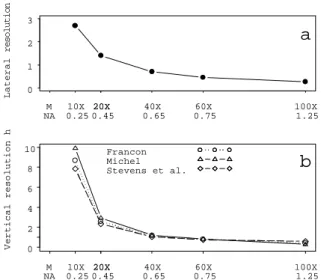
microscope) should be larger than the vertical resolution of the microscope. From the particle counting theory the term lost polar caps height is known, but its estimation has not been exactly defined. We propose that, instead of the lost polar caps height we calculate and use the vertical resolution (depth of focus = h) for a microscope objective with a defined numerical aperture as an approximation. If the contrast between the particles and the surroundings is not maximal, the height of lost caps is probably larger than the depth of focus, but a correlation between the lost polar caps height and the vertical resolution nevertheless exists (Fig. 1).
0 1 2 3
Lateral
resoluti
o
n
d
n
M 10X 20X 40X 60X 100X
NA 0.25 0.45 0.65 0.75 1.25
20X
a
0 2 4 6 8 10
Vertical resolutio
n
h
M 10X 20X 40X 60X 100X
NA 0.25 0.45 0.65 0.75 1.25
20X
b
Francon Michel Stevens et al.
Fig. 1. The relation between the magnification of the objectives 10× to 100× and (a) lateral resolution (d) in µm, calculated according to the equation of Abbe (Boyd, 1995) and (b) vertical resolution (depth of focus) of the microscope (h) in µm, calculated according to equations from Francon (1961) and Michel (1981) for the light microscope or Stevens et al. (1994) for the confocal microscope. Possible additional effect of the physiological eye accommodation has not been taken into account. M: objective magnification, NA: numerical aperture.
D
Fig. 2. In the reference space all the particles with
centres dislocated from the section plane for '
are included. For particles in reflected light the equation (1) NV = NA/D is used.
Wicksell (1925, 1926) expressed the classical stereological principle that the number of particle
profiles in the test area (NA) is proportional to the
numerical density (NV) of the particles and their
average tangent diameter (D), from which we deduce the following Eq. 1
NV = NA/D. (1)
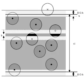
This principle could be used for particle counting in reflected light (Fig. 2). But in biological objects we usually observe and count particles in slices of thickness (t) in transmitted light. The thickness of physical slices (called also sections) is usually 0.05 0.08 µm for ultrathin sections, 0.5 - 2.0 µm for semithin sections, 5 – 10 µm for normally thick sections and several tens to over 200 µm for thick sections. The section can be thick or thin. In thick sections we can count particles in the whole slice thickness by successively turning the micrometer screw from top to down in order to see clearly the particles at all depths (Fig. 3). In both thin and thick sections, we have to take into account, besides the Wicksell's principle, corrections for slice thickness (t) and lost polar caps (h), according to Eq. 2 developed by Agduhr (1941), Floderus (1944) and Abercrombie (1946):
NV = NA/(t + D – 2h). (2)
t h
D/2-h D/2-h
t+D-2h
Fig. 3. Particles inside the height (t+ D – 2h) belong to the reference space of a thick section with the height t and NV = NA/(t + D – 2h).
The smallest usable slice thickness is the optical section thickness with height h (Fig. 4). In this case we count the particles at the level of the optical section
without moving the micrometerscrew.
D/2-h D/2-h
D-h h
Fig. 4. The particles with the centres inside space with the height (h + D – 2h) = D – h belong to the reference space of the thinnest optical section with the vertical resolution h.
Using the method for differential counting according to Ebbeson and Tang (1965) we take two
physical sections of differing thicknesses (t1 > t2),
count the particles per test area in each of them (NA1
and NA2) and calculate the numerical density according
to Eq. 3
NV = (NA1 – NA2)/(t1 – t2), (3)
for which knowledge of the particle diameter is obviously not necessary.
t1 h
D/2-h D/2-h
h
Fig. 5. Using the method for modified differential counting we count first the particles seen in one thick section (NAt) and then in one thin optical section of thickness t = h inside the same physical section (NAh). Equation NV = (NAt – NAh)/(t – h) is used.
The above procedure can be simplified by counting particles within a thick slice, and by taking an optical section inside of the thick physical section instead of a thinner physical section (Pajer and Kališnik, 1984; Kališnik and Pajer, 1985) (Fig. 5), leading to the Eq. 4
NV = (NAt – NAh)/(t – h). (4)
In all cases above the reference space is limited by two planes but is open above and under the real space, extended in both directions by a virtual space. Limiting the reference space also from above by a third forbidden plane (Fig. 6) we obtain two disector methods, for physical sections (Sterio, 1984) and for optical sections (Howard et al., 1985). In the physical disector method we cut the object into pairs of sections, the one being the forbidden or control section, and the other used as counting or reference section. We do not count particles in the forbidden section (look-up section). Additionally, in the counting section we do not count particles, which are seen also in the forbidden section. We count particles, which are seen in the counting section only. But since the reference space of the second, counting section, is reduced from above for the thickness of the »shadow« from the first, control section, (i.e. the lower virtual space of the first section), it is augmented under the real space for the same thickness (i.e. the lower virtual space of the second section). The final slice thickness is thus equal to the physical section thickness t (Fig. 7a, b). The Eq. 5 for this method is simply
NV = NAt / t, (5)
as has been published by Collan (1991).
& '
% $
* +
) (
)
D/2-h t
a
D/2-h
t D/2-h
t
b
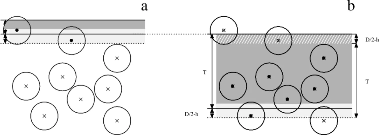
Fig. 7 a, b. Physical disector: The particles with centres in the lower virtual space of the forbidden paired section (a) with height (D/2 – h) are not counted in the reference section (b).
In the reference section we do not count the particles with the centres inside the part of the upper virtual space which is in the »shadow« of the forbidden paired section. The final reference space of the counting section has the height (t + D/2 – h) – (D/2 – h) = t.
Theoretically this method would be ideal and superior to all former methods. In reality its application is much more demanding and the results are less reliable than those of the older methods. It is necessary to cut exact series of pairs of sections and to mount each first section on one slide and each second on the other slide, marking them to indicate they are a pair, in order to match them perfectly. Further, additional equipment is necessary in form of a tandem projection microscope, or two microscopes each with its own digital camera and own videomonitor or one microscope with motor driven stage, one camera and a monitor. Ignoring the additional costs for equipment and tedious preparation of pairs of sections, the results of this method are uncertain because of possible mistakes in identification of particles, occurring in
both sections (look-up and counting), this error being additive in each pair of sections.
Some of these problems in using the physical disector method are avoided by the use of the so-called optical disector method. This method is actually an improved method for thick sections, with the reference space delimited with three forbidden planes (Fig. 8a, b). This method can also be performed, under favourable conditions, in the common optical microscope, though the use of a confocal microscope is recommended. But, one constraint remains: in counting particles, not only those seen in the forbidden optical section have to be ignored but also those seen in the first counting optical section, if they have been seen in the forbidden section. Otherwise this method becomes simply the method for thick sections.
D/2-h t
a
D/2-h T
D/2-h
T
b
Fig. 8 a, b. Optical disector: The particles with centres inside the lower virtual space of the forbidden upper optical section (a) are not counted in the first counting optical section (b).
The aim of the present study is to verify the hypothesis that all enumerated methods for numerical density estimation give accurate results if all necessary conditions are assumed and properly respected and if the sample is representative and large enough. In addition, we shall compare the efficiency and robustness of all the methods using the computer simulation as well as geometrical and mathematical analysis. We shall conclude by summarizing the feasibility of some of the above methods.
COMPUTER SIMULATION AND
MATHEMATICAL ANALYSIS
For each type of methods for estimation of particle number we have used a computer simulated counting process. Particles with selected diameter D = 7 µm were counted in a model object of nearly 4000 nonoverlapping particles in a cube of 300 µm edge
with a particle density NV = 145296 mm
-3
. Particles were treated as spheres with diameter D, with minimal distance between the particle centres being 2D = 14 µm. The model object was generated in two phases. First, a large number uniformly distributed points in 3-dimensional space was generated. In the next step, points with minimal distance to other points smaller than 2D were eliminated. The remaining points represent particle centres of nonoverlapping spheres.
To avoid problems with border space, the actual model space was enlarged in each dimension by D. To select a slice, the vertical position of a slice was selected at random. Slices with thicknesses 0, 0.5, 1, 2.5, 5, 10, 25, 50, and 100 µm were generated. On each slice, the random sample of n = 10 test areas was
taken. For each area the particles meeting the criteria of the particular estimation method were counted and used in the appropriate formula for particle density estimation.
The counting process was repeated m = 10 times, giving m estimates for the particle density. Standard deviation of m estimates was used as standard error (SE) and mean value of m estimates was taken as the
particle density estimate (
N
V'
) for a particular method. The standard deviation s for a sample of test
areas was estimated from SE as
s
=
SE
⋅
n
.Accuracy
Accuracy was described by the relative standard error
RSE = SE / NV , (6)
and relative error of estimate
RE
=
(
N
V−
N
V) /
N
V' (7)
Efficiency
To measure efficiency, the required number of test
areas (nreq) and total number of counted particles
(Creq), required for RSEreq = 5% were estimated from
simulated estimates:
n
s
N
RSE
req
V req
=
⋅
2
(8)
C
req=
n
req⋅ν
(9)where s is the standard deviation and
ν
the averagenumber of particles per area counted in the simulation.
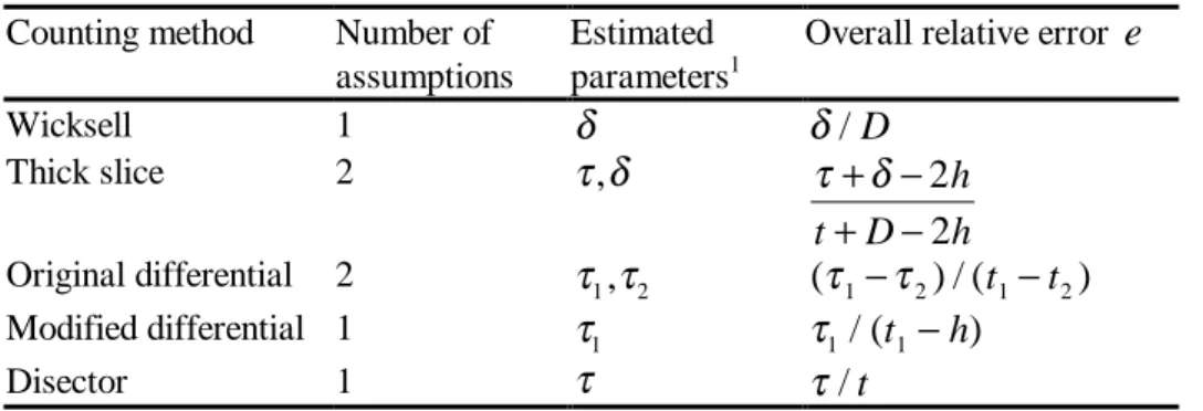
Table 1. Overall relative error e for various counting methods.
Counting method Number of
assumptions
Estimated
parameters1
Overall relative error
e
Wicksell 1
δ
δ
/ D
Thick slice 2
τ δ
,
τ δ
+ −
+ −
2
2
h
t
D
h
Original differential 2
τ τ
1,
2(
τ τ
1−
2) / (
t
1−
t
2)
Modified differential 1
τ
1τ
1/ (
t
1−
h
)
Disector 1
τ
τ
/ t
1
δ
Robustness
Robustness was described by the relative error of estimate. It depends on the number of assumed parameters and the relative error of estimate of each parameter. In general, the overall overestimate of
parameters (e.g. particle diameter
D
and slicethickness
t
) leads to an underestimate of particlenumber and vice versa. The relative error of particle
density RE’ = – e / (1 + e) where
e
is the overallrelative error of the parameter estimate given in Table 1.
Feasibility
Feasibility was evaluated qualitatively.
RESULTS
Results are presented under Accuracy, Efficiency and Robustness. Feasibility is considered in the Discussion.
Accuracy
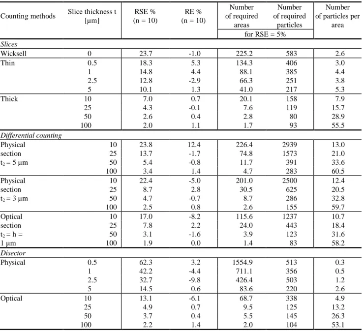
The values for relative standard error RSE and relative error of estimate RE, as criteria of accuracy, are presented in Table 2 and Fig. 9. In all methods, with increasing slice thickness, both parameters decrease
and the estimates approach the true value NV.
Table 2. Results of computer simulation presenting relative standard error (RSE), relative error (RE), number of areas and number of counted particles required for RSE = 5%, and the corresponding number of particles per area for various counting methods and slice thicknesses (t).
Counting methods Slice thickness t [µm]
RSE % (n = 10)
RE % (n = 10)
Number of required
areas
Number of required
particles
Number of particles per
area for RSE = 5%
Slices
Wicksell 0 23.7 -1.0 225.2 583 2.6
Thin 0.5 18.3 5.3 134.3 406 3.0
1 14.8 4.4 88.1 385 4.4
2.5 12.8 -2.9 66.3 251 3.8
5 10.1 1.3 41.0 217 5.3
Thick 10 7.0 0.7 20.1 158 7.9
25 4.3 -0.1 7.6 119 15.7
50 2.6 0.4 2.8 80 28.9
100 2.0 1.1 1.7 93 55.5
Differential counting
Physical 10 23.8 12.4 226.4 2939 13.0
section 25 13.7 -1.7 74.8 1573 21.0
t2 = 5 µm 50 5.4 -0.8 11.7 391 33.6
100 3.4 1.4 4.7 283 60.5
Physical 10 22.4 -5.0 201.0 2500 12.4
section 25 8.7 2.8 30.5 625 20.5
t2 = 3 µm 50 4.7 -0.7 8.7 286 32.8
100 2.5 0.8 2.6 155 59.7
Optical 10 17.0 -8.2 115.6 1237 10.7
section 25 7.8 2.2 24.0 443 18.4
t2 = h = 50 3.1 -1.6 3.9 123 31.6
1 µm 100 1.9 0.0 1.4 83 58.2
Disector
Physical 0.5 62.3 3.2 1554.9 513 0.3
1 42.2 -4.4 711.1 356 0.5
2.5 32.7 -9.8 426.4 503 1.2
5 14.5 0.6 83.6 220 2.6
Optical 10 13.1 -6.1 68.7 338 4.9
25 4.9 0.7 9.5 125 13.2
50 3.7 0.4 5.5 145 26.3
Slice thickness t [µm] 0. 0 0. 5 1. 0 1. 5 2. 0 R e la ti v e n u m b e r of par ti c les
0 10 25 50 100
a
-10% Nv +10%
Slice thickness t [µm]
0. 0 0. 5 1. 0 1. 5 2. 0 R e la ti v e n u m b e r of par ti c les
0 10 25 50 100
b
-10% Nv +10%
Slice thickness t [µm]
0. 0 0. 5 1. 0 1. 5 2. 0 R e la ti v e n u m b e r of par ti c les
0 10 25 50 100
c
-10% Nv +10%
Thin slice thickness t` [µm]
0. 8 0. 9 1. 0 1. 1 1. 2 R e la ti v e n u m b e r of par ti c les
0 1 3 5
d
-10% Nv +10%
Fig. 9. Accuracy of different particles counting methods estimated by the relative number of particles indicated by 95% confidence intervals (vertical bars) and averages (
ο
) at various slice thicknesses t for a classical thin and thick slices, b physical and optical disector, c modified differential counting (t2 = h), and d differential counting with t1 = 100 µm and different t2 (1, 3, 5 µm).Efficiency
The values for the required number of areas nreq
and required number of counted particles Creq in order
to obtain RSE = 5% as criteria for efficiency
0.5 1 5 10 50 100 Slice thickness [µm]
1 10 100 100 0 N u m ber of ar eas Slice Disector Differential counting: t`=1µm t`=3µm t`=5µm
a
are presented in Table 2 and Fig. 10. In general, with increasing slice thickness both parameters decrease and converge to similar values regardless of the counting method.
0.5 1 5 10 50 100 Slice thickness [µm]
50 100 500 100 0 500 0 N u m ber of pa rt ic le s Slice Disector Differential counting: t`=1µm t`=3µm t`=5µm
b
Robustness
The values for the relative error of the estimated particle density RE’ for under- and overestimated particle diameters for different slice thicknesses for the classical and modified differential method are presented in Fig. 11. Fig. 12 shows RE’ for under- and overestimated slice thicknesses and for combination of under- and overestimated particle diameter and slice thicknesses for various counting methods. In general robustness increases with increasing slice thickness.
0 20 40 60 80 100 Slice thickness [µm]
-3 0 -2 0 -1 0 0 10 20 30 R e la ti v e e rr o r [% ]
Thick slice: t
a -2 -1 -0.5 0 0.5 1 2
0 20 40 60 80 100 Slice thickness [µm]
-3 0 -2 0 -1 0 0 10 20 30 R e la ti v e e rr o r [% ] Differential: t1 b -2 -1 -0.5 0 0.5 1 2
Fig. 11. Robustness of different particles counting methods estimated (a) by relative error of estimated particle density in classical counting methods for underestimated (-1, -2, -3 µm) or overestimated (+1, +2, +3 µm) particle diameters D at various slice thicknesses and (b) by the relative error of estimated particle density in modified differential method for underestimated (-0.5, -1, -2 µm) or overestimated (+0.5, +1, +2 µm) slice thicknesses t1 at various true slice thicknesses.
0 20 40 60 80 100
Slice thickness [µm]
-30 -20 -10 0 10 20 30 R e la ti v e e rr o r [% ] Differential Disector Thick slice
τ = -1µm
τ = +1µm
a
0 20 40 60 80 100
Slice thickness [µm]
-30 -20 -10 0 10 20 30 R e la ti v e e rr o r [% ] Differential Disector Thick slice
τ,δ = -1µm
τ,δ = -1µm
b
Fig 12. Robustness of different particles counting methods estimated by the relative error of estimated particle density (a) for underestimated (-1 µm) or overestimated (+1 µm) slice thickness at various true slice thicknesses t and (b) for underestimated or overestimated particle diameter and slice thickness (both for ±1 µm) at various true slice thicknesses t.
τ: difference between false and true slice thickness,
δ: difference between false and true particle
DISCUSSION
Assumptions
are indispensable in scientific workbut they have to be logically and/or empirically verified. In all cases we expect a certain precision of the estimates.
In transmission light microscopy we always observe particles in optical sections with the true thickness h of the vertical resolution corresponding to certain objective magnification and its numerical aperture, if the thickness of the physical slice is equal or larger, which usually holds for normally thick slices. If the physical slice is thinner than the optical section, which can be the case in semithin slices, the physical slice thickness is the true thickness in which we observe the particles. If we observe particles in several successive optical sections, we can proceed to the real physical slice thickness t. We have to measure or calculate the corresponding section or slice thickness t.
In counting procedures we have to define the reference space. If we adhere to the rule of the particle associated point in counting procedures there is no limitation in applying any of the above six analyzed counting methods regardless the form, size and possible orientation of the particles. In classical counting methods for thin and thick slices two forbidden planes and two permitted planes laterally delimit the reference space. The reference space is augmented with a virtual space of the thickness D/2 - h above and under the true slice, and the total reference space amounts to t + D – 2h in vertical dimension. In this case we have to deal with two additional assumptions, about the vertical height of particles and about the height of lost polar caps. The vertical height of particles can be measured and/or calculated, which can be an uncertain and sometimes complicated procedure. However, for the vertical height of the lost polar caps the vertical objective resolution h can be used as the best possible approximation.
In both disector methods, the reference space is delimited with three forbidden and three permitted planes. There is no need to know either the height of particles or the height of lost polar caps. So we only have to measure the real slice thickness.
In the original differential counting method (Ebbeson and Tang, 1965) we have to measure the
thickness of the thicker (t1)and thinner (t2) slice. In the
modified differential counting method (Kališnik and Pajer, 1985) only one assumption is necessary, i.e. the thickness t of the thicker slice; thickness of the thinner slice is simply vertical objective resolution h. In this case the situation is similar to that of the disector methods.
The disector methods were declared in 1984 as being highly efficient, unbiased design based and assumption free methods. According to the protagonists of these methods all the older methods for particle counting should be abandoned (Mayhew and Gundersen, 1996; Dorf-Petersen et al., 1998). In the majority of cases these methods have been applied uncritically. Only a few critical approaches have been made to date (DeGroot and Bierman, 1986; Kališnik et al., 1987; Calverly et al., 1988; Popken and Farel, 1996, 1997; Tramontin et al., 1998; Hedreen, 1998a, 1998b; Hatton and Bartheld, 1999; Bartheld, 1999; Collan, 1991, 1999).
The physical disector method appears to be a good solution for particle counting in electron microscopy, but the situation is quite different in light microscopy. Therefore we have resumed our comparison of some older counting methods with the disector methods.
We have confirmed our first hypothesis, that all six methods give valid and accurate results, if the sample is representative and large enough. In this respect there is no difference between these methods.
Other expectations concerning the differences in efficiency, robustness and feasibility have also been confirmed. Efficiency can be defined as the ratio between the inverse value of standard error and the square root of the time necessary for performing counting. Since time in computer simulation cannot be measured, we have calculated the number of areas and number of counted particles at certain standard errors necessary to obtain RSE = 5%. There is an evident increase of efficiency with increasing slice thickness in all three pairs of methods. In classical method, therefore, the thick slices are superior to thin slices, the modified differential counting is superior to the original differential counting method and the optical disector method is superior to the physical disector method, as regards their efficiency.
disector methods, it could be expected, that the latter would be more robust. We have tried to check the robustness by the introduction of false data for assumptions for particle height, for slice thickness and for combination of the two. It can be seen that robustness is superior in both differential and disector methods. Besides, the robustness can be judged also from the standard error at different slice thicknesses. It also obviously increases with the slice thickness.
Feasibility can be judged according to the additional equipment and additional procedures necessary for performing certain counting methods. It is obvious, that the physical disector method is least feasible, because the demanding and risky pairing of slices and particles is necessary and because additional equipment is necessary, e.g. tandem projection microscope, or two microscopes, each with its own digital camera and own videomonitor or one microscope with motor driven stage, one camera and monitor. The classical methods for thin and thick slices are also less feasible because they need initial particle caliper diameter estimation what may be time consuming and not reliable.
The results of our computer simulation study are directly valid only for the model of randomly distributed spheres. But, it could be speculated, that similar results would be obtained also for any form, size and orientation of particles, since the particles associated points have been counted. So the conclusions of our study could be generalized after empirical verification.
In practice the counting of particles through the entire thickness of a physical slice is arguable since the identifiability of particle fragments in the upper and lower faces of a slice is questionable. The problems are overcome by operating inside a reasonably thick slice, avoiding its physical lower and upper bounding faces. One can regard our model as such limited space within thicker physical slice. However, it is evident that not all practical problems can efficiently be solved with models.
REFERENCES
Abercrombie M (1946). Estimation of nuclear population from microtomic sections. Anat Rec 94:239-47.
Agduhr E (1941). Beitrag zur Technik fuer die Bestimmung der Anzahl Nervenzellen je Volumeneinheit Gewebe. Anat Anz 91:70-81.
Bartheld CS (1999). Systematic bias in an »unbiased« neuronal counting technique. Anat Rec 257:119-20.
Boyde A. Confocal microscopy (1995). In: Wotton R, Springall DR, Polak JM (eds). Image analysis in histology: conventional and confocal microscopy. Cambridge: Cambridge University Press, 151-96. Bodziony J, Wiencek K, Rys J. (1998). A survey on NV
stereology for convex particles in metallography. Acta Stereol 17:143-55.
Calverly RKS, Bedi KS, Jones DG (1988). Estimation of the numerical density of synapses in rat neocortex. Comparison of the »disector« with an »unfolding« method. J Neurosci Meth 23. 195-205.
Collan Y (1991). Quantitative histopathology of soft tissue calcifications. Proc Finn Dent Soc 87:643-50.
Collan Y (1999). The Ebbeson-Tang formula. Theoretical background of an alternative to the disector in stereological cell counting studies. Anal Quant Cytol Histol 21:147-50.
Dorph-Petersen KA, Nyengaard JR, Gundersen HJG (1998). A brief introduction to particle number estimation. Acta Stereol 17:201-14.
DeGroot DM, Bierman EP (1986). A critical evaluation of methods for estimating the numerical density of synapses. J Neurosci Meth 18:79-101.
Ebbeson SOE, Tang D (1965). A method for estimation the number of cells in histological sections. J R Microsc Soc 84:449-64.
Floderus S (1944). Untersuchungen ueber den Bau der menschlichen Hypophyse mit besonderer Beruecksichtigung der quantitativen mikromorpho-logischen Verhaeltnisse. Acta Path Microbiol Scand Suppl 53.
Francon M (1961). Progress in microscopy. Evantson (Illinois): Row, Peterson.
Hatton WJ, von Bartheld CS (1999). Analysis of cell death in the trochlear nucleus of the chick embryo: calibration of the optical disector counting method reveals systematic bias. J Comp Neurol 409:169-86. Hedreen JC (1998a). Lost caps in histological counting
methods. Anat Rec 250:366-2.
Hedreen JC (1998b). What was wrong with the Abercrombie and empirical cell counting methods? A review. Anat Rec 250:373-80.
Howard V, Reid S, Baddely A, Boyde A (1985). Unbiased estimation of particle density in the tandem scanning reflected light microscope. J Microsc 1138; 203-12. .DOLãQLN 0 ,OLü 0 /X]DU $ 3DMHU = 7KH
importance of section thickness and particle diameter ratio in number per unit volume estimation evaluated by computer simulation (Preliminary report). Acta Stereol 6/Suppl II:193-202.
Mayhew TM, Gundersen HJG (1996). »If you assume, you can make an ass out of u and me«: a decade of the disector for stereological counting of particles in 3D space. J Anat 188:1-15.
Michel K (1981). Die Grundzuege der Theorie des Mikroskops. 3. Auflage. Stuttgart: Wissenschaftliche Verlagsgesellschaft.
P ajer Z , K ališn ik M (1 9 8 4 ). T h e particle n u m ber estim ation an d th e d epth of focu s. A cta S tereol 3 :1 9 -2 2 .
Popken GJ, Farel PB (1996). Reliablity and validity of the physical disector method for estimation neuron number. J Neurobiol 31:166-74.
Popken GJ, Farel PB (1997). Sensory neuron number in neonatal and adult rats estimated by means of stereologic and profile-based methods. J Comp Neurol 386:8-15.
Stevens JK, Mills LR, Trogadis JE (1994). Three-dimensional confocal microscopy: Volume
investigation of biological systems. San Diego: Academic Pres, Inc.
Sterio DC (1984). The unbiased estimation of number and sizes of arbitrary particles using the disector. J. Microsc 134:127-36.
Tramontin AD, Smith GT, Breuner CW, Brenowitz EA (1998). Seasonal plasticity and sexual dimorphism in the avian song control system: stereological measurement of neuron density and number. J Comp Neurol 396:186-92.
Weibel ER (1979). Stereological methods. Practical methods for biological morphology. London etc.: Academic Press.
Wicksell SC (1925). The corpuscle problem I. Biometrica 17:84-99.