Accounting for the Effects of Mortality Selection Bias on Health Outcomes: A
Case Study of the Great Chinese Famine
By: Alice Huang
Honors Thesis Economics Department
The University of North Carolina at Chapel Hill
April 2016
Approved:
2 Acknowledgements
I would like to thank my thesis advisor Dr. Klara Peter for her endless support, patience, and contributions to this project. I am especially grateful to Dr. Peter for her willingness to share her expertise and passion for research, for the countless Friday mornings she spent mentoring me, and for challenging me to produce a final project I can be proud of. I could not have done this without her support.
Additionally, I would like to thank Hsi-Chu Bolick and Ai-Ling Chang in the East Asian Studies Department for their endless help finding primary sources on famine and referring me to the appropriate resources. I would also like to thank the Morehead-Cain Foundation for enabling me to travel to China over the Winter Break to study the institutional details of famine in Guangxi Province and visit several archives.
3 Abstract
Using individual-level variation in famine exposure and intensity based on individual
month-year-region of birth and historical data on the size of narrowly-defined birth cohorts,
I find that exposure to famine negatively impacts adult height, lowers BMI, negatively
affects health status, and reduces incidence of serious illness and hypertension. I use
Inverse Probability Weighting and Joint Modeling of Longitudinal and Survival Data to
account for selective mortality bias in health outcome equations. Contributions are mainly
threefold: first, I exploit individual-level variation in timing and length of exposure, which
serves as a more precise proxy for famine. Secondly, I include additional health variables
into my analysis. Finally, I apply innovative techniques to account for selective mortality
4 1. Introduction
Longitudinal studies and research questions regarding the effects of exogenous factors on
the evolvement of longitudinal responses have become increasingly popular among researchers.
However in order to produce consistent estimates in the context of these studies, researchers need
to address and account for potential attrition bias.1
In this study, I am interested in measuring the causal effects of the Great Chinese Famine
of 1959-61 on later-life health outcomes. I use the Chinese Health and Nutrition Survey (CHNS)
and census data from the Integrated Public Use Microdata Series-International (IPUMS-I) to
capture the effects of the famine on the evolvement of health responses over time. However, since
observed and unobserved factors may underpin both the health indicators of interest and selection
into participation (i.e. individuals with poor observed health outcomes are more likely to die before
subsequent rounds), such losses may induce selective mortality bias on the health estimates.
Suppose I fail to account for selective mortality bias. In the panel, I only observe subjects
who “survived” a process in the analysis. As a result, in each subsequent survey round, I observe
respondents with better initial health stocks. Since the dependent variables of interest are health
variables and the characteristics of likely death (i.e. poor health, frailty) are correlated to health
outcomes, failing to account for selective mortality bias could produce inconsistent estimates of
the true impacts of the famine.
The Great Chinese Famine of 1959-61 provides a useful case study for the effects of
selective mortality bias on later-life health outcomes. Viewed as one of the worst human
catastrophes of the 20th Century, the famine is estimated to have caused upwards of 45 million
1 All surveys lose respondents, but if selection occurs in a non-random manner, namely if individuals with similar
5
excess deaths and led to persistent health and nutritional deficiencies for survivors (Gorgens et al.,
2012; Lin and Yang, 1998).2 The Chinese famine literature is comprehensive; researchers have
studied the impact of the Chinese famine on various later-life health outcomes including height,
obesity, and incidences of chronic disease. However as far as I can tell, no study has attempted to
correct for the effects of selective mortality bias on these health estimates.
Furthermore, there is large interest in examining how the effects of early childhood shocks
persist and impact later-life health outcomes. Economic theory has posited the “critical period
hypothesis” in which shocks in utero and early childhood have disproportionate effects on
later-life outcomes (Heckman, 2007; Almond and Currie, 2011a and 2011b). In this paper, I attempt to
improve upon previous studies of the effects of early life exposure to famine and determine the
mechanisms by which shocks in utero and early childhood have persistent effects on adult health
outcomes. Contributions of this study are primarily three-fold. First, using historical birth cohort
data, timing, and place of birth, I exploit individual-level variation in timing and length of famine
exposure. As such, not only do I examine the effect of famine exposure on my vector of health
outcomes, but also the effects of age of exposure and length of exposure. Secondly, I include
additional health variables, including health index and incidence of serious illness, and offer
comparisons for the effects of famine across these health indicators. Finally, I account for selective
mortality bias using Inverse Probability Weighting and Joint Modeling techniques and revise
previous estimates in the health equation. In particular, I show how these methods can be used to
account for selective mortality bias in future longitudinal studies. Limitations of this study include
failure to account for selection into survival at the time of the famine, which may counter the
observed adverse effects of famine on later-life health outcomes.
2 Excess mortality estimates range from 16.5 million (Coale, 1981) to 30 million (Banister, 1987) to 45
6
I find that exposure to famine does negatively impact adult height, lower BMI, negatively
affect health status, and reduce incidence of serious illness and hypertension. In particular, I find
that within the critical period, older ages of famine exposure cause more significant declines in the
health index. Furthermore, while IPW and Joint Modeling estimations suggest though the baseline
health estimates are biased, individuals exposed to famine are less likely to die, which indicates
the selection effects may confound the adverse effects of famine.
The paper will proceed as follows. Section 2 provides greater context for the Great Chinese
Famine and summarizes the existing literature regarding the Chinese Famine and selective
mortality bias. Section 3 details the theoretical model, and Section 4 describes the data. The
empirical strategy for my baseline health equation and the baseline health results are presented in
Section 5. Section 6 discusses the selective mortality issue and provides the empirical framework
for IPW and Joint Modeling. Results from the IPW and Joint Modeling estimation methods can be
found in Section 7. Section 8 discusses, and Section 9 concludes.
2. Background and Related Literature
2.1 The Great Chinese Famine
The extent, nature, and effects of the Great Chinese Famine have been a source of
widespread fascination among researchers. Earlier studies have focused on the causes of
the famine and its effects on childbearing behavior (Peng, 1987; Lin and Yang, 2000).
Newer studies examine the long-term health and economic consequences of the famine
among survivors and children born during the three-year period of the famine. The
emerging Chinese famine literature predominately offers empirical support for the growing
literature on the effects of early-life shocks on later-life outcomes. Chen and Zhou (2007)
7
taller in adulthood. Similar studies have found that exposure to famine in early childhood
has adverse effects on height, obesity, and mental health (Gorgens et al., 2012; Fung, 2009;
Almond et al., 2010; St. Clair et al., 2005).
The Chinese famine literature is also closely related to other contexts in which
unexpected and disastrous events, such as wars and famines, are experienced early in life.
Using the context of the Nigerian Civil War of 1967-70, Akresh (2011) finds that exposure
to war at any time between birth and adolescence reduced adult stature and thereby reduced
life expectancy and adult earnings. Lee (2014), in studying the long-term effects of the
Korean War (1950-53), finds that the war had the largest adverse effect on the educational
attainment and labor market performance on individuals who were in utero during the worst
time of the war.
In studying the effects of the Great Chinese Famine on adult outcomes and
establishing causal linkages, previous studies have used various measures of famine
intensity. Previous proxies for famine include province-level annual excess death rates
(EDR) in 1959-613 (Shi, 2007), province-level annual EDR in 1960 (Chen and Zhou,
2007), and county-level annual size of surviving cohort (Meng and Qian, 2006, 2009).
These proxies allow researchers to capture cross-sectional variation in famine intensity
across regions and birth cohorts. However to my knowledge, no study uses individual-level
variation in famine exposure and intensity based on individual month-year-region of birth
and historical data on the size of narrowly-defined birth cohorts.
The CHNS has also been widely used for studying the persistent effects of the Great
Chinese Famine on later-life health and economic outcomes. However, many studies rely
3 Excess death rate in 1959-61 (1960) is defined as the difference between the crude death rate (CDR) in
8
on cross-sectional data from a single round of the survey.4 In contrast, I am interested in
the longitudinal aspects of health outcomes and employ all existing rounds of the CHNS.5
In addition, previous studies use various empirical strategies to test the effects of
famine on later-life outcomes. Several studies use a two-period, two-group
difference-in-difference analysis6 while other studies implement cohort analysis.7 Finally, studies in the
Chinese famine literature address sources of sample selection bias. Gorgens et al. (2012)
and Meng and Qian (2010) use different techniques to address the issue of positive
selective for survival.8 However as far as I can tell, no study has attempted to address the
issue of selective mortality bias on health estimates.
2.2 Selective Mortality Bias
In studying the effects of the Great Chinese Famine on later-life health outcomes,
I ask: does selective mortality matter, and will it produce biased estimates in the health
equation? Selective mortality bias is a form of attrition bias. Hence, I draw from the
literature detailing the impacts of attrition on longitudinal studies. In the case of
4 Meng and Qian (2006), using the 1989 survey, find that individuals who were exposed to famine during
early childhood have a lower weight by 5% in comparison to those who were not exposed; Chen and Zhou (2007) use the 1991 survey to study the effects of famine on later-life economics consequences.
5 Other studies implement the longitudinal aspect of the CHNS: Luo et al. (2006), using rounds from 1991 to
2000, finds that famine exposure increases the probability of being overweight for women in rural areas. Similarly, Gorgens et al. (2007) uses the 1989, 1991, 1993, and 1997 surveys to study the stunting and selection effects of famine on adult height.
6 Several studies use a DID empirical strategy: Luo et al. (2006) compares the effects of famine between
those born in 1959-62 to those born in 1963-66; Meng and Qian (2006) defines the treatment group as those born in 1952-54, 1955-58, and 1959-60 and the control group as those born in 1961-64; Chen and Zhou (2007) compares those born in 1954-62 to those born in 1963-67.
7 Other studies implement cohort analysis: Almond et al. (2007) conducts within-cohorts comparisons for
those born in 1956-64; Gorgen et al. (2007) divide the treatment group into the “old” famine cohort (those born in 1948-56) and the “new” famine cohort (those born in 1957-61).
8 Gorgens et al. (2012) disentangles the stunting and selection effects of famine by comparing the heights of
9
random attrition, losses in subsequent rounds may induce sample selection bias (Gerry and
Papadapoulos, 2013). Since mortality is correlated to my observed health outcomes and
therefore non-random, not accounting for selective mortality bias could bias the health
estimates.
Particularly in regards to my dependent variables of interest, the importance of
correcting for selective mortality bias is highlighted in comparisons of the effects of
attrition due to death and attrition due to other causes. Weuve et al. (2013) find larger and
more significant effects when correcting for survivorship bias9 than when correcting for
attrition bias due to other causes. This finding indicates that selection mortality does cause
a fundamental shift in the underlying population from one survey round to the next, and
this difference is heightened over time.
The literature also highlights several approaches to addressing selective mortality
bias. One possible method, particularly salient in the epidemiological literature, is Inverse
Probability Weighting (IPW). Under IPW, users essentially re-weight their estimates to
account for observed non-random attrition. Gerry and Papadapoulos (2013), find
systematic health related attrition in the Russian Longitudinal Monitoring Survey by
finding a statistically significant difference in the weighted and unweighted pooled
estimates. Weuve et al. (2013) similarly uses IPW to address the methodological challenges
of the longitudinal effects of smoking on cognitive decline and finds that the unweighted
analysis underestimates the impact of smoking. Similarly, exposure to the Great Chinese
Famine may increase an individual’s likelihood of death through multiples rounds of the
CHNS and thereby underestimate the effects of famine.
10
Another possible method highlighted by the literature is the Joint Modeling
technique. This technique enables researchers to jointly model survival and longitudinal
processes (Crowther, Abrams, and Lambert, The Stata Journal). Previously, researchers
estimated survival and longitudinal measures separately using the random effects model
and Cox proportional hazard models (Ratcliffe et al., 2004). However, given that
longitudinal and survival processes are often related through unobserved characteristics,
separate models can result in biased estimates. As a result, joint modeling has become
increasingly popular. Guler et al. (2014) use this technique in an application to liver
transplantation data and find that for non-diabetic patients, longitudinal glucose levels have
a significant effect on survival. Similarly, I seek to estimate the direct and indirect effects
of famine exposure on mortality by way of longitudinal health responses.
Through implementing IPW and Joint Modeling techniques, I am able to produce
less biased health estimates. Differences between weighted and unweighted estimates will
confirm the presence of selective mortality bias and enable me to revise previous estimates
of the impact of famine on health outcomes.
3. Theoretical Model
Since I am interested in understanding the mechanisms by which early life shocks
affect later-life outcomes, I draw upon the conceptual framework from the “early
influences” literature in which shocks in utero and early childhood have persistent effects
on later-life health outcomes either directly through the biological effect or indirectly
11
To illustrate these mechanisms, I adopt Heckman et al.’s (2015) human capital
model of health capital. I assume each family has two children: 𝜏 = {𝑖, 𝑗}. The health
production function for child i in family k is therefore specified as:
𝜃𝑖𝑘 = 𝑓(𝜔𝑖𝑘, 𝐼𝑖𝑘, 𝑒𝑖𝑘; 𝜗𝑖𝑘, ℎ𝑖𝑘), (1)
where 𝑒𝑖𝑘 is defined as a negative health shock affecting child i in utero and early
childhood. Child prenatal health endowments, parental health capital investments, and
child health capital are indicated by 𝜔𝑖𝑘, 𝐼𝑖𝑘, and 𝜃𝑖𝑘respectively. Furthermore, child and
parental characteristics such as gender and ethnicity are denoted by 𝜗𝑖𝑘 and ℎ𝑖𝑘
respectively (Heckman, 2007).
The occurrence of famine in utero or early childhood could affect later-life health
outcomes indirectly through affecting parental intra-household allocation decisions. For
instance, the presence of famine may cause parents to allocate more resources to the child
with the highest prenatal health endowments. This would negatively impact the health
capital of the other children in the family. I specify parental preferences as:
𝑈 = 𝑈(𝑐, 𝑙, 𝑞𝑖, 𝑞𝑗, (2)
where c is parental consumption, l is parental leisure time, and 𝑞𝑖 is the quality of child i,
which is a measure of child i’s prenatal health and cognitive endowments. The parental
budget constraint takes into account the price of health capital investment, parental wage
rates and time available, and non-labor income. Upon maximizing the utility function
subject to the budget constraint and production function, the optimal health capital
investment of type a in child i takes the following form:
𝐼𝑖𝑎∗
= 𝑔𝑎(𝜔
12
where pIis the price of the investment, w is the parental wage, and Y is the non-labor
income.
As seen from the above function, the optimal investment strategy depends on the
parameters in the health production function and whether parents display reinforcing or
compensating preferences. Suppose ceteris paribus, 𝜔𝑖 > 𝜔𝑗. In the case of reinforcing
preferences, parents invest more in child i. In contrast, parents who display compensatory
preferences are likely to allocate more health capital investment in child j, thereby
“compensating” for the larger negative effects of the health shock on child j. Parental
intra-household allocation decisions are important in the context of the Great Chinese Famine.
In conditions of extreme scarcity, reflected in the budget constraint function through
increased prices and decreased parental wages, the decision to invest in child i could mean
little to no investment in the health capital of child j, thus having a more negative effect on
the health capital formation of child j than in normal years.
Famine could also affect health capital directly through the biological effect,
namely through changes in the underlying health production function. For instance, famine
exposure in utero and early childhood may cause persistent frailty, thus fundamentally
changing the individual’s ability to transfer post-shock health investments into health
capital.
The total effect of an early life health shock of child i’s health capital formation can
therefore be decomposed as:
𝑑𝜃𝑖
𝑑𝑒𝑖 =
𝜕𝜃𝑖
𝜕𝑒𝑖+
𝜕𝜃𝑖
𝜕𝐼𝑖 ∙
𝜕𝐼𝑖
13
where the left-hand side denotes the total effect of the early life health shock and the two
terms on the right-hand side denote the biological and behavioral effects10 respectively. In
the case of famine, the biological effect is assumed to be negative; the sign of the behavioral
effect depends on whether parents display reinforcing or compensatory preferences. In the
case of compensatory preferences, famine exposure in early life may have an overall
positive effect on health capital if the magnitude of the biological effect if less than that of
the behavioral effect.
The theoretical literature also proposes the life cycle of health capital formation and
the processes by which the effects of health shocks in early child persist late in life.
Assuming the health production process is governed by multistage technology, inputs in
each stage produce health outputs in the next (Cunha and Heckman, 2007). Persistence in
health inputs on later-stage outcomes works through self-productivity and dynamic
complementarity. According to the principle of self-productivity, famine exposure in utero
and early childhood, by reducing the early life health stock, lowers the potential health
stock for subsequent periods. The principle of dynamic complementarity, which suggests
that health investments in each period reinforce each other, highlights the importance of
parental investments, especially in earlier periods.
These principles bring into question the impact of selection into survival at the time
of the famine on the effects of early life famine exposure on later-life health outcomes. In
order for a child to survive the famine, his early life health stock
q
must be above someminimum threshold, 𝜃𝑚𝑖𝑛. As seen above, this health stock is achieved through some
combination of higher health endowment and higher level of parental investment. Given
14
reinforcing parental intra-household allocation behavior, the principle of dynamic
complementarity suggests that increased health investments during and after the period of
the shock may sufficiently compensate for the adverse biological effects of famine on the
health production function. In such cases, due to famine’s effect on parental health
investments, exposure to and subsequent survival of famine may actually cause survivors
to display better later-life health outcomes than a general population that was not exposed.
In this study, I present the direct and indirect effects of famine on later-life health
outcomes. Through the theoretical model, I can begin to understand the mechanisms by
which exposure to famine in utero and early childhood affects later-life health outcomes.
4. Data
The data for this study are obtained from the Minnesota Population Center’s
Integrated Public Use Microdata Series-International (IPUMS-I) and the Carolina
Population Center’s China Health and Nutrition Survey (CHNS). The former data source
is used to construct the measure of famine and while the latter is used to link exposure to
famine with the health outcomes of interest.
IPUMS-I contains census microdata from around the world. Specifically in the
context of this study, I use historical birth cohort data across 29 Chinese provinces, which
is available on a monthly basis.
Designed to examine the effects of health, nutrition, and family planning policies
in China, the CHNS consists of nine waves spanning 1989 to 201111. Approximately
15,000 individuals (4,000 households) are surveyed in each wave. Furthermore, the data
15
contains key community and individual-level variables including health infrastructure,
education, and occupational status.
Sampled provinces in the CHNS include Guangxi, Guizhou, Heilongjiang, Henan,
Hebei, Hunan, Jiangsu, Liaoning, and Shandong and vary substantially in terms of
geography, economic development, and public resources. Five provinces are coastal while
the other three are inland. Furthermore in terms of living standards, Jiangsu, Liaoning, and
Shandong are among the richest while Guangxi and Guizhou are among the poorest (Chen
and Zhou, 2007). Furthermore in line with this study, these provinces experienced great
heterogeneity in famine intensity.12
4.1. Measure of Famine
I use IPUMS-I to construct the measure of famine intensity. IPUMS-International
contains monthly historic birth cohort data across Chinese provinces. For the purposes of
this study, I use birth cohort data from January 1953 to December 1967 to construct my
famine “treatment” indicator and measures of famine intensity.
I use three definitions of famine exposure (moderate, severe, and devastating) based
on the extent of the drop in birth cohort relative to the size of the reference birth cohort.
For each month and province, I calculate the percent difference between the given birth
cohort and the reference birth cohort, namely the average of the cohort size for the same
month and province from 1955-57. Furthermore, due to natural seasonal and monthly birth
cohort variation, I designate that famine occurs in a particular month and place if the size
12 Although I use province of birth to merge the IPUMS-I and CHNS datasets, province of residence at the
16
of the relative birth cohort faces a drop as great or greater in the previous month. This
allows me to account for natural volatility in birth cohort size when creating grades for
famine.
Hence, moderate famine is defined as a drop of 20%+ in birth cohort in a given
month, given that the previous month experiences a similar drop of 20% in relative birth
cohort; severe and devastating famine are defined as drops of 30%+ and 40%+ in birth
cohort respectively. Creating grades for famine exposure based on the extent of the drop in
relative birth cohort size allows me to compare the effects of intensity of exposure on my
health outcomes.
The determination of the 20%+, 30%+, and 40%+ drop offs in relative cohort size
is based on examining the distribution of the percent difference between the birth cohort
size at time t and the reference period. Graph A (Appendix) shows the kernel density of
the relative birth cohort size from 1958 to 1962.13 The majority of the distribution
experienced a negative percent difference. In addition, the drop off in relative cohort size
at 20% growth suggests that any percent change in birth cohort size between -20% and
20% may be due to natural birth cohort volatility. Hence, I begin my definitions of famine
“treatment” at a 20% drop in relative birth cohort size.
4.1.1 Justification for the Measure of Famine
In this study, I exploit a novel proxy for famine: “severe” famine occurred in a
specific month and province if it is the second of two consecutive months that experienced
a drop of 30%+ in relative birth cohort size. To justify this as a reasonable measure for
13 I do not include periods before 1958 and periods after 1962. This is because period before 1958 comprise
17
famine intensity, I compare the trends in relative birth cohort size per month across
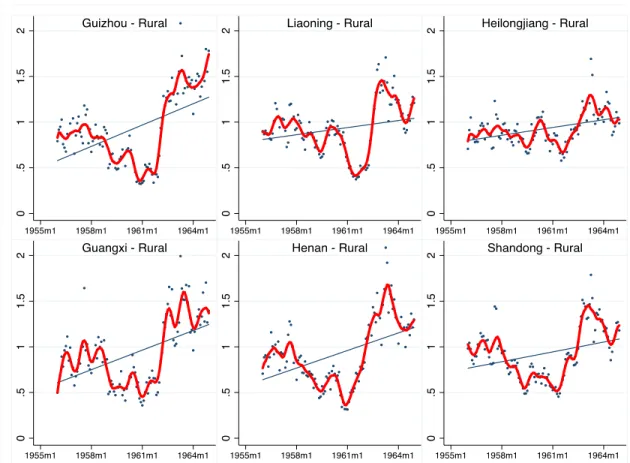
provinces. Figure 1 depicts the relative birth cohort per month across Guizhou, Liaoning,
Heilongjiang, Guangxi, Henan, and Shandong.14 Across these provinces, all experienced a
drop in relative birth cohort between 1958 and 1962. This time period corresponds with
the historical years of the Great Chinese Famine. It is also notable that the fitted line is
upward sloping, which indicates that the natural trend is increasing fertility across all
provinces. Hence, the departure from this natural trend gives further proof of a large
exogenous shock during this time period.
14 I conduct robustness checks for all provinces. All provinces experienced dips in relative birth cohort of
18
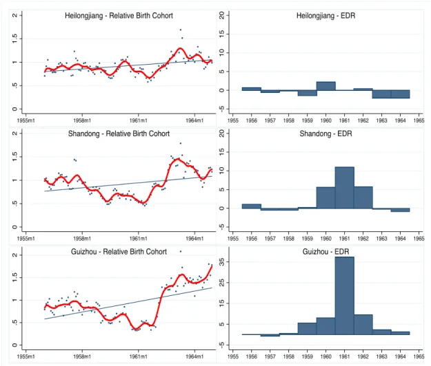
I also compare relative birth cohort size to excess death rates (EDR).1516 From
Figure 1, in order to validate relative birth cohort size as a suitable measure for famine, I
expect provinces that experienced the largest drops in relative birth cohort size (i.e.
Guizhou) to also experience the most excess deaths. Figure 2 compares the relative birth
cohort per month and EDR across Heilongjiang, Shandong, and Guizhou. These provinces
15 I choose EDR because it is the most widely used proxy for famine in previous studies. In many cases,
researchers interact EDR in 1960 (the most severe year of the famine) with birth year as their treatment measure.
16 Data on excess death rates during the famine period are adapted from Lin and Yang (2000). FIGURE 1: Relative Birth Cohort per Month across Selected Provinces
19
display increasing levels of drop in relative birth cohort size. As seen on the right panel,
the EDR trends do appear to match expectations.17 In particular, EDRs for Shandong and
Guizhou peak in 1961, which is also when these two provinces experienced the largest
drops in relative birth cohort.18
17 EDR data is only available on an annual basis. EDR is calculated as the difference in crude death rates
between a given year and the reference period (1955-57).
18 These trends further highlight the devastation of the famine. Since EDR and drops in relative birth cohort
20
Furthermore using historical birth cohort data is advantageous because, as it is
available on a monthly basis, I can create individual-level heterogeneity in famine
exposure. Expanding upon previous studies that rely on cross-sectional variation across
provinces and yearly birth cohorts, I include a third level of variation to strengthen causal
links between famine and its effects.
FIGURE 2: Comparing Relative Birth Cohort per Month and Excess Death Rates across Selected Provinces
21 4.2. Famine Exposure in CHNS
In order to estimate the effects of famine on later-life health outcomes, I link the
IPUMS-International and CHNS data sets. My sample from the CHNS includes individuals
who were born before, during, and after the Great Chinese Famine from January 1953 to
December 1967. Using birth dates and birth provinces, I can determine whether an
individual from the CHNS dataset was exposed to famine in utero or early childhood.192021
Thus, an individual is exposed to “severe” famine if the first 69 months of the individual’s
life (nine months in utero plus sixty months in early childhood) coincides with at least one
“severe” famine month. Henceforth, exposure to moderate, severe, and devastating famine
are defined as experiencing a drop of 20%+, 30%+, and 40%+ in relative birth cohort size
during in utero and early childhood.
Thus, the treatment group for exposure to severe famine consists of individuals who
experienced at least one month of “severe” famine in utero through age five.22 The control
group consists of individuals who did not experience a drop of 10%+ in relative birth cohort
in any two consecutive months in utero and early childhood. (The control group remains
the same for moderate, severe, and devastating exposure of famine.)
In addition to exposure to famine, I create individual-level variation in famine
intensity based on age of exposure and length of exposure. For individuals exposed to
19 Using an individual’s birth province not only provides a more accurate of an individual’s experience of
famine in utero and early childhood, but it also allows me to expand the regional variation in famine intensity outside the nine provinces that are surveyed by the CHNS. Individuals in this study were born in 29 different Chinese provinces.
20 An individual is designated as “exposed” to famine if he or she experienced at least one famine month
while in utero to age five.
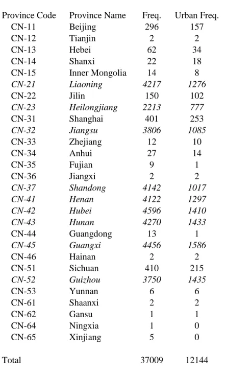
21 Table 1 (Appendix) shows the sample frequency by birth province. Most respondents were born in the
provinces sampled by the CHNS, which shows that province of birth and province of residence are highly correlated. Due to small sample size, I merge provinces based on geographic proximity.
22
famine, I use birth dates and province of birth to find the age (in months) of first exposure
and the duration (in months) of exposure to moderate, severe, and devastating famine.
Furthermore, I create age and duration categories for exposure to famine. Age
categories of first exposure consist of no exposure, exposure in utero, between birth and
age 1, between ages 1-3, and between ages 3-5. Duration categories of exposure consist of
no exposure, exposure to 1-3, 4-6, 7-12, 13-24, and 25+ months of famine. Creation of age
and duration categories aids interpretation of famine coefficients.232425 I assume that the
effects of famine differ depending on the stage in early childhood development of first
exposure; for instance, an individual who first experiences famine in utero is affected
differently than one who first experiences it at age five, all else equal.
4.3. Health Outcomes
Health outcomes of interest include original and residual height, original BMI, high
BMI, health index, incidence of serious illness, incidence of hypertension, and blood
pressure categories. Residual height is the deviations in height from the gender means.
High BMI indicates whether an individual’s BMI is in the upper 25% of the gender
distribution. Health index is the predicted health status based on an ordered Probit
regression of health status against incidence of hypertension, blood pressure categories,
weight, and other health measures. Incidence of serious illness (a binary variable) includes
23 If age (in months) is treated as a continuous variable, the resulting famine coefficient suggests that an
increase in age of first exposure from 0 to 1 month has the same effect on health outcomes as an increase in age of first exposure from 68 to 69 months of age. Hence, the creation of age categories is appropriate to aid interpretation.
24 Duration of exposure is measured as the total number of months in utero and early childhood that an
individual is exposed to famine. If an individual experience multiple instances of famine, “breaks” in exposure during that time period do not factor into the calculation of famine duration.
25 One issue with duration categories is that I assume continuous famine has the same effect on health
23
incidence of diabetes, infarction, and stroke. These health measures of interest are
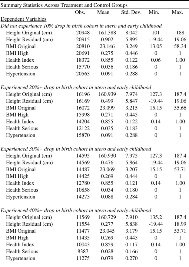
determined through data availability and sample size sufficiency. Table A1 in the Appendix
provides summary statistics for the dependent health variables across treatment and control
groups.
Table 2 (Appendix) provides summary statistics for the health variables across
treatment and control groups. Adult height appears to decrease with more severe exposure.
Similarly, BMI original is inversely related to famine severity, and individuals who were
exposed to famine have lower frequencies of high BMIs. Exposure to more severe grades
of famine also appears to be associated to lower frequencies of serious illness and
hypertension.
4.4. Other Variables
In my health equations, I also control for gender, age, age squared, ethnicity, urban
province of birth, level of schooling26, parents’ years of schooling27, and birth province and
survey year fixed effects. Parental education serves as a proxy for an individual’s
socioeconomic environment in early childhood and factors associated to parental
intra-household resource allocation behavior.
Table 2 provides summary statistics for the control variables. Ages range from 22
to 58 (an individual born in 1967 is 22 in 1989, the first round of the survey; an individual
born in 1953 is 58 in 2011, the latest round of the CHNS). The sample consists of more
females and rural residents.
26 Level of schooling is the highest level of schooling achieved and is broken down into none, primary, lower
middle, and upper middle and above.
24 5. Empirical Strategy
My empirical strategy exploits temporal, regional, and individual variation in
famine exposure. Since health outcomes are first observed in 1989, nearly thirty years after
the famine, my sample of interest includes individuals who were conceived or young
children during the time of the famine. I assume that exogenous shocks that occur during
this critical period have persistent effects on later-life outcomes.28 Furthermore, I assume
that exposure to famine at varying ages and lengths of time during the critical period is
likely to have different effects on health outcomes. My empirical strategy allows me to
measure the effects of in utero and early childhood famine exposure on later-life health
outcomes.
This section is organized as follows. Section 5.1 gives the empirical framework for
the baseline health equation, and Section 5.2 provides the results from the baseline analysis.
The revised baseline health equation with margins of famine intensity can be found in
Section 5.3. Section 5.4 provides the results for the effects of famine margins on health
outcomes.
5.1. Baseline Health Equation
I begin with my estimations with a baseline model for the effects of early life famine
exposure on later-life health outcomes. The basic health equation is given as:
𝐻𝑖𝑡𝑝𝑠 = 𝛾𝐹𝑖𝑡𝑝+ 𝛽𝑋𝑖𝑡𝑝+ 𝜑(𝐴𝑔𝑒𝑖𝑡𝑠) + 𝜋𝑃𝑡+ 𝛼𝑝+ 𝜇𝑠+ 𝜀𝑖𝑡𝑝𝑠, (5)
25
where
H
itpsis the health outcome for individual i born in time t in province p observed insurvey s. The famine “treatment” variable, denoted 𝐹𝑖𝑡𝑝, takes a value of 1 if an individual
is exposed to famine while in utero or in early childhood. 𝑋𝑖𝑡𝑝 denotes the vector of other
time-constant explanatory variables including gender, ethnicity, urban place of residence,
level of schooling, and parents’ years of schooling, and 𝜑(𝐴𝑔𝑒𝑖𝑡𝑠) is a quadratic
polynomial of age. I also include a dummy variable for post-famine years (which takes a
value of 1 if
t
>
1962
), birth province fixed effects, survey year fixed effects, and an errorterm, which are denoted 𝑃𝑡, 𝛼𝑝, 𝜇𝑠, and 𝜀𝑖𝑡𝑝𝑠, respectively. The effect of interest is 𝛾 and
represents the effect of the three different definitions of famine “treatments” on health
outcomes.29
In my empirical model, the vector of health outcomes includes original and residual
height, BMI, incidence of high BMI, health index, incidence of serious illness, and
incidence of hypertension. Depending on the nature of the health variable, I use OLS and
Probit regressions in my baseline estimation.
I use a straight-forward OLS regression to estimate the effects of famine exposure
on original and residual height, BMI, and health index. Occurrence of famine, age, age
squared, gender, ethnicity, and urban place of residence are all exogenous regressors in
Equation (5).303132 Furthermore, differences in birth provinces are controlled for by birth
29 As mentioned in Section 4, an individual is designated to have experienced moderate, severe, and
devastating famine if, between conception and age five, he or she experienced a drop in relative birth cohort of 20%+, 30%+, and 40%+ respectively.
30 Level of schooling and parents’ years of schooling are arguably exogenous. However, it may be argued
that exposure to famine in utero and early childhood affect later-life educational attainment.
31 A possible limitation is that relative birth cohort may measure famine with error. Since measurement error
is likely random, it may attenuate the OLS estimations (Meng and Qian, 2009).
32 As Chen and Zhou (2007) point out, fertility may be systematically correlated with individual
26
province fixed effects and individual effects in the CHNS are controlled for by survey year
fixed effects.33 Finally, I include a dummy variable for post-famine years, which takes a
value of one if an individual is born after 1962, that allows me to avoid collinearity between
age and survey year. Hence, OLS produces the most consistent and unbiased results for the
continuous health variables.
I use Probit regressions to estimate the effects of famine exposure on the binary
health variables, which take values of 0 or 1 depending on whether individuals experience
high BMIs, serious illnesses, and hypertension. This is the standard model for treating
binary response variables.
My baseline health equation assumes that exposure to famine in utero and early
childhood has persistent effects on later-life health outcomes. Furthermore, I hypothesize
that exposure to severe or devastating famine increases the likelihood for adverse health
characteristics later in life. As expounded in the theoretical section, exposure to more
severe grades of famine could affect health outcomes directly through causing larger
changes in the underlying production function and indirectly through parental behavior and
health investment decisions.
5.2. Baseline Health Estimates
In this section, I describe the results from the baseline health estimations. The
analysis compares the effects of different famine “treatments” on the health outcomes.
Table 3A (Appendix) gives the results for Original and Residual Height, Table 3B
(Appendix) gives the results for BMI and High BMI, and Table 3C (Appendix) gives the
33 For instance, regions with poor institutions may be more prone to famine. Additionally, using birth
27
results for Health Index, Health Serious, and Hypertension. In all tables, I include the
coefficients for all covariates in the baseline equation.
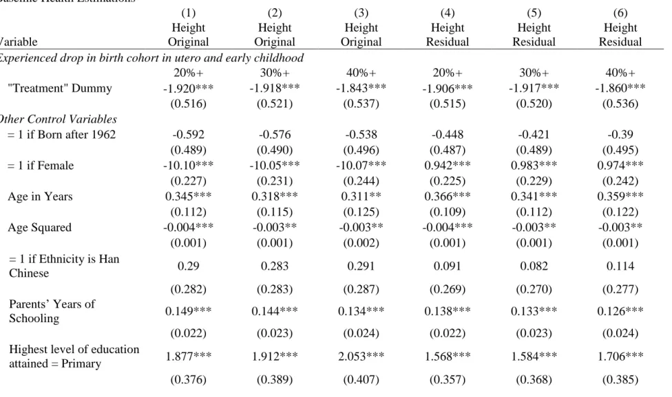
Table 3A gives the baseline estimates for height. According to Col. 1-3, exposure
to moderate, severe, and devastating famine is associated to decreases in height of 1.920,
1.918, and 1.843 cm respectively. All coefficients are highly significant at the 0.01 level.
These results are corroborated by the impact of exposure on residual height. Col. 4-6
indicate that exposure to moderate famine decreases residual height by 1.906 cm while
exposure to severe and devastating famine decreases residual height by 1.917 and 1.860
cm respectively. These height results suggest that exposure to famine adversely affects an
individual’s height, but the adverse effect on adult height decreases with more severe
famine.
Table 3B presents the baseline estimates for BMI. According to Col. 1-3, exposure
to moderate, severe, and devastating famine is associated to decreases in BMI of 0.987,
0.988, and 0.822 points respectively. All coefficients are highly significant at the 0.01 level.
Furthermore, I observe that individuals exposed to famine are less likely to have high
BMIs. Individuals exposed to 20%+, 30%+, and 40%+ drops in relative birth cohort in
utero and early childhood are 8.2%, 8.8%, and 5.6% less likely to be in the upper 25% BMI
of their gender distribution.
Tables 3A and 3B also give the coefficients for the control variables. Estimates for
parents’ level of schooling are positive and highly significant for original and residual
height. This matches expectations; I use parents’ years of schooling as a proxy for early
childhood socioeconomic environment, and more years of schooling suggest higher levels
28
height is positive and highly significant for all levels of schooling. Furthermore, I observe
that a higher level of education is associated with a larger increase in height, and this holds
true across all famine “treatments”. In contrast, the effect of an individual’s level of
schooling on BMI is insignificant unless the individual attains at least an upper middle
school education. Attaining an upper middle and above level of education also has a
positive and statistically significant effect on incidence of high BMI.
Table 3C gives the baseline estimates for health index, incidence of serious illness,
and incidence of hypertension. According to Col. 1-3, exposure to moderate, severe, and
devastating famine decreases the health index by 0.018, 0.017, and 0.013 points
respectively, and the first two estimates are statistically significant at the 0.05 level. Col.
4-6 show that exposure to moderate, severe, and devastating famine decreases the
incidence of serious illness by 4.5%, 4.4%, and 2.7% respectively, and these estimates are
statistically significant. Furthermore since the magnitudes are decreasing, it appears that
exposure to more severe grades of famine decreases the likelihood for a serious illness.
Col. 7 and 9 suggest that exposure to moderate and devastating famine decreases the
incidence of hypertension by 2.7% in both cases.
Similarly, I include the coefficients for my control variables. Effects of parents’
years of schooling on the health index and incidence of serious illness are positive and
statistically significant. Furthermore, compared to individuals with no formal education,
individuals who only attained a primary school level of education are more likely to get a
serious illness. It also seems females are less likely to get hypertension, particularly when
29
5.3. Baseline Health Equation with Margins of Famine Intensity
In order to create heterogeneity of treatment at the individual level, I interact famine
“treatment” with margins of famine intensity. This produces the second-stage health
equation:
𝐻𝑖𝑡𝑝𝑠 = 𝛾𝑀𝐹𝑖𝑡𝑝∙ 𝑀𝑖𝑡𝑝+ 𝛽𝑋𝑖𝑡𝑝+ 𝜑(𝐴𝑔𝑒𝑖𝑡𝑠) + 𝜋𝑃𝑡+ 𝛼𝑝+ 𝜇𝑠+ 𝜀𝑖𝑡𝑝𝑠, (6)
where 𝐹𝑖𝑡𝑝∙ 𝑀𝑖𝑡𝑝 represents the interaction term between famine “treatment” and margins
of famine intensity. Margins of famine intensity include age (months) of first exposure to
famine, age categories of first exposure, duration (months) of exposure, and duration
categories of exposure. Including these interaction terms allows me to create
individual-specific experiences of famine based on timing and place of birth and hence serves as a
more precise proxy for famine. Further, I am able to study the effects of timing and length
of exposure to moderate, severe, and devastating famine on adult health outcomes.
Similar to my baseline health model, I hypothesize that individuals who are
exposed at earlier ages to longer periods of famine are more likely to display adverse health
characteristics later in life. For the remainder of this paper, I only present health estimates
for the effects of “Severe” famine. However, I compare these estimates to those derived
under “Moderate” and “Devastating” famine to check for robustness.
5.4. Baseline Health Estimates with Margins of Famine Intensity
In this section, I summarize the results of the baseline health estimates with margins
of famine intensity. Table 4 (Appendix) gives the main results for age categories of first
exposure and duration categories of exposure to severe famine. Each regression includes
30
As seen in Section 5.2, exposure to severe famine has a negative effect on original
and residual heights. While all age categories of first exposure have negative coefficients,
exposure between birth and age one is statistically significant and highly negative. This
indicates that exposure to famine in the first year of life, which decreases original and
residual heights by 2.51 and 2.57 cm respectively, has a disproportionate effect on adult
height compared to other age categories. Exposure at later stages in early childhood appears
to have a decreasing effect on adult height though the results for later age categories
decrease in statistical significance. Furthermore, Col. 1 and 2 suggest that longer exposures
to famine generally have more negative effects on adult height. Exposure to 4-6, 13-24,
and 25+ months of famine decreases original height by 2.33, 2.48, and 2.61 cm
respectively.
Col. 3-4 show the effects of margins of famine intensity on BMI. Exposure in utero,
between ages 0 and 1, and between ages 1 and 3 decreases original BMI by 1.01, 0.67, and
0.63 points respectively, and all estimates are statistically significant. This suggests that
earlier exposure to famine has a larger negative effect on BMI. The results for duration
categories of first exposure suggest that any length of exposure adversely affects original
BMI. These results are corroborated by the results for incidence of high BMI. Col. 4 also
shows that earlier and shorter exposures decrease the likelihood for incidence of high BMI.
However, those exposed to famine are less likely to have high BMIs compared to those
unexposed.
In Col. 5, exposure to famine between ages 1-3 decreases the health index by 2.8%.
Additionally, exposure to > 2 years of severe famine decreases health status by 2.9%. Col.
31
illness while for duration categories between 1-24 months, longer periods of exposure
seems to decrease likelihood for serious illness. Finally Col. 7 shows that first exposure
between birth and age one decreases the incidence of hypertension by 2.9% while 4-24
months of exposure seem to decrease the incidence of hypertension by approximately 4%
compared to those who were not exposed.
Overall, the results for the baseline health estimations with margins of famine
intensity suggest that exposure to famine decreases adult height, BMI, health index, and
incidences of serious illnesses and hypertension. Furthermore, famine exposure between
ages 0 and 1 (and earlier exposure, in general), has the largest negative effect on adult
height while the later the exposure, the less famine affects BMI. Exposure at later ages in
the critical period has larger, more negative effects on the health status. Finally, adult height
generally decreases with increased length of exposure.
6. The Selective Mortality Issue
In the remainder of this paper, I address the selective mortality issue. As mentioned
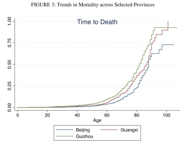
above, I believe selective mortality may bias my baseline health estimates. Figure 3
highlights the survival trends for Beijing, Guangxi, and Guizhou. I observe that at each age
past sixty, the frequency of mortality is highest in Guizhou, followed in decreasing order
by Guangxi and Beijing. In comparing these trends to EDR in 1960, the worst year of the
famine, I find a direct relationship between EDR and frequency of death.34 From a
descriptive point of view, it appears that individuals in provinces with more acute
experiences of famine are more likely to die at younger ages.
32
As with all panels, the CHNS is subject to attrition due to mortality. Furthermore,
mortality is non-random (since individuals with “poorer” health are more likely to die),
and I observe selection into survival. If this selective mechanism depends on unobserved
characteristics that also affect the outcome variables of interest, it could bias my estimates
(Gerry and Papadapoulos, 2013). In the context of my study, selection bias arises when
participants exhibit some characteristics that affects both the probability of participation in
future periods as well as the health outcome.
FIGURE 3: Trends in Mortality across Selected Provinces
33
Exposure to famine affects mortality during the time of the survey either directly
or indirectly through its effect on observed and unobserved health characteristics.
Characteristics that positively affect health also increase the likelihood for survival and
vice versa, confounding the relationship in the first-stage health equation. Hence, failing to
account for selective mortality bias may underestimate the effects of famine. In order to
correct for selective mortality bias in the baseline health equations, I use IPW and Joint
Modeling techniques.
6.1 Inverse Probability Weighting
IPW estimators enable researchers to account for selection on observables. (In the
case where unobserved factors affect both the selection process and the dependent
variables, in order to produce consistent estimates, we need to find at least one exclusion
restriction. This is difficult since the decision to participate in the survey (i.e. mortality) is
likely to affect health outcomes. Hence, we in this section we restrict ourselves to the case
where selection occurs on observable factors.35) We assume that observable factors affect
both the dependent outcome and selection into participation (i.e. survival).
The idea behind IPW is that conditional on observables, 𝑋𝑖𝑡𝑝, 𝐿𝑖𝑡𝑝(𝑠−1), selection
becomes random. Since respondents may become censored at any point after the first
period, the vector of time-varying observables contains information from the most recent
uncensored survey round. Furthermore, conditional on observables from the previous
period, the probability distribution for survival does not depend on either the unobserved
or observed covariates of any other period (Gerry and Papadaloupos, 2013).
35 See Gerry and Papadaloupos (2013) for a more detailed explanation of the constraints to the selection on
34
For my purposes, 𝑋𝑖𝑡𝑝, 𝐿𝑖𝑡𝑝(𝑠−1) includes blood pressure, gender, age, age squared,
ethnicity, urban, parents’ years of schooling, level of schooling, and birth province and
survey year fixed effects. The econometric procedure is as follows: I use a Probit model to
regress death against my vector of covariates and predict the likelihood of mortality 𝑝̂𝑖𝑡𝑝𝑠.
Then, I construct inverse probability weights such that the predicted probability of
participation in period s is:
𝑤̂𝑖𝑡𝑝𝑠 =𝑝̂1
𝑖𝑡𝑝𝑠. (7)
In the last step, I weight my baseline health function by 𝑤̂𝑖𝑡𝑝𝑠, according higher “weights”
to individuals who are more likely to die before the next survey round and thereby
correcting for selective mortality bias on observed factors.
6.2 Joint Modeling
However, longitudinal and survival processes are often related through unobserved
factors. For instance, it may be the case that another measure of health (unobserved in the
data) is strongly associated with likely death and that individuals with this unobserved
characteristic are also the least healthy in terms of observed health characteristics. In this
case, separate modeling results in biased estimates, and joint modeling is required to
control for unobserved factors. I am interested in examining the effects of famine
“treatment” on survival vis-à-vis a longitudinal process. If the joint modeling estimates
show that famine does have an effect on survival even after controlling for observed and
unobserved random effects, this is further evidence that selective mortality does bias the
35
I use the Joint Modeling of Longitudinal and Survival Data method proposed by
Crowther, Abrams, and Lambert (The Stata Journal) to estimate the effects of famine on
survival through the observed health covariates. The general framework is to assume a
mixed-effects model for the longitudinal data and an exponential model for the survival
data, and the two models share some random effects of variables (Wu et al., 2012). A
standard formulation is presented as such. For the longitudinal submodel:
ℎ𝑖𝑡𝑝𝑠 = 𝐻𝑖𝑡𝑝𝑠+ 𝜀𝑖𝑡𝑝𝑠, where 𝜀𝑖𝑡𝑝𝑠~𝑁(0, 𝜎𝜀2) (8)
𝐻𝑖𝑡𝑝𝑠 = 𝛾𝐹𝑖𝑡𝑝+ 𝛽𝑋𝑖𝑡𝑝+ 𝑏𝑖𝑍𝑖𝑡𝑝+ 𝜋𝑃𝑡+ 𝛼𝑝+ 𝜇𝑠, (9)
where the longitudinal responses, hitps, are measured with error, 𝑋𝑖𝑡𝑝 and 𝑍𝑖𝑡𝑝 are design
matrices for fixed (𝛽) and random (𝑏𝑖) effects respectively. I assume the measurement error
in a given period is independent of the random effects and of error in previous periods. The
health vector 𝐻𝑖𝑡𝑝𝑠 represents the vector of “true” health outcomes.
I assume an exponential distribution for my survival model. Hence, my survival
model is specified as such:
ℎ(𝑠|𝑏𝑖, 𝑣𝑖𝑡𝑝) = ℎ0(𝑠)exp(𝜌𝐻𝑖𝑡𝑝𝑠 + 𝛿𝑣𝑖𝑡𝑝), (10)
where ℎ0(𝑠) is the baseline hazard function, 𝑣𝑖𝑡𝑝denotes my set of covariates that serve as
predictors for survival, and 𝜌 is the association parameter between my longitudinal
response and survival. In this submodel, the value of the longitudinal response is included
as a time-varying covariate of survival. Fundamentally, Joint Modeling assumes there are
some random, unobserved processes underpinning both the longitudinal responses and
survival. From the theoretical discussion, I believe famine could cause unobserved shifts
36
and hence require joint modeling to trace the effect of famine on mortality through its effect
on the longitudinal response.
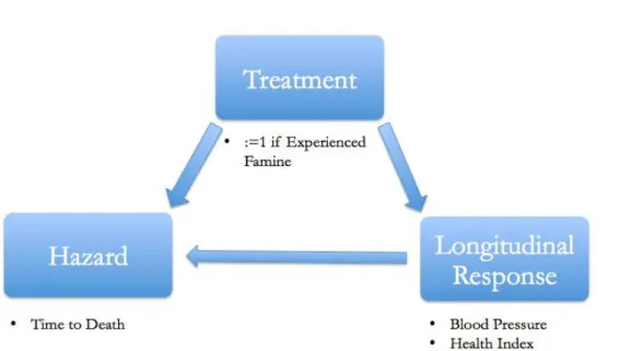
Figure 4 diagrams the effect of the famine “treatment” on mortality, both directly
and indirectly through its effect on a longitudinal marker in all previous periods. In the
context of my study, I use blood pressure and health status as my longitudinal response
variables.36 Blood pressure is normally distributed, but health status is left-skewed. Thus,
I use health status squared in the regression. Famine “treatment” is specified as exposure
in utero and early childhood to a 30%+ drop in relative birth cohort, and the hazard variable
is mortality. I also control for post-famine years, age, age squared, gender, ethnicity, and
years of schooling. I am hence measuring the effects of famine exposure on survival,
accounting for unobserved random effects that factor simultaneously in my survival and
longitudinal submodels.
37
By jointly modeling the longitudinal and survival processes, I obtain the overall
effects on survival through combining the direct effects on survival and the direct effects
on the longitudinal response, multiplied by an association parameter. Since famine could
impact survival through its effects on later-life health outcomes, jointly modeling serial
longitudinal values and survival may carry important insight into the underlying health
production technology.
7. Estimations Correcting for Selective Mortality Bias
In this section, I present the revised health estimates after accounting for selective
mortality bias. Section 7.1 gives the IPW results, Section 7.2 compares the results from the
weighted and unweighted estimations, Section 7.3 gives the results from the Joint
Modeling estimations, and Section 7.4 compares the IPW and Joint Modeling estimations. FIGURE 4: Joint Modeling Diagram
38 7.1. Inverse Probability Weighting Results
Following the econometric procedure, I reweight my original baseline health
equation with margins of famine intensity to account for selective mortality. Table 5
(Appendix) summarizes the main IPW results.37
Exposure to severe famine has a negative effect on original and residual heights.
While all age categories of first exposure have negative coefficients, exposure between
birth and age one is statistically significant and highly negative. This indicates that first
exposure to famine in the first year of life decreases original and residual heights by 2.04
and 2.10 cm respectively. Exposure at later stages in early childhood appears to have a
decreasing effect on adult height though the results for later age categories are significant.
Furthermore, Col. 1 and 2 show that 4-6 months of exposure to severe famine decreases
original and residual height by 1.78 and 1.75 cm respectively.
Col. 3 and 4 show the weighted estimates of famine on BMI measures. Exposure
to severe famine has a negative and statistically significant effect on both original BMI and
incidence of high BMI. Furthermore, exposure to severe famine in utero decreases BMI by
0.79 points and decreases the likelihood for high BMI by 11.7%. The effect of exposure
between ages 3-5 is also significant: these individuals are 14.2% less likely to have high
BMI compared to those who were never exposed to famine.
Col. 5 suggests that individuals first exposed to severe famine at later stages in early
childhood and for shorter durations have lower health indices. Col. 6 indicates that
individuals exposed to famine in the first year of life are 1.86% less likely to get a serious
illness while individuals exposed for 4-6 and 7-12 months are 4.24% and 4.18% less likely
37 Table 5A (Appendix) summarizes the IPW results for the baseline health equation and serves as a check
39
than individuals who did not experience famine. Finally Col. 7 shows that first exposure
between birth and age one decreases the incidence of hypertension by 3.75% while
exposure to 7-12 months of famine decreases the incidence by 2.93% compared to those
not exposed.
7.1. Comparing Weighted and Unweighted Estimations
Given my research interest in the effects of the Great Chinese Famine on later-life
health outcomes, factors that proxy “health” such as blood pressure and years of schooling
are likely related to mortality and the health variables of interest. If the two stages result in
very different sets of estimates, a non-random selective mechanism could bias my baseline
health estimates.
Since the IPW estimation method predicts an individual’s probability of survival
conditional on observed factors such as blood pressure, gender, and ethnicity and then
reweights the sample to ensure representativeness following selective mortality, the IPW
estimates produce less biased health results. However, in order to discuss deviations
between the unweighted and weighted estimates, I perform significance tests to check and
confirm that these estimates are statistically different.38
In comparing the weighted and unweighted estimates, the effect of exposure to
severe famine on height loses its statistical significance. Exposure to famine in the first
year of life remains negative and statistically significant, though the magnitude of decrease
is smaller in the weighted case. Finally, while the unweighted estimates suggest an inverse
38 Results from the t-tests suggest that I can reject the null hypothesis that the means of the weighted and
40
relationship between duration of exposure and adult height, this relationship does not
appear in the IPW estimates.
The IPW estimates for BMI preserve the general trend that individuals who
experienced earlier and shorter periods of famine are most likely to have lower BMIs.
However, individuals exposed between ages 3-5 are 14.2% less likely to have high BMIs
in the weighted analysis compared to 6.9% (statistically insignificant) less likely in the
unweighted analysis.
Using IPWs, estimations for the effects of famine on health index are significant.
To a greater extent than in the unweighted analysis, there is a clear inverse relationship
between age of first exposure and health index; the older the stage of first exposure, the
larger decrease on the health index. Furthermore in the weighted analysis, shorter periods
of exposure do appear to have negative effects on health status compared to longer periods
of exposure and no exposure.
Similar to Col. 6 of Table 4, Col. 6 in Table 5 indicates that exposed individuals
are less likely to get a serious illness, and the magnitude of the effects are roughly the same.
Finally, individuals exposed to famine in the first year of life are less likely to get
hypertension in the weighted analysis. When comparing duration categories, I find that
individuals exposed to 7-12 months of severe famine are more likely to get hypertension
in the weighted analysis compared to the same exposed individuals when failing to account
for selective mortality bias.
While weighted estimates still show a negative effect of famine on adult height, it
is surprising that the magnitudes of these effects are smaller than in the weighted
41
CHNS or displayed characteristics of likely death are on average taller than the estimated
average in the baseline health equation. For BMI, earlier and shorter exposures to severe
famine decrease BMI. These magnitudes are larger in the weighted estimations, indicating
that individuals who were exposed to famine for 1-3 and 4-6 months and are likely to
become censored due to selective mortality also displayed lower BMIs on average.
Furthermore using IPWs, exposure to famine has a statistically significant and
negative effect on health status. This indicates that individuals who were exposed to famine
and displayed characteristics of likely death also reported lower health statuses. It is
interesting to note that exposure at later age categories decreases the health index; a
possible explanation is that earlier exposure to famine allows more time in the critical
period to invest in health and counter famine’s early effects. Hence, exposure to famine
may have more of an effect on health index through the behavioral effect. Unlike height or
weight, health status is a subjective health measure and may therefore be less influenced
by the underlying health production function than objective health measures. A further
explanation may be that individuals who experienced famine at later stages in the critical
period are more likely to remember undergoing the famine, which could lower their
perceived health status.
Finally, exposure to severe famine decreases the likelihood for serious illness.
Recall, serious illness includes diabetes, stroke, and infarction. In all three of these
illnesses, obesity is a serious risk factor.39 However, since exposure to famine decreases
BMI, it makes sense that individuals who were exposed to famine are also less likely to get
39 “Obesity increases coronary artery disease, myocardial infarction, and stroke risk. Obesity increases strain