GRAPHICAL MODELS FOR HIGH DIMENSIONAL DATA WITH GENOMIC APPLICATIONS
Jenny Yang
A dissertation submitted to the faculty of the University of North Carolina at Chapel Hill in partial fulfillment of the requirements for the degree of Doctor of Philosophy in
the Department of Biostatistics in the Gillings School of Global Public Health.
Chapel Hill 2017
Approved by:
Wei Sun
c ○ 2017 Jenny Yang
ABSTRACT
Jenny Yang: Graphical Models for High Dimensional Data with Genomic Applications (Under the direction of Wei Sun)
Many previous studies have demonstrated that gene expression or other types of -omic features collected from patients can help disease diagnosis or treatment selection. For example, a few recent studies demonstrated that gene expression data collected from cancer cell lines are highly informative to predict cancer drug sensitivity (Garnett et al. 2012, Barretina et al. 2012, Chen et al. 2016b). This is partly because many cancer drugs are targeted drugs that perturb a particular mutated gene or protein, and thus having that mutation, or observing the consequence of such mutation in gene expression data, is highly informative for drug sensitivity prediction. Such systematic studies of drug sensitivities require giving different drugs in a series of doses to the same cell line, which is obviously not possible for the human studies. More sophisticated methods are needed to estimate potential effects of cancer drugs based on observational data. Since the effect of a targeted cancer drug can be considered as an intervention to the molecular system of cancer cells, a directed graphical model for gene-gene associations is a natural choice to model the molecular system and to study the consequence of such interventions.
ACKNOWLEDGMENTS
After a good three and a half years of this labor of love, the inumerable times when I thought this would never be complete, it is finally time for me to look back on my journey and recognize everyone who has held me up on their shoulders to get me here. First, a special thanks and deep gratitude to my advisor, Dr. Wei Sun. He was rare in his support of me and my work, in his patience for my struggles, and in his generosity with his time and funding. I would also like to thank my committee for their patience and insight into my work. Especially, Drs. Donglin Zeng and Stephanie Engel who were instrumental in guiding my transition from coursework to dissertation.
Secondly, I’d like give a shout-out to UNC’s ITS computing. In my entire time at UNC, they haven’t let me down once with prompt replies to my panicked emails.
Finally, I would like to thank my invaluable support network. My friends that kept me sane by commiserating and supporting me. Who believed in me, although all evidence might be pointing to the contrary. Especially Briana Stephenson and Emily Butler, who My parents, who sacrificed their entire way of life to bring me to the U.S. and keep me here. My father, who always emphasized the importance of academics and was my role model in obtaining a PhD. My mother, who inspires me everyday with her work ethic. My brothers for always being there with an encouraging word. Especially Philip, who never hesitated to travel back home when I needed him to take care of something because I needed to work or travel.
TABLE OF CONTENTS
LIST OF TABLES · · · xi
LIST OF FIGURES · · · xii
CHAPTER 1: LITERATURE REVIEW · · · 1
1.1 Graphical Models . . . 1
1.1.1 Undirected Graphical Model Estimation . . . 2
1.1.2 Directed Acyclic Model Estimation . . . 4
1.1.3 Considering Model-Free Settings . . . 7
1.2 Single-Cell RNA-Seq Data . . . 9
1.2.1 Data Generation . . . 10
1.2.2 Statistical Analysis Challenges . . . 11
1.2.3 Current Approaches for Analyses . . . 12
1.2.4 Summary . . . 15
CHAPTER 2: MODEL-FREE ESTIMATION · · · 16
2.1 Algorithm . . . 16
2.1.1 Step 1: Estimation of the Moral Graph . . . 16
2.1.2 Step 2: Estimation of the Skeleton . . . 18
2.2 Theoretical Properties . . . 22
2.3 Implementation Considerations . . . 25
2.3.1 mGAP . . . 25
2.4 Simulation . . . 27
2.5 Application to TCGA Data . . . 31
2.5.1 Data Source . . . 31
2.5.2 Analysis Results . . . 32
2.6 Discussion . . . 38
CHAPTER 3: GRAPHICAL MODEL FOR SCRNA-SEQ DATA · · · 41
3.1 Overall Algorithm . . . 41
3.1.1 Step 1: Neighborhood selection . . . 43
3.1.2 Step 2: Testing Conditional Independence . . . 48
3.2 Implementation Details . . . 48
3.3 Simulation . . . 50
3.3.1 Set-up . . . 50
3.3.2 Results . . . 51
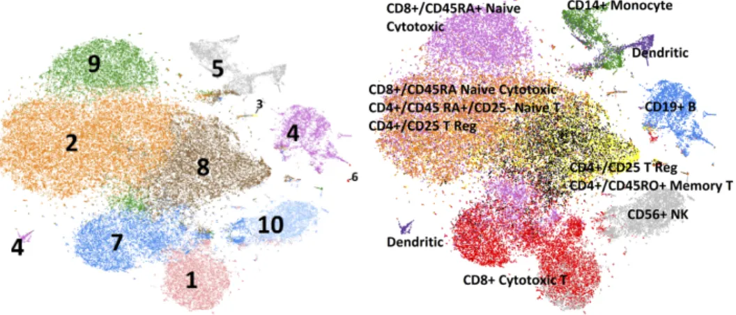
3.4 Application to Peripheral Blood Mononuclear Cell Data . . . 52
3.4.1 Data Sourcing and Processing . . . 52
3.4.2 Clustering . . . 52
3.4.3 Results . . . 55
3.5 Discussion . . . 56
CHAPTER 4: CONCLUSION · · · 62
APPENDIX A: ALGORITHMS FOR MODEL-FREE APPROACH · · · 63
APPENDIX B: PROOFS FOR THEORETICAL RESULTS OF MGAP · · · · 64
B.1 Weak Oracle Property for Model Free Variable Selection . . . 64
B.1.1 Consistency of modified-PC Algorithm . . . 74
APPENDIX C: DERIVATION OF PENALTY WEIGHTS FOR SCZINB · · · · 78
C.2 When yi >0 . . . 80
APPENDIX D: DERIVATION FOR SCZINB APPROXIMATION · · · 82
APPENDIX E: PSEUDOCODE FOR SCZINB · · · 84
APPENDIX F: ADDITIONAL FIGURES AND TABLES · · · 87
LIST OF TABLES
2.1 Simulation Results using (2.4) with Effect Size 1 . . . 28
2.2 Simulation Results using (2.5) with Effect Size 1 . . . 29
2.3 Simulation Results using (2.4) and Effect Size 0.5 . . . 30
2.4 Simulation Results using (2.5) and Effect Size 0.5 . . . 31
2.5 Results for TCGA Breast Cancer Data . . . 32
2.6 Mean Results for Mardia’s Test of Multivariate Normality for Residuals of Exclusive Pairs . . . 34
2.7 Similarity and Differences between Estimates from Original and Cross-Validated Sample . . . 35
2.8 Dimension Reduction for Model-Free GG Simu-lation Results using (2.4) . . . 39
3.1 Full Simulation Results . . . 60
3.2 Log Penalty versus Lasso Penalty Simulation Results . . . 61
3.3 Subpopulation counts for full cell population and myeloid subpopulation. . . 61
LIST OF FIGURES
2.1 Estimated Graphs for TCGA Breast Cancer Data. . . 33 3.1 K-means clustering results compared with
clas-sification using subpopulation correlations for full
population. . . 54 3.2 K-means clustering results compared with
clas-sification using subpopulation correlations for Myeloid
Cells (Cluster 5). . . 54 3.3 Gene expression heatmaps for macrophages. . . 54 3.4 Full estimated graph of dendritic myeloid cells. . . 57 3.5 Full estimated graph of CD16-/low monocyte
myeloid cells. . . 58 F1 Comparison of coefficient sizes for pairs
exclu-sively selected by either PenPC or Model Free. . . 88 F2 Comparison of−log10(P-Values)Found by Monte
Carlo Simulation vs Imhof’s Exact Method across
CHAPTER 1: LITERATURE REVIEW
1.1 Graphical Models
Directed acyclic graphs (DAGs) are directed graphical models describing the con-ditional independence amongst a number of random variables [Pearl (2009)]. The “acyclic” part of the name refers to the constraint that there is no directed cycle (or loop) in the graph. This constraint is necessary for causal inference [Pearl (2009), Spirtes et al. (2000)]. Consider a set of p random variables, X := {X1, ..., Xp} with
true DAG structure ofG(0) := (V,E(0))– whereV :={X
1, ..., Xp}is the set of vertices
corresponding to X and E(0) is the set of directed edges. The skeleton of a DAG is defined as an undirected graph, obtained by removing the directions of all the edges in a DAG. A v-structure is a structure of X1 → X2 ← X3, where X1 and X3 are not directly connected. The DAGs that share the same skeleton and the same set of v-structures form a Markov equivalence class, and all the DAGs within the same Markov Equivalence class encode the same set of conditional independence relations of the p random variables.
For the purposes of this proposal, we focus on the problem of estimating a DAG from high dimensional observational data. Without randomized interventions, a popular assumption used in graphical model estimation is that of ordering. This is where we assume that for vertices X1, ..., Xp, a vertex with a smaller subscript will always be
most likely Markov Equivalence class.
Without knowing edge directions it is impossible to separate the parents of a node from its children, making estimation based on independence tests conditional on Xipa impossible. An alternative is to define the edge between Xi and Xj by Ei,j =I{Xi ⊥
Xj|X−(i,j)}, which allows us to do conditional independence testing based on observa-tional data. Following this edge definition, we can recover the moral graph, which is constructed by connecting the co-parents of v-structures of a DAG skeleton. Then, one way to estimate the skeleton of a DAG is to use a two-step process; first, estimating the moral graph, then removing the connection between co-parents of v-structures. In addition, even with observational data, we can orient a limited number of edges in the skeleton corresponding to v-structures. Such a partially directed graph can be used to make useful causal inference [Maathuis et al. (2009)]. This is the basic procedure we will propose.
1.1.1 Undirected Graphical Model Estimation
The most intensely studied area for estimating these moral graphs are concentrated on Gaussian Graphical Models (GGM) or the extended family of nonparanormal mod-els as dubbed by [Liu et al. (2009)].
Gaussian Graphical Models
GGMâĂŹs are graphical models with the underlying assumption that X ∼ Np(µ,Σ).
The edge set, E(0), is usually estimated by the non-zero entries of the precision matrix
Σ−1 where E
i,j =I(Σ−i,j1 6= 0).
introduced a method to produce and utilize simultaneous p-values corresponding to partial correlations allowing for model selection in a single step, which they improved upon a few years later [Drton and Perlman (2007)]. For p n problems, machine learning techniques such as penalized regression or penalized maximum likelihood esti-mate have be utilized. For example, [Meinshausen and BÃijhlmann (2006)] proposed the neighborhood selection approach, where the neighborhood of each node is estimated using penalized regression with theL1 penalty. Combining the results of neighborhood selection of all the p nodes provided the structure of the GGM. While this neighbor-hood selection method gives consistent estimates of sparse high dimensional graphical models, its estimation of precision matrix is not consistent. Several penalized likelihood algorithms have been developed to directly estimate the precision matrix by placing an L1 penalty on the off-diagonal entries of the precision matrix [Yuan and Lin (2006), Friedman et al. (2008)]. These penalized estimation methods use some tuning param-eters to tune the strength of the penalty. The optimal tuning paramparam-eters are often selected by scoring a series of models estimated from a pre-defined tuning parameter grid. For example, BIC was often used as the scoring function [Lam and Fan (2009)].
1.1.2 Directed Acyclic Model Estimation
There are two basic approaches that have been developed for estimating DAGs or DAG skeletons: search-and-score based algorithms and conditional independence test-ing algorithms. Search-and-score based algorithms generate scores (i.e. AIC, BIC,
log likelihood, Bayesian Dirichlet probability or Kullback-Leibler divergence) for DAGs and selects the one with the best score [Chickering (2003), De Campos and Ji (2011)]. This approach is computationally infeasible for high dimension problems with p n, where p is the number of variables and n is sample size. In contrast, the conditional independence testing algorithm is computationally much more efficient and can give consistent estimate of DAG skeletons in high dimensional settings [Ha et al. (2016a)]. Thus, for the purpose of this paper we chose to focus on conditional independence testing algorithms. First, we introduce some definitions.
Definition 1 from [Pearl (2009)] (d-separation)
A path pis said to be d-separated (or blocked) by a set of nodes Z if and only if:
(1) pcontains a chain i→m→j or a forki←m→j such that the middle nodem is in Z, or
(2) pcontains an inverted fork (or collider)i→m←j such that the middle node m is not in Z and such that no descendant of m is in Z.
A set Z is said to be d-separate X from Y if and only if Z blocks every path from a node inX to a node in Y.
Definition 2 from [Spirtes et al. (2000)] (Markov)
The distribution of V is Markov to G := (V,E) if and only if each variable Xj ∈ V,
(parents).
Definition 3 from [Spirtes et al. (2000), Kalisch and BÃijhlmann (2007)] (Faithfulness) A probability distribution P on Rp is said to be faithful with respect to a graph
G if conditional dependencies of the distribution can be inferred from so-called d -separation in the graph G and vice versa. More precisely: consider prandom variables
X={X1, ..., Xp} ∼P. Faithfulness ofPwith respect toGmeans: for anyi, j ∈Vwith
i6=j and any sets⊆V,Xi andXj are conditionally independent given{Xr;r∈s} ⇔
vertex i and vertex j are d-separated by the set s.
Faithfulness was originally defined by [Spirtes et al. (2000)] as when the only condi-tional independencies inP are those found by the Markov condition onG. It is apparent
then that the assumption of faithfulness is required to be able to use conditional inde-pendence testing graph estimation. This body of work is largely built on the following central theorem:
The PC-Algorithm and its Relatives
The PC algorithm was named after the first names of its two authors (Peter Spirtes and Clark Glymour). It assesses the existence of each edge in a graphical model by conditional independence testing. The following theorem provides some theoretical jus-tification for such testing.
Theorem 1 from [Spirtes et al. (2000)]IfPis faithful to some directed acyclic
graph, thenP is faithful to G if and only if:
(2) For all vertices X, Y, andZ such that X is adjacent toY and Y is adjacent to Z and X and Z are not adjacent, X →Y ←Z is a subgraph of G if and only if X and Z are dependent conditional on every set containing Y but not X or Z.
SGS algorithm is an early conditional independence testing algorithm for graphical model estimation [Spirtes et al. (2000)]. It is essentially a brute force method that starts with a fully linked undirected graph and then seeks to remove edges by evaluating all possible conditional independence tests. The application of SGS algorithm is limited by its high computational cost. The PC algorithm seeks to improve upon the SGS by testing as few d-separation relationships as possible. It takes the same fully linked
undirected graph input and then thins the edges by first using marginal independence testing, then conditional testing based on subsets of adjacent variables of size one, size two, and so on.
Extensive work has been done to improve upon the various limitations of the PC algorithm including its order dependency (PC-stable [Colombo and Maathuis (2014)]) and error accumulation from “unfaithfulness” (Conservative-PC [Lemeire et al. (2010)]), as well as to extend its statistical properties to non-paranormal graphical models [Har-ris and Drton (2013)]. While the PC algorithm and its derivatives have worst case computation time bounded by O(pd), their expected computation time is of the order
O(n2 ¯p d
), where d is the degree of vertices in the true DAG and ¯pd is the average of
p d
over all vertices.
to obtain a more accurate estimate of moral graph. Then the edges within the moral graph is further thinned by a modified PC algorithm, which searches across candidate
d-separation sets based on the original input moral graph. PenPC has better
perfor-mance than the PC algorithm and is computationally more efficient in high dimensional settings. All of these existing methods rely on the assumption that the data follow mul-tivariate Gaussian distribution or the data can be transformed to follow mulmul-tivariate Gaussian distribution for conditional independence testing. Furthermore, the penalized estimation of moral graph requires the assumption that one variable is associated with other variables through a linear regression model. In this dissertation, we proposed a new method that does not require these potentially restrictive assumptions.
1.1.3 Considering Model-Free Settings
Without the assumption that the data arises from either a multivariate normal dis-tribution or a multivariate Gaussian copula, constructing a graphical model becomes much more complicated. This is because multivariate normality provides a very conve-nient property which allows graphical structure to commute under convolution. Under the model-free setting we do not place distributional assumptions (e.g. Gaussian) or relationship assumptions (e.g. homoscedastic linearity) on the data. Therefore, the covariance of the data usually does not provide the graphical structure [Loh and Wain-wright (2013)]. Instead, we consider that under the assumption of a positive and continuous density for y, the local Markov property infers global and pairwise Markov properties. Hence, we use node-wise conditional independence inference with neigh-borhood selection in order to obtain the global Markov random field. Once we obtain the global Markov random field, it becomes a question of removing v-structures using conditional independence testing in order to obtain the final undirected skeleton.
space is a particularly challenging problem in the model-free setting. We examined the body of available methods which fall into the following categories: i) distance based with explicit estimation of conditional densities [Su and White (2007)], ii) discretizing the conditioning set and performing the independence testing within each bin [Huang (2010)], iii) testing for independence against some set of transformed conditioning space [Song et al. (2009)], and iv) tests which examine the embeddings of probability distri-butions into reproducing kernel Hilbert spaces (RKHS) [Zhang et al. (2012)].
Tests of type i) are difficult to utilize over a wide variety of conditioning spaces as explicit estimation of the conditional densities becomes very complex, especially as the conditioning space increases. For example, [Su and White (2007)] proposes a test which measures the distance between the conditional characteristic functions and requires explicit estimation involving multiple applications of the Nadaraya-Watson leave-one-out kernel regression technique. Tests of type ii) cannot be used effectively in cases of low sample size as discretizing the conditioning space means even lower sample size for each unconditioned test per bin. Tests of type iii) are actually weaker than testing strictly for nonparametric conditional independence. For example, [Song et al. (2009)] proposes a method which tests for whether there exists some function h and parameterθ0 such that the variables are independent given a single index function λθ0(Z) = h(Z
>θ
0) of Z. This is a weaker condition than conditional independence. For example, if X and Y depend on two different subsets of Z which have overlap, then even for X ⊥ Y|Z we cannot find a λθ0(Z) for which X and Y are conditionally
independent.
the RKHS from [Fukumizu et al. (2004)]. For some random vector (X, Y) on do-main X × Y, let HX and HY be the RKHS on X and Y, with kernel functions kX and kY, respectively. The cross-covariance operator from HX to HY is defined by the relation: hg,P
Y Xfi = EXY[f(X)g(Y)]−EX[f(X)]EY[g(Y)] for all f ∈ HX and
g ∈ HY. The conditional cross covariance operator of(X, Y)givenZ is then defined as ΣY X|Z = ΣY X−ΣY ZΣ−ZZ1ΣZX. We can view this conditional cross covariance operator
as the partial covariance between any two functions belonging toHX andHY given any function belonging to HZ. [Fukumizu et al. (2004)] shows that this cross-covariance
operator is related to the conditional independence if characteristic kernels are used, based on the following lemma:
Lemma 1 from [Fukumizu et al. (2007)] Denote X¨ ≡ (X, Z), k¨
X ≡ kXkZ, and HX¨ the RKHS corresponding to kX¨. Let the space of square integrable functions of X be denoted L2
X, and similarly define L2Y and
L2
Z. Assume HX ⊂ L2X, HY ⊂ L2Y, HZ ⊂ L2Z and that kX¨kY¨ is a characteristic kernel on (X × Y)× Z. The characteristic kernel ensures that the statistical features of the
data distribution are preserved by the kernel embedding in the RKHS space. Further, assume thatHZ+R is dense in L2(PZ). Then
ΣXY¨ |Z = 0 ⇔X⊥Y|Z (1.1)
1.2 Single-Cell RNA-Seq Data
degree of inter-patient heterogeneity, both in terms of molecular features (e.g., somatic mutations, gene expression) and a patient’s response to treatments [Garnett et al. (2012), Barretina et al. (2012)]. Even within the tumor tissue of one patient, the tu-mor cells may have different somatic mutations, which is referred to as intra-tutu-mor heterogeneity [Yap et al. (2012), Patel et al. (2014)].
RNA sequencing has traditionally been done on bulk tissue samples and thus a large number of cells at once (bulk RNA-seq). Analyses of this data would operate on the measure of mean values of signals from individual cells, overlooking internal interactions and heterogeneity within the cell population [Kolodziejczyk et al. (2015)]. However, advances in Next Generation Sequencing (NGS) now allow deep sequencing of a single cell. This paves the way to a variety of applications including understanding why some cells may be drug responsive but others are not and determining molecular states which may be specific to a disease for drug targeting; as well as new research techniques, such as cell level perturbations to dynamically probe cell function [Eberwine et al. (2014)]. Obtaining estimates for homogeneous subclusters of cells within a cancer promise a path towards precision medicine: medical practice tailored to the unique profile of a patient’s cancer. Graphical models, such as the directed acyclic graph (DAG), are among the most promising solutions.
1.2.1 Data Generation
transcription. Finally, the cDNA needs to be amplified for sequencing using PCR [Tang et al. (2009), Stegle et al. (2015)]. Sequencing itself is done by applying NGS, such as the Illumina sequencing solutions.
After obtaining the raw sequence data, bulk RNA-seq techniques can be applied for sequence alignment in order to summarize the sequences and finally obtain the total read counts (TReC) of each mRNA sequence [Love et al. (2015), Chen et al. (2016b)]. Due to the small amount of starting material, a large amount of amplification needs to be done. Since amplification efficiency can vary between cells simply due to technical variability, it is recommended to use extrinsic spike-ins or unique molecular identifiers (UMIs) to facilitate normalization across cells [Stegle et al. (2015)]. Extrinsic spike-ins are tagged RNA mixes with known sequences and quantities which are added to the cell prior to amplification, in order to produce normalization factors to adjust for amplification bias. Alternatively, UMIs operate like barcodes and allow read counts enumeration that are independent of amplification bias. In the ideal setting, full cover-age UMIs would provide data most free of technical variability, however there are many non-UMI-based protocols currently utilized.
1.2.2 Statistical Analysis Challenges
is essentially zero and the empirical distribution of data is different from what would be expected from censoring. Instead, the current suspected culprit for zero-inflation ranges from a variety of sources including drop out from amplification, inherent heterogeneity of cell expression, and technical factors [Kolodziejczyk et al. (2015), McDavid et al. (2016)]. Heterogeneity of cell size means that some cells may just have a larger amount of total nucleic acids. This is often normalized for using the ratio of RNA reads to spike-ins reads, termed the endogenous RNA size factor. A more general technique uses relative expression counts instead of raw counts [Stegle et al. (2015)].
The heterogneity between individual cells is not confined to gene expression, but also to cell health and function. The individual cells may be in varying states of degradation or even apoptosis. In order to control for these confounding factors, bulk RNA-seq quality control tools are often used to check the proportion of reads which map back to the genome, the proportion of reads of RNA versus spike-ins, and the use of PCA to cluster good quality cells from bad quality cells [Stegle et al. (2015)].
There are additional challenges more specific to graphical model estimation using scRNA-seq data. It has been shown that the robustness of networks derived from scRNA-seq data may be dependent upon composition of cell types [Mahata et al. (2014)]. scRNA-seq data also may reveal less meaningful associations between genes. For example, if two cells are in different phases of cell cycle, a large number of genes may be associated due to the cell-cycle effect. Therefore it is crucial to remove the effects of such confounding factors.
1.2.3 Current Approaches for Analyses
Clustering techniques used for bulk RNA-seq data, which were used to classify tis-sues into separate types, can be applied to scRNA-seq data. These techniques fall under either dimension reduction or hierarchical clustering techniques. They characterize a sample by its composition of cell types, defined by the expression profile of each cell cluster. Often, this is done in order to find a set of marker genes for easier identi-fication of these clusters in future samples. The identiidenti-fication of these marker genes are the subject of much study, and are usually found by either comparing differential expression of genes between clusters or identifying highly variable genes (HVGs). For scRNA-seq data, these techniques typically use either the Poisson or Negative Binomial distributions in order to model the TReC, which allows confounding covariates to be adjusted for and even account for spatial correlations using the well solved general-ized linear model solutions [Anders and Huber (2010), Hardcastle and Kelly (2010), Robinson et al. (2010)]. However, in the context of scRNA-seq data, it is difficult to tease apart true differing clusters or variability due to confounding factors such as cell cycle. Further, the idea of cell type within the same tissue is currently a poorly defined biological concept, and it is unknown whether transcriptional differences represent true subpopulations [Patel et al. (2014)].
algorithm has been incorporated into the estimation to reduce computation time [Yang et al. (2011)]. For even faster computation, the graphical lasso, a penalized Gaussian covariance estimation method has been developed and used in a large number of network reconstructions [Friedman et al. (2008)]. Within the context of scRNA-seq data, we can take advantage of the variability of gene expression between cells as a natural perturbation to infer gene-regulatory networks [Padovan-Merhar and Raj (2013), Segal et al. (2003), PeâĂŹer et al. (2001)].
Currently, the only graphical model proposed specifically for scRNA-seq data has come from [McDavid et al. (2016)]. They propose a penalized multivariate Hurdle model based on the exponential family for neighborhood selection. Consider variable y with its element-wise non-zero indicator variable vy. To fit this data into the multivariate
Hurdle model framework, they let f(y) have Normal density of mean ξ and precision τ2. Then, they excise zero from the support of f(y) and give it a density of f
0(y) = exp{vy[1/2 log(τ2/(2π)) + log(p/(1−p))−ξ2τ2/2] +yξτ2−y2τ2/2 + log(1−p)}. This
allows the full support ofy to be modeled under the exponential family while modeling the extraeneous zero expression. They simplify the form of the multivariate Hurdle model and give the following likelihood:
logf(y;θ) = vy>Gvy+vy>Hy− 1 2y
>
Ky−C(G,H,K) (1.2) where G,H and K are interaction parameter matrices and C(G,H,K) is a constant. Then each part of the likelihood pertains to the modeling of a specific contribution, where G parameterizes the interaction of the binary process, K parameterizes the
interaction of the continuous process, and H parameterizes the interaction between
binary and continuous process.
For variable selection, they impose anL1group penalty of the formλPa
p
θ>
aHaaθa
Typically this type of group penalty has been seen with Haa = I. However, this type
of group penalty, which causes all parameters in θa to vanish simultaneously, assumes
similar effect size and scale-equivariance across the parameters. This is distinctly not true in this case due to the different underlying model distributions for the indicator variable vy (binomial) and continuous variable y (Gaussian). The typical solution of scaling the design matrix is not an option in this case due to the different distribution assumption. Hence, the authors propose rescaling the estimated coefficients within the penalty with the Fisher information under the null model of θa = 0 as Haa and
show that it is equivalent to a score test of the null hypothesis that θ = 0 versus the alternative of θ6= 0.
1.2.4 Summary
CHAPTER 2: MODEL-FREE ESTIMATION
Recall that we denote a DAG skeleton by G= (V,E), where V ={X1, ..., Xp} and
E are the vertex set and the edge set, respectively. A moral graphGM= (V,EM) can be derived from a skeleton G by connecting the co-parents in all the v-structures in G. Our goal is to develop a model free and nonparametric method to estimate DAG
skeleton by a two step process. First, we estimate the moral graph using a penalized model-free regression. Then, we further thin the edges of the estimated DAG skeleton by removing false connections due to v-structures using the modified PC-algorithm with nonparametric conditional independence testing. The overall structure of the algorithm is presented below.
2.1 Algorithm
2.1.1 Step 1: Estimation of the Moral Graph
We employ a neighborhood selection approach to estimate the moral graph by es-timating the neighbors of each vertex in the moral graph separately, and then consol-idating the results. That is, we establish an edge Xi−Xj if either Xj is selected as a
neighbor ofXi orXi is selected as a neighbor ofXj. All the neighbors of a vertexXk in
the moral graph form its Markov Blanket. For neighborhood selection ofXk, we adopt
a model free variable selection method (multivariate group-wise adaptive penalization ormGAP) forXk against all the other variables, denoted byX−k [Sun and Li (2012)].
Sliced Inverse Regression (SIR) [Li (1991)]. Then, it performs variable selection and parameter estimation by minimizing a weighted multivariate L2 loss function with an adaptive group lasso penalty. Specifically, for response vertex Xk, it uses the following
objective function for some transformation functionr(·) with h-dimension output:
argminB,κ,ω
( h X
s=1
kr(Xk)s−X−kBsk2
ωs
+λ
p
X
j=1
kbjk+τ
κj
+λ
p
X
j=1
log(κj) +n h
X
s=1
log(ωs)
)
,
(2.1) where r(·)s is the sth dimension of r(·), Bs is the s-th column of coefficient matrix
B, which includes the p−1 regression coefficients for the regression with r(Xk)s as
response variable, λ and τ are tuning parameters, and kbjk =
q
Σh
s=1Bj,s2 is the L2 norm for the h coefficients of the j-th covariate. ωs’s and κj’s are the weights for the
objective function and the penalty term, and the last two terms in equation (2.1) add constraints on the sizes of ωs’s and κj’s. Then, the set of vertices associated with Xk
are {Xj ; kbˆjk>0}. Estimation is done using a coordinate descent algorithm.
The pseudo-code of the algorithm for estimating the moral graph is then: Algorithm 1: Moral Graph Estimation
Data: X
Result: GM = (V,E) for j = 1 to pdo
Lety =Xk and X=X−k.
Scale y and X to standard deviation of 1 and center to 0. yt←r(y).
Obtain tuning parameter grid λ, τ from Algorithm 4 in Appendix A.
Select variables among X associated withy by mGAP, denoted byE.
Create edgesEk,j and Ej,k, whereXj ∈ E. Here Ek,j ≡Ej,k for the
2.1.2 Step 2: Estimation of the Skeleton
The modified-PC algorithm attempts to further thin the estimated moral graph to obtain an estimate for the skeleton by first testing for marginal independence then con-ditional independence while conditioning on all possible candidate d-separation sets. Testing is done only on connected pairs of the estimated moral graph. For a nonpara-metric conditional independence test, we use a kernel conditional independence test (KCI-test) proposed by [Zhang et al. (2012)]. First, we present the characterization of conditional independence utilized by Zhang:
Notation and Set up
Consider vertex Xj with Markov Blanket XM Bj :=adj(GM, Xj), where adj(GM, Xj)
denotes the neighbors of Xj in moral graph GM. Then consider the conditional
inde-pendence test of Xj and Xk ∈XM Bj , conditioned on a subset of the variables of XM Bj ,
denoted byXs. Let X¨ := (Xj, Xs),Y :=Xk, andZ :=Xs. We denote the kernel func-tions of the three variables bykX¨,kY, andkZ, and the corresponding reproducing kernel
Hilbert spaces (RKHS) byHX¨,HY, andHZ, respectively. A kernel function
character-izes the similarity of any two samples with respect to one variable (set). For example, suppose there aren samples of Z, a Gaussian kernel defines the similarity between the u-th and thev-th sample askZ(zu,zv) = exp{−kzu−zvk2/(2σ2)}, whereσ2 is the
pre-specified kernel width. A kernel matrix fornsamples is ann×nmatrix, with the(u, v)th entry being defined by the kernel function on the u-th and the v-th observations. We denote the kernel matrices for these three variables as KX¨, KY, and KZ, respectively.
The centralized kernel matrix for X¨ is defined by K˜ ¨
X := (I−
1
nJ J
|)K
¨
X(I−
1
nJ J
|),
Lemma 1 from [Daudin (1980)]
Denote the space of all square integrable functions of X (i.e., any f(x) such that
´∞
−∞|f(x)|
2dx <∞) by L2
X. Following the notation from [Zhang et al. (2012)], consider
the following constrained L2 spaces:
EXZ¨ := {f˜| f˜=f( ¨X)−E[f|Z], f ∈L2XZ¨ },
EY Z0 := {g˜0 |g˜0 =g0(Y)−E(g0|Z), g0 ∈L2Y}.
Then, the following conclusions are equivalent: (1) X ⊥Y|Z.
(2) E[ ˜fg˜0] = 0 ∀ f˜∈ EXZ¨ and ˜g0 ∈ EY Z0 .
Here we use notation g0 instead of g to be consistent with the notation used by [Zhang et al. (2012)]. Leth∗f(Z)≡E[f|Z], whereh∗f(Z)∈L2
Z is the regression function
of f( ¨X) on Z. h∗f(Z) can then be estimated with kernel ridge regression: h∗f(Z) = ˜
KZ( ˜KZ +I)−1f( ¨X), with some regularization parameter . Let h∗g0(Z) ≡ E(g0|Z).
Then h∗g0(Z) ∈ L2Z can be estimated similarly: h∗g0(Z) = ˜KZ( ˜KZ +I)−1g0(Z). Let
RZ =I−K˜Z( ˜KZ+I)−1 =( ˜KZ+I)−1. Then the centralized kernel matrices
corre-sponding to f˜( ¨X) and g˜0 are K˜ ¨
X|Z =RZK˜X¨RZ and K˜Y|Z =RZK˜YRZ, respectively.
LetK˜ ¨
X|Z =ψx¨|zψ|¨x|z and K˜Y|Z =φy|zφ
|
y|z. More specifically,ψ¨x|z (and simlarly φy|z) can be derived by eigen-value decomposition of K˜ ¨
X|Z =VΛV| such as ψx¨|z=VΛ1/2.
Lemma 2 from Proposition 5 of [Zhang et al. (2012)]
Under the null hypothesis H0: X and Y are conditionally independent given Z, we have that the statistic:
TCI :=
1
nT r( ˜KX¨|Z ˜
has the same asymptotic distribution as:
ˇ TCI :=
1 n
n2
X
k=1
λk·z2k, (2.3)
whereλk are eigenvalues ofwˇwˇ| andwˇ = [ ˇw1, ...,wˇn], with the vectorwˇt obtained by
stackingMˇ
t=ψx|¨|z,tφy|z,t, whereψ¨x|z,t and φy|z,t denote the t-th row of the
correspond-ing matrics.
The authors use a Monte Carlo simulation to approximate the null distribution. Instead, we chose to use an exact method, [Imhof (1961)]. This is further expanded upon in Section 3.4.4.
To evaluate the conditional independence of Xi and Xj, we do not need to search
across all possible conditional sets. Instead, we will follow the procedure used by PenPC [Ha et al. (2016b)] to select conditional sets. For completeness, we briefly describe our procedure below, starting by defining a few notations. Let G be an arbitrary Markov
graph.
• AG,i,j =adj(G, Xi)Sadj(G, Xj)\{Xi, Xj}, i.e., the Markov Blanket ofXi andXj.
Recall that adj(G, Xj) denotes the neighbors of Xj in graph G.
• BG,i,j = adj(G, Xi)
T
adj(G, Xj)\{Xi, Xj}, which includes all potential common
children ofXi and Xj.
• CG,i,j = AG,i,j
T
(BG,i,j
S
ConG(BG,i,j)), where ConG(BG,i,j) denotes the vertices
that are connected to BG,i,j. CG,i,j includes any possible common descendants of
Xi and Xj within the Markov Blanket of Xi and Xj.
• Πi,j ={DG,i,j :AG,i,j\C˜G,i,j,C˜G,i,j ⊆CG,i,j}. At least one of the set inΠi,j includes
all common parents ofXiandXj, but excludes any common descendants. In other
Before applying conditional independence testing, we perform marginal indepen-dence testing for all connected nodes using Hoeffding’s test of indepenindepen-dence. Ho-effding’s test is a non-parametric test for bivariate independence. Denote the two variables of interest by X and Y. Let FX,Y be the joint distribution of X and Y,
and let FX and FY be their marginal distribution functions. The motivation
be-hind Hoeffding’s test starts with the notion that if and only if X and Y are inde-pendent, then D(x, y) = FX,Y(x, y)−FX(x)FY(y) = 0. Then, across the full sample
the quantity is summarized as ´ D2(x, y)dF(x, y) which is estimated with the statis-tic Dn = Qn−(n2(−n1)(−2)nR−+(2)(nn−−2)(3)(nn−−3)4)S; where Q = Σni=1(Ri −1)(Ri − 2)(Si − 1)(Si − 2),
R = Σn
i=1(Ri −2)(Si − 2)ci, and S = Σin=1(ci − 1)ci. Ri and Si are the ranks of
Xi and Yi respectively, and ci is is the number of bivariate observations smaller than
bothXi and Yi. [Hoeffding (1948), Wilding and Mudholkar (2008)]
Based on the aforementioned approach, the modified-PC algorithm estimates the skeleton by performing conditional independence tests for each pair of connected vari-ables Xi and Xj, conditioning any subset of Πi,j. Full pseudo-code of the algorithm is
Algorithm 2: Modified-PC Algorithm Data: GM = (V,E), X
Result: G
foreach (Ei,j)∈E do
if Xi ⊥Xj then ; /* Hoeffding’s test of independence. */
Remove Ei,j and Ej,i.
l =−1 repeat
l =l+ 1 ˜
G =G
foreach (i, j);|DG˜,i,j| ≥l do
foreach [Γ; Γ⊆DG˜,i,j,|Γ|=l] do
if Xi ⊥Xj|XΓ then ; /* KCI-test */
Remove Ei,j and Ej,i.
Exit while loop and move to nextEi,j in for each loop.
until maxi,j|DG˜,i,j|< l;
2.2 Theoretical Properties
Condition A (Causal Sufficiency) ∀Xj ∈V, the set of all causes (or parents) of Xj
are also a subset of V.
Condition B (Faithfulness)Let the distribution ofVbe faithful to the associated graph
G= (V,E).
using conditional independence methods. These two conditions are needed for identifi-ability of the problem. We argue that condition A is reasonable in our application on gene expression studies because we analyze genome-wide gene expression data, which gives a comprehensive molecular portrait of the underlying molecular system. The faithfulness assumption is commonly used and we refer to [Zhang and Spirtes (2016)] for more details.
Step 1 - mGAP Variable Selection
Condition 1.1
log(p) = O(nα) and d
0 = O(nν) where 0≤ α <1, 0≤ ν < 12. This condition puts bounds on the dimensionality (p) as well as the number of causal variables (d0). The latter is effectively a condition of sparsity.
Condition 1.2
Denote dn as half of the smallest effect size for the regression coefficient matrix in
the model free penalized regression, given the regression coefficient is non-zero. Then dn≡O(n−γ0(logn)
1
2) for some γ0 ∈(ν,1
2).
In a general problem with arbitrary penalty, there are additional conditions imposed on the penalty function. These conditions are satisfied by the penalty function that we use for mGAP. We defer the details to the proof for Theorem 2 in the Appendix.
Condition 2.1
If Xi 6⊥ Xj|Xs, we assume a lower bound on the expectation of the test-statistic: infi,j|sE(TCI)≥cn, wherecn=O(n
1
2−d) and 0< d <1/2.
Theorem 2. Given conditions 1.1 to 1.3, with probability at least
Pconverge = 1−2 [d0n−1+ (p−d0) exp (−nαlogn)],there exists an estimator to
min-imize the penalized objective function Bˆ = ( ˆB1, ...,Bˆh). For each Bˆs, with s = 1, ..., h, we can partition the coefficients into two parts, Bˆs = ( ˆB|1,s,Bˆ
|
2,s)|, where the true
values of Bˆ1,s are non-zero and the true values of Bˆ2,s are 0. (1) Sparsity: P( ˆB2,s = 0)→1∀s
(2) L∞ loss: kBˆ1,s−B1(0),sk∞=op(n−γ0
√
logn)∀s.
Corollary 1. Joint variables found by Step 1 of the algorithm contains the true Markov blanket of a vertex with probability of at least P = 1 − 2[d0n−1 + (p − d0) exp (−nαlogn)].
This follows directly from the results of Theorem 2.
Lemma 4.
(1) Recall that G denotes the skeleton of a DAG, and GM denotes corresponding moral graph. The set of edges EM of GM includes all the edges E of G plus the edges between co-parents of v-structures. If Xi −Xj ∈ EM but Xi−Xj ∈/ E,
then there exists a subset ofAG,i,j which d-separates vertices Xi and Xj in G.
Lemma 4 follows from Conditions A and B, as well as the way that Πi,j is
con-structed. The following Lemma 4 is a technical condition needed to prove the consis-tency of conditional independence testing.
Lemma 8. For any γ > 0, supi,j,s∈Π
i,jP[|TCI −E(TCI)|> γ] ≤ exp(−2nγ 2/R4), whereR2 is the largest possible element ofK˜
Xi,s|XsK˜Xj|Xs. Proof can be found in the Appendix.
Theorem 4. Assume a perfect estimation of GM in Step 1 as well as conditions (1.1) and (2.3). Let the estimate from Step 2 be Gˆαn
skel,n, where αn is the significance
level used in the conditional independence testing for Step 2. Then, there exists an αn→n→∞ 0 such that:
P[ ˆGskel,n(αn) =Gskel,n] = 1−O exp(nα−C(n2(1−d))
→n→∞ 1
for some constant C >0.
Corollary 2. With sample estimation of GM and conditional independence test statistic convergence of O(n) with p-value threshold αn, the combined error rate of
Step 1 and 2 converged to 0 asn → ∞.
2.3 Implementation Considerations
2.3.1 mGAP
a weaker penalty. Following [Sun and Li (2012)], we set the range ofτ as10−6 ≤τ ≤1, and then set the range of λ to be 0 ≤ λ ≤ max
λ(max)1 , ..., λ(max)p
, where λ(max)j =
h(2τ(X|
jXj)−1Xj|T1)
kT1k2/(nkXjk2) , ...,
(2τ(Xj|Xj)−1Xj|Th) kThk2/(nkXjk2)
i|
2
, and Ts denotes the s-th transformation of
the response variable. In all the simulations and real data studies of this dissertation, we employ the cubic spline with one inner knot, which has been shown to have comparable or better performance than other transformations [Sun and Li (2012)].
Depending on the degree of penalty from the tuning parameters, a range of models from size0 to sizep−1is selected. To be able to find the best fitting model, we use a pre-defined scoring function. [Sun and Li (2012)] use the traditional BIC. However, it has been shown that traditional BIC tend to select models with a large number of false positives in high dimensional settings. We found this to be the case in our simulation studies and thus we explore two forms of the extended BIC in Section 2.4. Algorithm pseudo-code can be found in Supplementary Materials Algorithm 1.
2.3.2 Estimation of Null Distribution for KCI-test
In the original formulation of KCI-test, [Zhang et al. (2012)] use a Monte Carlo simulation to find the null distribution of the test statistic, which is distributed as the weighted summation of central χ2
estimate 75 times.
For the correlated pairs, we found that on average the median runtime for a single test was 30.3ms when using Imhof’s exact method, which fell between the median run-times of the Monte Carlo method between 1000 iterations (12.6ms) and 5000 iterations (58.8ms). Similarly, for independent pairs, the average median runtime of Imhof’s exact method was 17.9ms, which fell between the median runtimes of the Monte Carlo method between 1000 iterations (11.4ms) and 5000 iterations (56.3ms). Overall, Imhof’s exact method had much smaller ranges for runtimes (e.g. between 30.0ms and 32.1ms for
correlated pairs) while Monte Carlo’s ranges were much wider (e.g. between 58.1ms
and 188.5ms for correlated pairs at 5000 iterations). Figure F2 illustrates the differ-ence in −log10(P-Values) between the two methods at each iteration range. While conditionally independent pairs show very little difference between the two methods, conditionally dependent pairs show that large deviations may be found when we’re dealing with the tail-end of the distribution even at 5000 iterations of the Monte Carlo. Therefore, we choose to use Imhof’s method because it has advantages in terms of both accuracy and computational efficiency than the Monte Carlo method.
2.4 Simulation
The simulations aimed to evaluate the performance of our model free algorithm versusPenPC, which assumes multivariate Gaussian distribution. PenPC was applied
using the R packagePenPC. Similarly to [Kalisch and BÃijhlmann (2007)] and [Ha et al.
(2016b)], we simulated the base graph structure using the Erdős and Rényi (ER) model where we connect the vertices randomly with equal probability [ErdËİos and RÂťenyi (1959)]. Specifically, the probability that any two vertices are connected is pE =d0/p. Then, all graphs with p vertices and d0 edges have probability of pdE0(1−pE)(
p
2)−d0 to
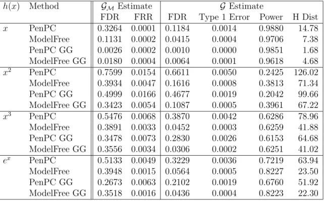
Table 2.1: Simulation Results using (2.4) with Effect Size 1
h(x) Method GM Estimate G Estimate
FDR FRR FDR Type 1 Error Power H Dist
x PenPC 0.3264 0.0001 0.1184 0.0014 0.9880 14.78
ModelFree 0.1131 0.0002 0.0415 0.0004 0.9706 7.38 PenPC GG 0.0026 0.0002 0.0010 0.0000 0.9851 1.68 ModelFree GG 0.0180 0.0004 0.0064 0.0001 0.9618 4.68
x2 PenPC 0.7599 0.0154 0.6611 0.0050 0.2425 126.02
ModelFree 0.3934 0.0047 0.1616 0.0008 0.3813 71.34 PenPC GG 0.4999 0.0166 0.4677 0.0019 0.2042 99.66 ModelFree GG 0.3423 0.0054 0.1087 0.0005 0.3961 67.22
x3 PenPC 0.5476 0.0068 0.3870 0.0042 0.6286 78.96
ModelFree 0.3891 0.0033 0.0452 0.0003 0.6259 41.88 PenPC GG 0.3478 0.0073 0.2830 0.0026 0.6153 64.68 ModelFree GG 0.3556 0.0034 0.0306 0.0002 0.6251 41.02
ex PenPC 0.5133 0.0049 0.3229 0.0036 0.7219 63.94
ModelFree 0.3948 0.0015 0.0564 0.0005 0.8227 23.50 PenPC GG 0.2673 0.0063 0.2102 0.0019 0.6760 51.92 ModelFree GG 0.3518 0.0016 0.0436 0.0004 0.8223 22.30
FDR = False Discovery Rate; FRR = False Recovery Rate; H Dist = Hamming’s Distance.
GG = Indicates the use of the Gaussian Graphical Extended BIC.
Note: Step 1 FDR is calculated against the moral graph and Final FDR is calculated against the true graph.
Once the graph structure is generated, the underlying data structure is assumed to be one of two linear structural equation models:
X = B|h(X) +e. (2.4)
X = h(B|X+e). (2.5)
where, e ∼ N(0, σ2In×n). Without loss of generality, let B be an upper triangular
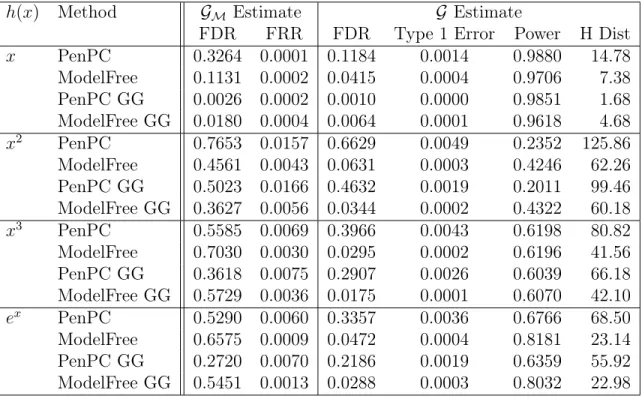
Table 2.2: Simulation Results using (2.5) with Effect Size 1
h(x) Method GM Estimate G Estimate
FDR FRR FDR Type 1 Error Power H Dist
x PenPC 0.3264 0.0001 0.1184 0.0014 0.9880 14.78
ModelFree 0.1131 0.0002 0.0415 0.0004 0.9706 7.38 PenPC GG 0.0026 0.0002 0.0010 0.0000 0.9851 1.68 ModelFree GG 0.0180 0.0004 0.0064 0.0001 0.9618 4.68
x2 PenPC 0.7653 0.0157 0.6629 0.0049 0.2352 125.86
ModelFree 0.4561 0.0043 0.0631 0.0003 0.4246 62.26 PenPC GG 0.5023 0.0166 0.4632 0.0019 0.2011 99.46 ModelFree GG 0.3627 0.0056 0.0344 0.0002 0.4322 60.18
x3 PenPC 0.5585 0.0069 0.3966 0.0043 0.6198 80.82
ModelFree 0.7030 0.0030 0.0295 0.0002 0.6196 41.56 PenPC GG 0.3618 0.0075 0.2907 0.0026 0.6039 66.18 ModelFree GG 0.5729 0.0036 0.0175 0.0001 0.6070 42.10
ex PenPC 0.5290 0.0060 0.3357 0.0036 0.6766 68.50
ModelFree 0.6575 0.0009 0.0472 0.0004 0.8181 23.14 PenPC GG 0.2720 0.0070 0.2186 0.0019 0.6359 55.92 ModelFree GG 0.5451 0.0013 0.0288 0.0003 0.8032 22.98
FDR = False Discovery Rate; FRR = False Recovery Rate; H Dist = Hamming’s Distance
GG = Indicates the use of the Gaussian Graphical Extended BIC, rather than regular BIC.
Note that Step 1 FDR is calculated against the moral graph and Final FDR is calculated against the true graph.
Results for the simulation with 100 iterations and conditional independence testing threshold α = 0.01 can be found in Table 2.1 through Table 2.4. Transformation
h(x) = x2 is a particular challenging case since it is not a monotone transformation. We included it to show that Model Free still performs adequately in this case, with substantial improvements in comparison to PenPC. Hamming’s Distance show a 30%
to 60% improvement when using Model Free overPenPC. Overall, if tuning parameters
are selected by Gaussian Graphical Extended BIC [Foygel and Drton (2010)], both
PenPC and Model Free performed better than their counterparts if we consider false
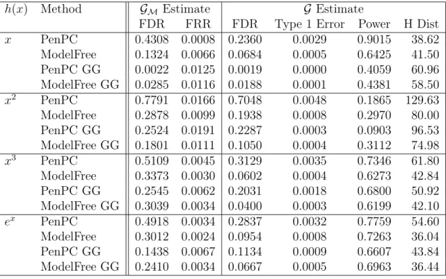
Table 2.3: Simulation Results using (2.4) and Effect Size 0.5
h(x) Method GM Estimate G Estimate
FDR FRR FDR Type 1 Error Power H Dist
x PenPC 0.4308 0.0008 0.2360 0.0029 0.9015 38.62
ModelFree 0.1324 0.0066 0.0684 0.0005 0.6425 41.50 PenPC GG 0.0022 0.0125 0.0019 0.0000 0.4059 60.96 ModelFree GG 0.0285 0.0116 0.0188 0.0001 0.4381 58.50
x2 PenPC 0.7791 0.0166 0.7048 0.0048 0.1865 129.63
ModelFree 0.2878 0.0099 0.1938 0.0008 0.2970 80.00 PenPC GG 0.2524 0.0191 0.2287 0.0003 0.0903 96.53 ModelFree GG 0.1801 0.0111 0.1050 0.0004 0.3112 74.98
x3 PenPC 0.5109 0.0045 0.3129 0.0035 0.7346 61.80
ModelFree 0.3373 0.0030 0.0602 0.0004 0.6273 42.84 PenPC GG 0.2545 0.0062 0.2031 0.0018 0.6800 50.92 ModelFree GG 0.3039 0.0034 0.0400 0.0003 0.6199 42.10
ex PenPC 0.4918 0.0034 0.2837 0.0032 0.7759 54.60
ModelFree 0.3012 0.0024 0.0954 0.0008 0.7263 36.04 PenPC GG 0.1438 0.0067 0.1134 0.0009 0.6607 43.84 ModelFree GG 0.2410 0.0034 0.0667 0.0005 0.6963 36.44
FDR = False Discovery Rate; FRR = False Recovery Rate; H Dist = Hamming’s Distance
GG = Indicates the use of the Gaussian Graphical Extended BIC, rather than regular BIC.
Note that Step 1 FDR is calculated against the moral graph and Final FDR is calculated against the true graph.
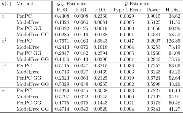
underlying data structure does not substantially effect the performance of Model-Free. While Model Free performs better than PenPC in all cases in Tables 2.1 and 2.2,
we find that Model Free’s primary drawback is a large performance drop with low effect sizes as can be seen in Tables 2.3and 2.4. While for non-linear cases, Model Free still
Table 2.4: Simulation Results using (2.5) and Effect Size 0.5
h(x) Method GM Estimate G Estimate
FDR FRR FDR Type 1 Error Power H Dist
x PenPC 0.4308 0.0008 0.2360 0.0029 0.9015 38.62
ModelFree 0.1324 0.0066 0.0684 0.0005 0.6425 41.50 PenPC GG 0.0022 0.0125 0.0019 0.0000 0.4059 60.96 ModelFree GG 0.0285 0.0116 0.0188 0.0001 0.4381 58.50
x2 PenPC 0.7671 0.0163 0.6843 0.0047 0.2007 126.85
ModelFree 0.2413 0.0076 0.1018 0.0004 0.3253 73.19 PenPC GG 0.2847 0.0182 0.2594 0.0005 0.1260 94.08 ModelFree GG 0.1450 0.0113 0.0396 0.0001 0.2943 73.76
x3 PenPC 0.5115 0.0047 0.3215 0.0036 0.7252 63.66
ModelFree 0.6713 0.0027 0.0469 0.0003 0.6243 42.20 PenPC GG 0.2623 0.0063 0.2125 0.0019 0.6721 52.64 ModelFree GG 0.5029 0.0038 0.0265 0.0002 0.5998 43.26
ex PenPC 0.4929 0.0045 0.3038 0.0033 0.7227 61.14
ModelFree 0.5797 0.0022 0.0745 0.0006 0.7192 34.91 PenPC GG 0.1775 0.0075 0.1443 0.0011 0.6178 50.48 ModelFree GG 0.4714 0.0046 0.0520 0.0004 0.6341 41.27
FDR = False Discovery Rate; FRR = False Recovery Rate; H Dist = Hamming’s Distance
GG = Indicates the use of the Gaussian Graphical Extended BIC, rather than regular BIC.
Note that Step 1 FDR is calculated against the moral graph and Final FDR is calculated against the true graph.
2.5 Application to TCGA Data
2.5.1 Data Source
of 130 gene groups were found, ranging from membership numbers of 1 gene to 2,208 genes. We chose to run the analysis on three clinically interesting groups consisting of p= 64to148 genes with a single random sample ofn= 135patients and cross-validate against the remaining n = 416 patients. The selected gene groups belonged to path-ways: (1) T-Cell Receptor Signaling Pathway (TCR), (2) B-Cell Receptor Signaling Pathway (BCR), and (3) Angiogenesis Signaling Pathway (Angiogenesis).
2.5.2 Analysis Results
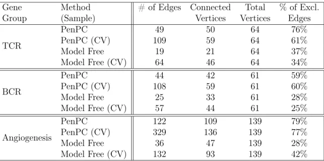
Table 2.5: Results for TCGA Breast Cancer Data
Gene Method # of Edges Connected Total % of Excl.
Group (Sample) Vertices Vertices Edges
TCR
PenPC 49 50 64 76%
PenPC (CV) 109 59 64 61%
Model Free 19 21 64 37%
Model Free (CV) 64 46 64 34%
BCR
PenPC 44 42 61 59%
PenPC (CV) 108 59 61 60%
Model Free 25 33 61 28%
Model Free (CV) 57 44 61 25%
Angiogenesis
PenPC 122 109 139 79%
PenPC (CV) 329 136 139 77%
Model Free 36 47 139 28%
Model Free (CV) 132 93 139 42%
Figure 2.1: Estimated Graphs for TCGA Breast Cancer Data. (a) TCR PIK3CD LCK PIK3R3 BCL10 VAV3 PTPN22 PTPRC UBE2D1 PTEN TRAF6 PTPRJ INPPL1 PAK1 CD4 ERBB3 ZMYM2 EVL IGHV2−70 CSK IGF1R PLCG2 INPP5K PIK3R6 PIK3R5 MALT1 CDC34 PIK3R2 VASP ZAP70 PDK1 CD28 CTLA4 ICOS INPP5D PI3 KB−1027C11.4.1 BCR INPP5J TRAT1 NCK1 PIK3CB PIK3CA HES1 TEC NFKB1 FYB PIK3R1 SKP1 UBE2D2 ITK C2 VEGFA TAB2 PIK3CG CUL1 LYN KB−1208A12.3.1 KB−1460A1.5.1 KB−1562D12.1.1 KB−431C1.4.1 KB−1732A1.1.1 KB−1507C5.2.1 SYK VAV2
● Nodes Connected by Original Sample Estimate Edges found by Both Samples
Edges only found by Cross Validation Sample Edges only found by Original Sample
(b) BCR BCL10 BLNK STIM1 CATSPER1 GAL CACNA1C PTPN6 CS ATP2B1 ORAI1 CATSPERB IGHV3−11 IGHV3−13 IGHV3−21 IGHV4−31 IGHV3−72 RASGRP1 PDPK1 CD19 COIL CD79B MALT1 GRP VAV1 CD22 CATSPERG CD79A TRPM4 RASGRP3 IGKV1−9 IGKV3−11 IGKV1−12 IGKV1−16 IGKV1−17 IGKV6−21 IGKV2D−29 IGKV1D−16 IGKV1D−13 IGKV1D−12 IGKV3D−11 PDK1 IGLV3−21 IGLV2−11 IGLV3−10 IGLV3−9 BCR LARGE MB TRPC1 TEC LARS HLA−C HLA−B FYN CACNA2D1 BLK LYN CA2 SYK SET BTK
● Nodes Connected by Original Sample Estimate Edges found by Both Samples
Edges only found by Cross Validation Sample Edges only found by Original Sample (c) Angiogenesis DVL1 PRKCZ PIK3CD CASP9 EPHB2 PIK3R3 JUN JAK1 F3 WNT2B RHOC NRAS NOTCH2 SH2D2A PLA2G4A PIK3C2B MAPKAPK2 AKT3 PRKCQ MAPK8 TCF7L2 HRAS PIK3C2A ARHGAP1 LPXN BAD PAK1 PDGFD CRYAB ETS1 WNT5B WNT10B FRS2 PTPRB PXN EFNB2 F7 ANG PRKD1 SOS2 PRKCH HIF1A FOS JAG2 DLL4 PLA2G4B MAP2K1 AXIN1 PRKCB TGFB1I1 PLCG2 CRK PLD2 DVL2 MAP2K4 GRAP GRB7 STAT3 FZD2 PRKCA SPHK1 BIRC5 PIK3C3 SHC2 APC2 MAP2K2 PIK3R2 AKT2 PRKD2 PLA2G4C SPHK2 RHOB PRKD3 PRKCE DOK1 NCK2 GRB14 STAT1 FZD5 WNT10A JAG1 SRC PLCG1 CRKL PDGFB PRR5 ARHGAP8 WNT7B RAF1 CTNNB1 RHOA MAPKAPK3 PRKCD WNT5A EPHA3 GSK3B TF EPHB1 PIK3CB PRKCI PLD1 DVL3 EPHB3 PAK2 RBPJ PDGFRA KDR PDGFC MAP3K1 F2R RASA1 APC TCF7 FGF1 PDGFRB DOK3 NOTCH4 MAPK14 FRS3 VEGFA DLL1 PDGFA HSPB1 FZD1 PIK3CG WNT2 BRAF NOS3 ANGPT2 DOK2 FZD3 FGFR1 ANGPT1 PTK2 TEK NOTCH1 ARAF EFNB1 PAK3
● Nodes Connected by Original Sample Estimate Edges found by Both Samples
Table 2.6: Mean Results for Mardia’s Test of Multivariate Normality for Residuals of Exclusive Pairs
Percentile Skew Stat Skew P Kurt. Stat Kurt. P Max Mah. Dis
PenPC 25% 0.226 0.260 9.134 0.099 15.176
50% 0.620 5.91e-03 10.412 4.59e-04 20.525
75% 1.241 8.29e-06 12.510 6.40e-11 30.381
Model 25% 0.473 0.031 9.655 0.016 17.582
Free 50% 1.071 7.628e-05 10.682 1.09e-04 25.164
75% 1.979 6.746e-09 13.233 6.505e-14 37.294
Table 2.7: Similarity and Differences between Estimates from Original and Cross-Validated Sample
Method # Edges in Overlapping P-Value Pos Attr to Attr to Neg Attr to Attr to
Original Edges Discrep Sample Sample Discrep Sample Sample
Sample Total Space Size Total Space Size
TCR PenPC 49 27 4.41e-23 22 18% 77% 82 20% 2%
Model Free 19 10 3.75e-11 9 44% 44% 54 30% 31%
BCR PenPC 44 22 8.47e-16 22 23% 77% 86 28% 2%
Model Free 25 13 2.44e-14 12 42% 42% 44 55% 14%
Angio PenPC 122 64 8.15e-61 58 3% 83% 265 16% 0%
Model Free 36 22 2.12e-32 14 14% 43% 110 39% 16%
Neg Discrep refers to edges not found in the original sample but found in the cross-validation sample.
Pos Discrep refers to edges found in the original sample but not found in the cross-validation sample.
Both PenPC and our Model Free approach were applied to the three different
gene sets using both sets of samples (termed: original and cross-validation). The tuning parameters were selected by Gaussian Graphical extended BIC. Basic summary of results can be found inTable 2.5. Similar to our simulation results, we see thatPenPC
finds more edges than Model Free and accordingly has a larger set of connected vertices. While 25-40% of the edges identified by Model Free are not found by PenPC, around
60-80% of the edges identified byPenPC are not found by Model Free approach. These
trends are consistent between samples. With a much larger sample size, we expect an increase in power and true discovery rate, which agrees with the increased number of edges found in the cross-validation sample for all gene groups across both methods.
Figure 2.1 gives a visualization of the estimated graphs for each gene group as well as the agreement between the original and cross-validation sample. We found the amount of overlap to be statistically significant for all three gene groups across both methods (Table 2.7) against the null that the graphs estimated are independent. To compare the discrepancies between the two sample estimates, we looked at positive discrepan-cies (when the original sample found an edge that was not found in the cross-validation sample) and negative discrepancies (when the original sample did not find an edge that was found in the cross-validation sample). Within these categories, we split the dis-crepancies that can be attributed to sample space and sample size. Disdis-crepancies which occurred when all other results were in agreement were attributed to the difference in “sample size×method interaction” (for example, PenPC found an edge in the original
sample but Model Free did not find it in either sample and PenPC did not find it in the cross-validation sample). Discrepancies which occurred between the original sam-ple and the cross-validation samsam-ple for both methods were attributed to the difference sample space (aka. what was feasible to find within that sample).
can be attributed to either sample size× method interaction or sample space. Sample
size × method interaction is more often the reason for PenPC while two reasons split
more evenly for Model Free method. This indicates that the Model Free method is more volatile across different samples. It also implies that the high false discovery rate of PenPC can be mitigated with sample size. For negative discrepancies, PenPC can attribute less than 30% to sample space, with nearly none attributed to sample size
× method interaction. Model Free attributes over 60% for either reasons and again is
similarly split.
The discrepancies between the two methods can largely be attributed to differences in their model assumptions, namely linearity and multivariate normality. Most PenPC exclusive edges have relatively smaller effect sizes (left panel of Figure F1a), which suggest that PenPC has higher power for smaller effect sizes when linearity assumption is correct. In contrast, Model Free-exclusive edges have more uniform distribution of effect sizes (right panel of Figure F1a), suggesting that PenPC miss those edges because of non-linear relationships rather than effect sizes. We see that this trend is even more pronounced in the cross-validation sample based on Figure F1b. This is congruent with our cross-validation comparison.
For multivariate normality, we looked at whether the residuals of each pair followed bivariate normal distribution given the other variables that had been selected by mGAP. This provides us a proxy for whether the original data followed a multivariate normal distribution. To test for bivariate normality, we used Mardia’s Tests for multivariate normality which tests for deviation of skew and kurtosis, as well as observations with large Mahalanobis distance from the expected distribution [Mardia (1970)]. Full results can be seen in Table 2.6. As expected, on average PenPC-exclusive pairs have smaller
in sample size.
2.6 Discussion
The use of -omic data to guide disease prognosis, prevention, and treatment is becoming a popular approach of precision medicine. The complexity and sheer number of variables within these data sets have set some new statistical challenges. Low false discovery rate is especially important to obtain meaningful results with a large number of variables. In comparison to PenPC, we have shown that Model Free obtains much
lower false discovery rates at a relatively small cost to power when the relation among variables is non-linear. As shown in our real data analysis, Model Free was able to better capture associations that do not satisfy multivariate Gaussian assumption and/or have non-linear relations. Further, Model Free’s lower false discovery rate is reflected in the increased parsimony of the selected models lending to easier interpretability.
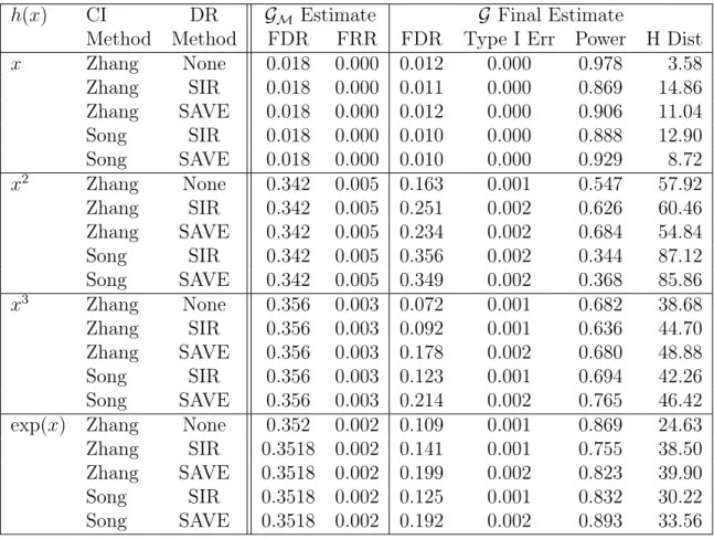
For application in denser graphical models, we may insert a dimension reduction step between model free variable selection and conditional independence testing. This would be particularly useful if the selected Markov Blanket is too large to be handled effectively with KCI-test. We have explored the use of dimension reduction with sliced inverse regression (SIR) [Li (1991)] and sliced average variance estimation (SAVE) [Cook (2000)]. InTable 2.8, we compare the results obtained with or without dimension
reduction to1-dimension, regardless of whether a suitable1-dimension central subspace has been found. In addition to KCI-test, we also include a conditional independence test by [Song et al. (2009)] which requires that the condition set has a dimension of one.
Table 2.8: Dimension Reduction for Model-Free GG Simulation Results using (2.4)
h(x) CI DR GM Estimate G Final Estimate
Method Method FDR FRR FDR Type I Err Power H Dist
x Zhang None 0.018 0.000 0.012 0.000 0.978 3.58
Zhang SIR 0.018 0.000 0.011 0.000 0.869 14.86
Zhang SAVE 0.018 0.000 0.012 0.000 0.906 11.04
Song SIR 0.018 0.000 0.010 0.000 0.888 12.90
Song SAVE 0.018 0.000 0.010 0.000 0.929 8.72
x2 Zhang None 0.342 0.005 0.163 0.001 0.547 57.92
Zhang SIR 0.342 0.005 0.251 0.002 0.626 60.46
Zhang SAVE 0.342 0.005 0.234 0.002 0.684 54.84
Song SIR 0.342 0.005 0.356 0.002 0.344 87.12
Song SAVE 0.342 0.005 0.349 0.002 0.368 85.86
x3 Zhang None 0.356 0.003 0.072 0.001 0.682 38.68
Zhang SIR 0.356 0.003 0.092 0.001 0.636 44.70
Zhang SAVE 0.356 0.003 0.178 0.002 0.680 48.88
Song SIR 0.356 0.003 0.123 0.001 0.694 42.26
Song SAVE 0.356 0.003 0.214 0.002 0.765 46.42
exp(x) Zhang None 0.352 0.002 0.109 0.001 0.869 24.63 Zhang SIR 0.3518 0.002 0.141 0.001 0.755 38.50 Zhang SAVE 0.3518 0.002 0.199 0.002 0.823 39.90
Song SIR 0.3518 0.002 0.125 0.001 0.832 30.22
Song SAVE 0.3518 0.002 0.192 0.002 0.893 33.56
CI Method = Conditional Independence test used for Step 2 DR Method = Dimension Reduction method
FDR = False Discovery Rate; FRR = False Recovery Rate H Dist = Hamming’s Distance
dimension reduction method and conditional independence testing method does not make much difference outside of the quadratic case. SAVE performs better than SIR with the quadratic transformation, which is known from earlier studies [Cook (2000)]. Overall, KCI-test has better performance than [Song et al. (2009)]’s method. Although current results fail to show the advantage of this dimension reduction step, it remains an opportunity for future research.
In this dissertation, we focused on the difference between PenPC and our
other. PenPC can identify weaker effects when multivariate Gaussian and linearity
CHAPTER 3: GRAPHICAL MODEL FOR SCRNA-SEQ DATA
Recall that we denote a DAG skeleton byG = (V,E), whereV ={Y1, ..., Yp}is the
the vertex set, and E is the edge set. A moral graph GM = (V,EM) can be derived from a skeleton G by connecting the co-parents in all the v-structures in G. The data
consists of total read count (TReC) from p genes across n single cells. Similar to the work in the previous chapter, we aim to estimate a DAG skeleton for these p genes in two steps. First construct a moral graph by neighborhood selection. Next remove false edges in the moral graph by a modified PC-algorithm. The specific approaches in both steps are designed to analyze single cell RNA-seq data, which are discrete counts with inflation of zeros.
3.1 Overall Algorithm
give the details of each step in the following sections. Denote the pgenes by Y ={Y1, ..., Yp}. Recall that
• AG,i,j = adj(G, Yi)
Sadj
(G, Yj)\{Yi, Yj}, i.e., the Markov Blanket of Yi and Yj.
Recall that adj(G, Yj)denotes the neighbors of Yj in graph G.
• BG,i,j =adj(G, Yi)Tadj(G, Yj)\{Yi, Yj}, which include all potential common
chil-dren of Yi and Yj.
• CG,i,j = AG,i,j
T
(BG,i,j
S
ConG(BG,i,j)), where ConG(BG,i,j) denotes the vertices
that are connected to BG,i,j. CG,i,j includes any possible common descendants of
Yi and Yj within the Markov Blanket ofYi and Yj.
• Πi,j = {AG,i,j\CG˜ ,i,j,CG˜ ,i,j ⊆ CG,i,j}. At least one of the set in Πi,j includes all
common parents of Yi and Yj, but excludes any common descendants. In other
words, if there is any d-separation set of Yi and Yj, it will be included in Πi,j.
Algorithm 3:Moral Graph Estimation
Data: Y
Result: GM= (V,E)
forj= 1 top do
Let y=Yk and X =Y−k.
Select variables amongX associated withy by jointly penalized zero-inflated
negative binomial regression, denoted by E.
For anyj such thatYj ∈ E, create edgesEk,j and Ej,k. Ek,j ≡Ej,k for the
Algorithm 4:Modified-PC Algorithm
Data: GM= (V,E), X
Result: G
foreach(Ei,j)∈Edo
if Xi⊥Xj then; /* Likelihood Ratio Test */
RemoveEi,j and Ej,i.
l=−1repeat
l=l+ 1
˜
G=G, foreach(i, j);|CG˜,i,j| ≥l do
foreach[Γ; Γ⊆CG˜,i,j,|Γ|=l]do
κ=AG˜,i,j\Γif Xi⊥Xj|Xκ then; /* Likelihood Ratio Test */
Remove Ei,j andEj,i.
Exit while loop and move to nextEi,j in for each loop.
untilmaxi,j|CG˜,i,j|< l;
We refer to our algorithm for DAG skeleton estimation as scZINB, which stands for single cell and Zero Inflated Negative Binomial distribution.
3.1.1 Step 1: Neighborhood selection
We apply our neighborhood selection method for each variable (i.e., a node in the graph) separately. To select the neighborhood of the j-th variable, we model the ob-served count data of the j-th variable by ZINB distribution, and use log-transformed data of all the other variables as covariates. Since our neighborhood selection method is a general variable selection method and it can be applied to other settings, we use more generic notations in the following discussions. Let the observations of the (count) response variable be y = (y1, ..., yn)T and the (continuous) covariate data be